11justwhatissprawl.pdf

Just

What

is

Sprawl,

Anyway?

Urban

sprawlisa hot-buttonissueintheU.S.

Though

thetermiswidelyusedtodescribe thedistastefor contemporary

American

suburban

and

urbandevelopment, aselect

few

group ofresearchers, academics

and

practitionershaveledtheresponsetothe

argument

against sprawl. Thispaperseekstocharacterizesprawl

from

the perspectiveof landscapearchitecture whilefocusing onquantitative

measurements

and

definitions

ofsprawl.

At

itscoreitexaminestheissueofthe evolutionof urban

form

throughtime,

and

offersoptionsfor addressing the debates over the negative orpositiveramificationsofsprawl.

George

R.

Hess, Salinda

S. Daley,

Becky

K.

Dennison,

Robert

P.

McGuinn,

Vanesa

Z.

Morin,

Wade

G. Shelton,

Sharon

R.

Lubkin,

Kevin

M.

Potter,

Rick

E.

Savage,

Chris

M.

Snow

and Beth

M. Wrege

"In thenext threeor four yearsAmericanswillhavea

chancetodecidehowdecentaplacethiscoimtiywillbeto

livein.andforgenerationstocome. .Alreadyhugepatches

of once greencountrysidehavebeenturnedintovast, smog-filled deserts thatareneithercity,suburb,norcountiy.and

eachday

—

atarateofsome3.000acresaday

—

more

countiysideisbeing bulldozedunder Youcan'tstop

progress, theysay.yetmuchmore ofthiskindofprogress

and weshallhavetheparadox ofprosperityloweringour

standard ofliving. ...Theproblemisthepatternofgrowth

—

OK ratherthelackofone."_{(Whyte 1958)}

Introduction

Sprawl

isa hot topic in

America.

Articles about sprawl

have appeared

in

many

magazines

and

newspapers, including Time,

US

News

and

World

Report,

The

New

Yorker, Atlantic Monthly, Sierra.

The

New

York Times,

and

USA

ro<;/m'(Katzand Bradley 1999:

Goldberger

2000;

Moberg

2000:

Thompson

2000;Tolson 2000: El

Nasser

and

Overberg

2001; Firestone

2001). Search for"urban sprawl"

on

the

World

Wide

Web

and

you

willbe inundated witha

combination

of

research,reports,reviews,

and

rants. Inthe

academic

literatureindexed

by

the

Institule

for

Scientific Information's

Science

Citation

Database,

the

number

of

titles

includingthe

word

"sprawl"

had

increased

more

than exponentially.

Indeed, sprawl has

become

theterm people usetodescribealmost anything they

do

notlike

about

American

cities,

from

traffic

jams

on

endless

commercial

stripstocookie cutter

communities on

former farmland.

Negative

effectsattributedtosprawl include

economic and

racial segregation,crime, poverty,loss

of

community,

increased infrastructurecosts,

deterioratingairand waterquality, loss

of

farmland

and

open

space, increasedtraffic

congestion,

and

a generaldegradation inthe qualityof

human

life.

At

the

same

time, a

few

voices

have been

questioningtheconventional

wisdom

thatsprawl

is

bad and "Smart

Growth"

policiesare the cure.

Among

those voices are Peter

Gordon

and

Harry Richardson(1997a).professorsin

Universityof SouthernCalifornia's

School

of

Urban

Planning

and Development,

who

contend

George

R.

Hess

is

an

Assistant Professor in

North

CarolinaStale University's

(NCSU)

Forestiy Department. Tlie co-authors

were

allparticipants in his course.

Measuring

Suburban

Sprawl,

which

was

taughtduringtheSpring

200

J semester This

paper

is

a

product

of

that course.

Salinda

S.

Daley

is

a masters

student in

NCSU's

Zoology

Department.

Becky

K.

Dennison, Robert

P.

McGuinn,

Vanessa

Z.

Morin,

and

Wade

G

Shelton

are masters students in the

Duke

University Nicholas

School of

the Environment.

Sharon

R.

Lubkin

is

an

Assistant Professor

of Biomathematics

at

NCSU.

Kevitt

M.

Potter

and

Rick

E.

Savage

are masters .students in

NCSU's

Forestiy Department.

Chris

M.

Snow

is

a

continuing

education

student

in

NCSU's

Department

of

Parks, Recreation

and

Tourism

Management.

Beth

M.

Wrege

is

a

mastersstudentin

NCSU's

Department

of

Parks,

Recreation

and

Tourism

that

compact

development

isnot a curefor

traffic congestion. Staley(1999) arguedthat

urban

growth

boundaries

do

not reducetraffic

congestion,that

farmland

isnotimperiledb\ urban growth,

and

thatspraw1. itself, isnot bad.

Yetdespite allthe purportedeffects

and

proposed

solutions,a

number

of

researchers noted thatthe

term

"sprawl"

was

rarely quantifieduntil recently(e.g.. Burchelletal.

1998:

Downs

1998; Galsteretal. 2000:

Myers

and

Kitsuse 1999:

Malpezzi

1999).

There

isalso apaucity

of

correlativeanalysis

between

measures of

sprawl

and measures of

social,

economic, and

environmentalquality

—

inpart

because sprawl itselfhas not

been

welldefined

(Downs

1998: Galsteretal 2000).

One

of

thedifficulties inunderstanding

sprawl isthatdifferentobservers

have

definedit

bya

combination of

itscauses(e.g..

zoning

and

poorplanning), characteristics(e.g.. low-density development),

and

effects(e.g.. traffic

congestion

and

airpollution). Galsteret al.

(2000) notedthat sprawl hasbeen defined asan aesthetic

judgement:

as the cause

of

an

externality(e.g..high

automobile dependence,

job-housingspatialmismatch):asthe

consequence of

some

independentvariable (e.g.. zoning): as a

development

pattern(e.g..

low

density, leapfrogging):asa process

of

development

throughtime:

and

by example

(e.g..

w

ith reference to aparticularcity such as Atlanta or

Los

Angeles).

Objectives

Ew

ing(1994).

Malpezzi

(1999).

and

Galster

etal.(2000)

argued

convincinglythatseparating the causes, characteristics,

and

effects of spraw1

isessential toreaching

consensus on what

sprawl is.

We

agree

and

choseto focus our

efforts

on

the spatial characteristicsofsprawl.

Our

primary objective

was

to identify'

and

quantifycharacteristics

of

sprawl

on

the landscape.

What

does

sprawl looklike

on

the

ground?

What

spatial characteristicsshould

one

lookfor todeclare acitysprawled or sprawling?

in thispaper,

we

Characterize sprawl

from

a landscape perspective:

• _Presentquantitativeindices for

some

of

the characteristics

of

sprawl

on

the landscape;

•

Use

_{these indices to}

_compare

_sprawl

among

the U.S.

Census-defined

urbanized areasinthemid-Atlantic United States:

and

•

Measure

_{the correlation}

among

our

indices

and

a

few

purported effects

of

sprawl.

Landscape

Characteristics

of

Sprawl

The word

sprawl hasbeen usedtodescribe

theurban

environment

since the

mid

20'*'_centur\'

(Table 1).

The

Oxford

English Diclionaiy (2001 )

defines itas"the stragglingexpansionof an indeterminateurbanorindustrialenvironmentinto

an adjoiningcountryside: the area

of

this

ad\ancement."

Spraw

1 hasbeen usedasan

adjecti\e describingthe patternof acity"sgrowth,

averbdescribing theprocessofthatgrowth,

and

asa

noun

describinganurban landform.

Although

thefirst use

we

found

was

by

Buttenheim

&

Comick

(1938), the

term

became

relati\ely

commonplace

inthe 1940"s

and

1950"s,

coincident with

two

fundamental

life

changes

in the

United

States

—

an increase in private

automobile

use

and

the

expansion of

the

interstate

highway

system.

While

some

people

were

defining

and

deridingsprawI duringthe

earl> 1950"s.others

were

advocatingthe decentralization

of

American

cities as adefense againstthepossibilityof nuclear

war (Monson

and

Monson

1950. 1

95

1:

Wigton

1953).

However,

these advocates

of

city

decentralizationfavored well-planned,

concentrated

nodes

and were

very

much

against thepoorly

planned

sprawl ofcentralcities

(Monson

and

Monson

1950).

Early uses

of

theterm sprawl suggestthatit

consumes

excessivespace inan uncontrolled,

disorderly

manner

leadingtoloss

and poor

distribution

of

open

spaces,excessive

demand

fortransportation,

and

social separation.

The

"Thefollyofallowingfurlher unrestrictedexpansion

and

disorderlysprawling ofcitiesintoruralareas,

turninggreenfields

and

forests into dreary-city streets

and making

the countryside inaccessibletothe

poorer inhabitants ofthe interiordistricts, isgaining increasing recognition both inAmerica

and

Europe." _(Bultenheim

di Cornick I93H)

"Among

thechiefproblemsfacing London, accordingtotheCountyPlan, werecorigestion. slums,

inadequate

and

maldistributedopenspaces, indeterminatezoning, a/?

J

sprawl, ijone includesthe

London

region. " (Rodwin 1945)

"TheAssociationposesthe alternativeof'self-containedtowns'versus 'suburbansprawl.'

//accusesthe

latterof twobasicfaults:first, excessive

demand

fortransportation

and

second, lackof open spacefor

recreation

and

also expansion." _{(Blumenfeld 1949)} "

... inthesuburbs that hcivebeen

growing

so rapidlyaroundthegreatcenters the buildingsexist,

ideally, as free-standingstructures inaparklike landscape. Too often thetrees

and

gardens vanish underfurther pressure ofpopulation, yetthesprawling, openindividualistic structure, almostanti-social

in itsdispersed

and

its

random

pattern, remains."

_(Mumford

_{1953: 223)}

"

... theaimlesssprawlofsuburbiaisdestroying a preciousasset (openland). "(Haskell 1958)

"Greatsizehasanother featurethatisn'tquitesobeneficent. With veiy greatpopulationsizecomesveiy

great area(aswellashighdensity): and. withthe increasinguseoftheautomobile,

we

get 'sprawl,'

allof whichleadsto intra-area spatialpatterns characterizedby veiyconsiderable socialseparation. "

(Thompson

1966)

Table I.

Some

earlyusesofthe

word

"sprawl"to describeurban growthpatterns.

essential elementsofthese early definitions

have

remained

relatively

unchanged

throughtime. In

her report. Revisiting Sprawl:

Lessors

From

the Past,

Burgess

(1998:1)defined sprawl as

".

..

expanding

physical

development,

at

decreasingdensities,inmetropolitanregions,

where

thespatial

growth

exceeds

population growth."

Lee and

Tian (1998) suggested that

urban sprawl leadsto inefficient land-use. leapfrogging,

and

low-density

development of

the urban fringe.

The

Sierra

Club

(1998) defined sprawlas"iow-density

development

beyond

the

edge of

service

and

employment,

which

separates

where

people live

from

where

they shop. work, recreate,

and

educate

—

thus requiring carsto

move

between

zones."

Brueckner

(2000) defined urban sprawlas excessivespatial

growth of

cities.

Aftera

comprehensive

literature review

(Hess

2001).

we

noteda

number

of

common

characteristics

among

sprawl definitions(Table 2).

Ewing(1994.

1997).

Malpezzi

(1999).

and

Galsteretal. (2000) provided valuable reviews

of

sprawl definitions.

The

characteristics

associated

most

frequentlywith sprawl

were

low-densitydevelopment,stripdevelopment, scattered

development

away

from

the central city, leapfrogdevelopment,

and

separation

of

land uses. Density is by farthe

most

common

measure, followed by

comparisons

between

the

rateat

which

land isurbanized

and

therate

of

population

growth

(e.g.. land

was

urbanizedat three timestherateof population growth).

Ewing

(1

997)

arguedthat

poor

accessibility

—

difficulty

moving

among

widely separatedland

uses

—

and

a lackoffunctional, public

open

spacesare the primary hallmarks

of

sprawl.

There

seems

to be general

agreement

that sprawl isa matter of degree. For

example,

it is

difficulttosayat

what

density acity

becomes

sprawled,butrelativelyeasy tosaythat

one

city is less

dense

than another

and

therefore

more

sprawlingin thataspect.

Some

researchersconsider time to bea

critical

component

inthe

measurement

of

sprawl

(US

EPA

2000;

Ewing

1994;

Harvey

and Clark 1965).

Harvey and

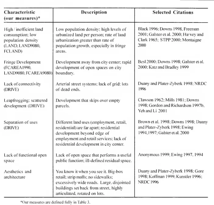
Clark (1965) notedthat

Characteristic

Description

Selected Citations

(our

measures)*

High/inefficientland

Low

populationdensit>: high levelsof Black1996;

Downs

1998,Freeman

consumption; low urbanized landper person;rate ofland 2001;Galsteretal.2000:Ha-vey and population density urbanizationgreaterthanrateof Clark 1965;

STPP2000:

Montaigne

(LAND.LAND9080,

populationgrowth,especiallyinfringe 2000

FCLAND)

areas.

FringeDevelopment Development

away

fi"om citycenter:rapid Besl2000:

Downs

1998; Galsteretal.

(FC

AREA!

990. development of open spaces oncit\ 2000;KatzandBradley 1999

LAND9080, FCAREA9080)

boundary.

Lack ofconnectivity Arterial streetsystems: lackofgrid; lots

Duany

andPlater-Zyberk 1998;

NRDC

(DRIVE) ofdeadends.

19%

Leapfrogging: scattered Developmentthatskipsoverempty Clawson 1962:Mills 1981:

Downs

development

(DRIVE)

parcels. 1998;

Gordon

andRichardson 1997b,

o

YehandLi

2001

CNJ tt:

1

Separationofuses Different landuses(employment,retail.

Brown

etal. 1998;

Downs

1998;

Duany

(DRIVE) residential)arefarapart:residential andPlater-Zyberk1998;

Ewing

CO development beyond edge of

emplo\ment

andretailservices; lackof

1994. 1997; Galsteretal.2000

i

residential developmentincity center.

Lack offunctionalopen Lack of openspacethatperformsauseful

Anonymous

1999;

Ewing

1997, 1994

a.

1

space publicfunction; ill-detlnedresidual space.

o

q:

s

Aesthetics and

You

know

it

when

youseeit. Big-box

Duany

andPlater-Zyberk 1998;Gore

architecture retail:stripmalls;nosidewalks; 1998;Koffman 1999; Kunstler1996:

excessivelywideroads. Large,disjointed

NRDC

1996

buildingssetback from street,highly articulated,rotatedonlots.

*()urmeasuresaredefinedfully inTable3.

Table2. Spatial characteristics of sprmvl

found

inthe literature.

moment

in time,

because

sprawl isa

form

of

quantitativeapproachestodefining sprawl, yet

few

growth.

They

arguedthat it isthe trendin have developed

comprehensive

ways

to

measure

populationdensity,ratherthancurrentpopulation sprawl.

The

Sierra

Club

(1998) rankedU.S.

density,thatdetermines

whether

a cityis Census-detlned urbanizedareasby considering sprawlingornot.

A

city

becoming

lessdensely trendsinpopulationandland areagrowth,traffic populated through timeissaid tobe sprawling. congestion

and open

spacelossindicators.

They

even ifitiscurrently quitedensely populatedin alsoaccountedfor lossof important

w

ildlifehabitat

comparison

toothercities.

and

historical sites. In

USA

Today,El

Nasser

and

Overberg

(2001) rankedall

of

the

US

Census-Approaches

to

Measuring

Sprawl

detlnedMetropolitanStatisticalAreas

by

considering trendsinthe proportionofthe Several authorshavedecried the lack

of

populationintheMetropolitanStatistical

Areas

livinginurbanizedareas.

iviaipezzi(1

999) and

Galsteretai.

(2000)

lia\e

done

tiie

most

cogent\vorl<todate, focusingprimarily

on

measuring

thespatial

characteristics

of

urban landscapes.

Malpezzi

(1999)

examined

several

measures

ofthe spatial

distributionof populationdensity'

among

census

tractsofall U.S. Metropolitan StatisticalAreas.

He

compared

overall density:

maximum

and

minimum

tractdensity:densityofthe

median,

tenth,

and

ninetiethpercentile

population-weighted

tracts: coefficientofvariation

of

the

tract densities:Theil's information

measure:

the

Ginicoefficient:parameters

of

the densities" tit

toa spatialexponential or otherfunction:the

r-square statistics thereof:

and

the average distanceof each person tothe central business district.

He

found

strong correlations

among

the percentile measures,

and

weaker

correlations

among

the othermeasures.

Malpezzi

also

examined

thecorrelation

between

spatial

measures and

commuting

measures,

and found

(with strong correlation)thatdenserareashave shorter

commutes, and

thatareaswithhigh

median

home

prices alsohaveshorter

commutes.

Galsteret al. (2000)

examined

sixdifferent

measures

ofresidential

development:

1

)

Density, the average

number

of

residential unitspersquaremile: 2) Concentration,thedegreeto

which

development

islocatedwithin a relatively

few

square miles

of

the urbanized area:

3)

Compactness,

thedegree to

which

development

has

been

clustered: 4) Centrality,the degreeto

which

development

is located close to the

centralbusinessdistrict:

5) Nuclearity, the extentto

which

an urbanized area ischaracterized

by

a singlecenter

of development: and

6) Proximity

of

land uses, thedegreeto

which

different land usesarecloseto

one

another.

They

applied these

measures

tothirteen large U.S. cities

and

ranked

them

from

least to

most

sprawled accordingto each ofthe

above

six measures.

They

further

summed

all

of

the ranks foracityto provide anoverall

measure

of sprawl foreach city. Galsteretal. (2000)also

proposed

two

other

measures

forfuture

de\elopment:

com

innif}-, thedegreeto

which

landhas

been

developed inan

unbroken

fashion:

and

diversily

_of

luud nses. the degree to

which

differentland usesexistwithinportions

of

the urbanizedarea.

Yeh

and

Li(1998,

2001)

used a geographical

information system(GIS)analysis

of

remotely sensed data to

measure

and monitor

the degree

of

urban sprawl for cities

and towns

inChina.

They

characterized sprawl as scattered

new

development on

isolated tractsseparated

from

otherareas

by

vacant land.

To

quantify the degree

of

scatteringthey calculated

Shannon's

entropy,a statistical

measurement

of

dispersion based

on

therelative

numbers

of an item (the

amount

of

new

development, in thiscase) in

each

of

several

compartments

(concentric rings

around

a city, inthiscase). Cities

and

towns

with higher entropy values

were

characterizedas

more

sprawled

because they exhibited

more

dispersed

development

—

the

new

development

was

spread evenly

among

the

compartments.

Yeh

and

Li also usedentropy to

measure

dispersal

of development

along

major

roads

and

highways.

Although

Yeh

and

Lididnot

do

so.a

seriesof entropy measures through time can be

usedtodeterminechangesinthedegreeto

which

a

city's

development

isdispersed orcompact.

Our

Measures

of

Sprawl

We

defined seven

measures

that relate

directlytoseveral spatial characteristics

of

sprawl (Table 3).

We

restricted ourefforts to

measures

thatcould becalculated using data readilyavailableinastandardized formatfor

cities nationwide.

We

focused ourefforts

on

U.S. Census-defined urbanized areas,

because

theyaredefinedconsistentlythroughoutthe United States.

We

used

1990

United States

Census and

related Federal

Highway

Administration data,

because

theyare the

most

recent dataavailable forurbanized areas in the United States.

Most of

the

measures

reflect

landconsumption,differences

between

land

consumption

in the center

and

fringe

of

the urbanizedarea,

and

changes

in land

consumption

1

Measure

Description

/

Rationale

(Data Source)

Formula

AREA

LAND

Land

Consumption

Area

of urban area(square miles) in 1990. Larger urban areas

consume more

land,

and

areconsidered

more

sprawling.

(US

Census Bureau)

Urbanized

land percapita in 1990. Size

of

urban area/

population(acresper 1.000people).

A

more

sprawlingcit\ uses

more

land per person.

(US

Census Bureau)

UA*

Area

UA

Area(acres)

UA

Population(1.000s

)

i

CO

FCAREA

FCLAND

Population Concentration

Fringe-to-centerarearatioin 1990. Ratio

of

fringe areatoarea

of

cit> center.

Sprawled

citiesare said toha\e

more

de\elopmentavva\

from

theircit} centers.

(US

Census

Bureau) Fringe-to-center landpercapitaratioin 1990. Ratio

of

land

used percapitain the fringetoland used percapita inthe cir\ center.

Sprawled

cities areoften said to

ha\e

much

higher land

consumption

percapita inthe fringethaninthe center.

(US

Census Bureau)

Areaof

UA

Friniie Areaof

UA

Center

FringeArea/Fringe

Pop

Center.Area/Center

Pop

9

1

s!

i

o

2

DRIVE

Separation of

Land

Uses/Accessibility

DaiK

Vehicle

Mileage

perCapitain 1993. This

measure

reflectstheaverage dailymileage per capita relativeto cities

of

the

same

population density.

>

1

means

more

dri\ingthan averageforcities

of

same

density

<1

means

lessdriving than averageforcities

of

same

density

We

usedthis indexasa surrogateformeasuringseveral spatial

characteristicsofsprawl. Separation oflanduse. lackof

connectivit},

and

pooraccessibility are spatial characteristicsof spraw1thatresultinincreaseddri\ing

and

higher\aluesofthis

index.

(US

Federal

Highwav

Administration)

Obser\ed

DaiK

Milease ExpectedDailyMileage (Seetextfordetails)

FCAREA9080

LAND9080

Temporal

Development

Patterns

Ratiooffringe-to-centerarearatioin

1990

to

1980

value. Cities are

more

sprawling

when

the size

of

theirfringeareas increases fasterthan the sizeoftheir centers(i.e.,

FCAREA9080

>

1).

(US

Census Bureau)

Ratioof

urbanizedlandpercapitain

1990

to

1980

value. Cities are sprawling

when

their rate

of

land use percapita is

increasing (i.e..

LAND9080

>

1).

(US

Census Bureau)

FCAREA

(1990)

FCAREA

11980)

LAND

(1990)

LAND

(1980)

*L

A

=

US

Census-defined urbanizedarea

Table3. Ouantitarh-emeasuresofsprawlthat

we

caladated. Forallmeasures, higher valuesindicate

more

sprawl.

The

U.S.

Census Bureau

definesan

urbanized areaas

one

or

more

central places

and

theadjacentdenselysettled urban tVinge that

togethercontaina

minimum

of50.000 persons

(US-DC

1994).

The

definition has

been

used since

1950

topro\idea better separation of urbanandrural territory,population,

and

housmg

inthe vicinity

of

placeswithrelativelylarge populations.

The

definitionhas

changed

somewhat

throughtime,but has

been

relatively

consistent since 1970.

The

urbanfringe

generallyconsistsof contiguousterritory

having

adensity ofleast 1.000 personspersquaremile.

The

urbanfringe alsoincludesoutlyingterritory,

ifitis

connected

tothecoreofthecontiguous area

by

road

and

iswithin 1.5 road milesofthat

core, orwithin fiveroad milesofthecorebut separated

by

waterorotherundevelopable

territory.

Other

territorywithapopulation

density

of fewer

than 1.000people per square

mileisincluded intheurban fringeifiteliminates

an enclave or closesan indentation in the

boundary of

the urbanizedarea.

Our

early analyses

showed

that the size (squaremiles)

and

population

(number of

people)

of

urbanized areas

were

correlated atthe total

(r=0.97). fringe (r=0.99).

and

center (r=0.70)

scales.

Because

we

were

focusing on landscape

characteristics,

we

chose to

work

with area

measures

insteadof population measures. Similarly,

we

used

measures

ofland

consumption

—

the

amount

ofland used per person

—

which

istheinverseof population density.

One

canalso

measure

land used per

housing

unit:however, housingunitdensity

and

populationdensity

were

completelycorrelatedin our studyarea (r=1.0).

Separation

of

landuses andaccessibilityare important

and

related

dimensions

of sprawlthat

aredifficult to ineasuredirectly.

The

term

"accessibility"isusedin thesprawlliteratureto represent the ease of

movement

among

different land uses, especially

home,

work,

and

services (e.g..

Koenig

1980). Accessibilityisinfluenced

by

thedegree to

which

these land usesare separated

on

the landscape. Personal

transportation surveys (e.g..

US-FHA

2001)

are the best

approach

to

measuring

accessibility,

because

the\ provide information about

what

peoplearedoing,

where

theyaregoing,

and

how

they are gettingthere. Unfortunately, theyare costlyto

implement and

availableforonlya limited

number

of

MetropolitanStatisticalAreas.

We

used averagedaily vehiclemilestraveled per person as a surrogate

measure

for degree

of

accessibility

and

separation

of

land uses. Daily vehicle milestraveled perpersonare reported

by

Census-defined

urbanizedarea in theannual U.S.

Department

of Transportation

Highway

Statistics publication.

The

data arebased

on

a

statisticalanalysis

of

trafficcounts usingthe

Highway

Performance Monitoring

System

(Office

of

Highway

Policv Information 2000).

We

used data

from

the 1993

Highway

Statistics

(Officeof

Highway

Information

Management

1994). becausethese

were

the first

developed

using 1

990

urbanized area boundaries.

One

must

becareful

when

comparing

cities

of

differentdensities,because vehiclemiles traveleddecreases with increasingpopulation density(e.g..

Ewing

1997). Therefore,

we

developed

a

"DRIVE"

index thataccounts for populationdensity.

By

fittingacurvetodaily vehicle milestraveledperpersonasa function

of

populationdensitv',

we

were

able to calculate the expecteddailyvehiclemilestraveled

(DVMT)

based on thedensity

of

acity.

Our

index

was

obtainedbycalculating

DRIVR Ob'.erved

DVMT

/person

tixpetlcdDVMT/person. basedonurbanized area density

Because

theindex isnormalized

by

urbanized areadensity,it isonly

comparing

cities

oflikedensity.

We

arguethat higher values

of

thisindexare relatedtorelativelyhigh

automobile

usethat results

from

greater separation

of

land uses

and

pooreraccessibility.

Applying

Our

Measures

of

Sprawl

to the

Mid-Atlantic

Urbanized Areas

We

applied ourseven

measures

(Table3)to

the forty-ninecitiesintheseven mid-Atlantic

states (Delaware.

Maryland.

New

Jersey.

North

Carolina.Pennsylvania,Virginia,

West

Virginia) that (1)

were

considered urbanized areas in both

Highway

Administration data

were

available.

We

ranked the cities accordingtothe degree of sprawl foreach characteristic (Table 4).

We

alsoevaluatedthe linear correlation

among

the seven measures,

and found

that

none of

the

measures were

highly correlated (Table 5).

The

highest

magnitude

of

any

correlation (0.48)

was

between

the fringe-to-centerarea

and

land

consumption

ratios;

most

correlations

were

much

weaker. Thislack

of

strongcorrelationimplies

thateach indexis

measuring

something

different.

Agglomerative

Cluster

and

Principal

Components

Analyses

An

agglomerati\e cluster analysis

was

used

to identify groups

of

cities

w

ithsimilar

characteristics. Clustering isa

mathematical

techniquethat

groups

entities

w

ithsimilar

attributes

by measuring

thedistance

between

them

in multidimensionalspace.

At each

stepin anagglomerativecluster analysis,the

two

entitiesorgroups

of

entitiesthatare

most

similar

to

one

anotherare

grouped

into a singlecluster.

A

number

of approaches

can be taken to

measure

the distance

between

clusters.

We

used

Ward's

Method, which measures

the variance

between

clusters at each step

and

joins the clusterswith the

minimum

variance.

The

clusteranalyses

were performed

using

JMP

(SAS2001).

We

also

performed

aprincipal

components

analysis

on

our measures. Principal

components

anah

sis isanumerical

method

usedto analvze multi\ariatedata

(Legendre

and Legendre

1998).

It isan ordinationtechniquethatis usedto

summarize

trends

and

patterns

among

samples

(urbanizedareas, inourcase). gi\ena

number

of

characteristics for each sample.

The

output ofa principal

components

analysis isascorethat

combines

the characteristicsthatexplain

most of

thevariance

among

samples.

The

principal

components

analysis

was

performed

using

PC-ORD

(MjM

Software

Design

2000).

Both

cluster

and

principal

component

analyses

were performed on Z-transformed

indices, orZ-scores.

A

Z-score isthe

number

of

standardde\ iationsan observation is

from

the

mean

of

the distribution.

We

used Z-scores

instead

of

theraw indexvalues,

because

the index \alues

were of

ver}, differentmagnitudes. Cluster

and

principal

component

analysis are

sensitixetolargedifferencesin

magnitudes

andwill

return spuriousresultsifdata are nottransformed.

We

usedcluster

and

principal

components

analysesto

group

citieswithsimilar

characteristics

of

land

consumption

(LAND),

fringe-to-center land

consumption

ratio

(FCLAND).

and

daily vehiclemilestraveledper person.

We

usedthe

observed

dailyvehicle milestraveledperperson ratherthan our density-adjusted

DRIVE

index,

because

density

was

incorporated intotheanalyses(through

LAND)

and

both

methods

therefore accountfor

differencesin densit\.

According

toourcluster

anaK

sis.

most

of the difference

between

groups ofcities

was

explained

by

overallland

consumption

(LAND),

followed

by

the fringe-to-centerland

consumption

ratios

(FCLAND).

followed

by

dailyvehiclemilestraveledper person. Principal

components

analysis

of

the

same

variables

yieldedsimilarresults(Table4).

The

first principal axiscaptured 57 percentofthe variance inthedata,

and

was

most

closeh associated with land

consumption

(LAND)

and

daily vehiclemilestraveledperperson.

The

second

axiscaptured an additional

24

percent

of

the variance

and

was

most

closelyassociated

w

iththe fringe-to-centerland

consumption

ratio

(FCLAND).

The

larger,oldercitiesall

had

relatively low levels

of

land

consumption and

relatively

low

levels

of

dailydri\ingpercapita.

Among

cities

withlow levelsoflandconsumption,daily driving

percapita

was

relatively low.regardless

of

the

Table4 (right). Sprawlrankings of 49

urbanizedareasintliemid-Atlanticstates

from

most sprawled(I) toleastsprm^'led(49). Thefirst columnliststheurbanized areas

from

mosttoleast

sprawlingasranked bythefirstprincipalaxisof a principalcomponents analysis ofoverallland consumption (LAND),fringe-to-centerland consumptionratio

(FCLAND). and

observeddaily

vehiclemilestrcn-eled. The remaining columns

show

therank of each urbanizedareaforeach ofour sevensprawlindices,

from

themostspra\\iedll)to

LAND

FCAREA

City (principalaxisI)

AREA

LAND

FCAREA

FC

LAND

DRIVE

9080

9080

1. AshevilleNC 23 7 32 31 4 34 30

2.

HickonNC

32 5 24 42 5 23 45

3. Vineland-MillvilleNJ 15 1 48 49 44 48 35

4. Kingsport

VA

20 1 27 43 23 ~n 44

5. Lynchburg

VA

19

->

39 29 20 24 6

6. Bristol

Tn7vA

38 4 44 24 22 37

7. HighPoint

NC

30 14 41 41 13 20 38

8.

BurhngtonNC

39 17 34 38 1 31 24

9.

GastoniaNC

27 13 30 37 11 27 36 c_

C

10.Raleigh

NC

11 23 40 32 J-> 11 10 -1

11.Greensboro

NC

25 32 47 22 -) 25 41

_X

12.Winston-Salem

NC

16 20 42 26 10 41 31

^

13.Danville

VA

42 8 49 19 24 49

C/)

14.Wilmington

NC

29 6 31 27 32 44 39

i

15.GoldsboroNC 40 11 35 15 38 46 46

16.Norfolk-VirginiaBeach

VA

9 43 13 37 "1 48

>

z

17.

Durham

NC

18 30 46 44 16 26 47

18.Charleston

WV

21 21 26 46 12 4 4

$

o

19.AtlanticCity

NJ

17 16 13 40 14 8 29

20.Charlotte

NC

21.Roanoke

VA

8

26

27

31

45

38

23

45

19 17

47 42

18

20

_O

22.Petersburg

VA

19 29 47 36 19 1

m

O

23.

Richmond

VA

7 29 19 34 7 40 9

_o

24.FayettvilleNC 14 24 25 48 39 43 32

m

73

25.Hagerstown

MD

44 T) 21 14 28 36 19

X

26.Huntington-Ashland

WV/KY

24 25 23 33 29 7 8

m

w

(Si

27.Annapolis

MD

37 18 11 5 31 5 11

m

—

t

28.Jacksonville

NC

31 12 16 30 48 49 40

>

29.Parkersburg

WV

48 36 37 39 40 6 7

jO.AIIentownPA

13 42 -n 28 30 35 15

31.Charlottesville

VA

47 39 25 33 14 5

32.Altoona

PA

46 40 28 8 41 21 25

33.Scranton-Wilkes-Barre

PA

9 28 14 20 42 30 T)

34.Harrisburg

PA

12 26 T 16 8 28 34

35.Sharon

PA

43 10 5 3 49 1 1

36.Erie

PA

M

41 36 35 45 9 27

37.Johnstown

PA

45 yi 17 17 43 15 26

38.Baltimore

MD

6 43 12 10 18 18 17

39.Wilmington

DE

10 37 7 36 15 39 43

40. Reading

PA

35 46 18 11 34 33 13

41.StateCollege

PA

49 45 20 1 47 10

-1

42.Trenton

NJ

~n ₄₄

4 4 9 38 23

43.York

PA

36 38 8 9 21 32 14

44.

Monessen

PA

41 15 1 21 46 13 12

45.Washington

DC

4 47 9 18 6 45 37

46.Pittsburgh

PA

5 J.5

-1

12 35 12 28

47.Lancaster

PA

28 35 6 7 27 29 16

48. Philadephia

PA

T ₄₈

10 6 25 17 21

PC

PC

LAND

PCAREA

AREA

LAND

LAND

AREA

9080

9080

DRIVE

AREA

1

LAND

(0.31) 1

FCLAND

0.38 (0.44) 1

FCAREA

0.14 (0.32) 0.48 1

LAND9080

0.03 0.07 0.31 0.13 1

FCAREA9080

(0.2) (0.17) 0.27 0.22 0.43 1

DRIVE

0.02 (0.04) (0.26) (0.12) (0.27) (0.27) 1

PC

1 (0.30) 0.79 (0.60) (0.68) (0.11) (0.30) (0.41)

Table5. Correlations

among

sprawlmeasures. Sprawl measuresare definedin Table3:

PCI

isthescoreofthe firstprincipal components axis: negativenumbers are

shown

inparentheses.

fringe-to-center

consumption

ratio.

No

cities

had

both high levels

of

land

consumption and

ahigh

ratio

of

fringe-to-center land

consumption,

in

essence, both the core

and

fringe ofcitieswith highrates

of

land

consumption were developed

atsimilar densities. Citieswith high land

consuinption levels

were

further differentiated

by

the relative

amounts

of

drivingpercapita.

Many

of

thecitieswith highlevels

of

dailydrivingper capita

have

recentlyexperienced periods

of

high

growth and

economic

prosperity.

Correlates

of

Sprawl:

Porest

Fragmentation

Background

Widespread concern

about environmental degradationasaresult

of

regional

development

patterns

emerged

in the 1960"s

and

1970"s (Burgess 1998).

Land

transformation has been cited as the

major

forcedrivinglosses in biological diversity(e.g..Vitouseketal. 1997). Habitatfragmentation, inparticular,hasbeen

documented

as

having

negativeeffects

on

biodiversity

by

increasing

"edge

effects."

and

isolatinganimal populationsatavariet}'

of

spatial

scales

(Lovejoy

et al. 1986.

Laurance

etal.

1997).

Though

rarely

mentioned

directly,issues relatedtofragmentation, such as loss

of and

limited accessto

open

space, are often cited as negativeeffectsof "leapfrogging"

development

(Downs

1998: Evving 1994. 1997).

Sprawling

development

issaidtoresultinsmall, isolated patches

of

habitat

surrounded by

landin

residential,

commercial,

orindustrialuses. Inthe

mid-Atlanticregion,

concern

abouthabitat fragmentation is

focused

on

forestedhabitat,

largely

because

forestis the

climax

vegetative

community

intheregion.

Methods

We

tested the hvpothesisthatthe degreeof

forest fragmentation in

and around

an urbanized

area is directlv related tothe degree

of

sprawl.

We

usedforestfragmentation

maps

developed

by

Riitters.etal. (2000)

from

Multi-Resolution

Land

Characteristics

(MRLC)

land-cover

maps

derived

from

1

992 Landsat Thematic

Mapper

(TM)

data, at

30 meter by 30 meter

resolution.

Riittersetal. (2000) assigned

one

of

six

fragmentation categoriestoeach forest pixel based

on

the land

cover

inthree fixed-area

windows

surroundingthe pixel (9x9.27x27.

81x81).

Fragmentation

categoriesare: interior,

perforated,undetennined.transitional,edge,and patch.

We

useddata

from

thesmallest scale

(highest resolution)vv

indow

(9x9)forouranalysis.

We

considered allbut the forest interior

category to be

fragmented

and

calculated the proportion

of

allforestpi.xelsthat

were

interior

forest in each urbanized area.

Because

sprawl

is saidto affect habitatnear urbanized areas,

we

also calculated thepercent interior forest ina five-kilometerbuffer

around

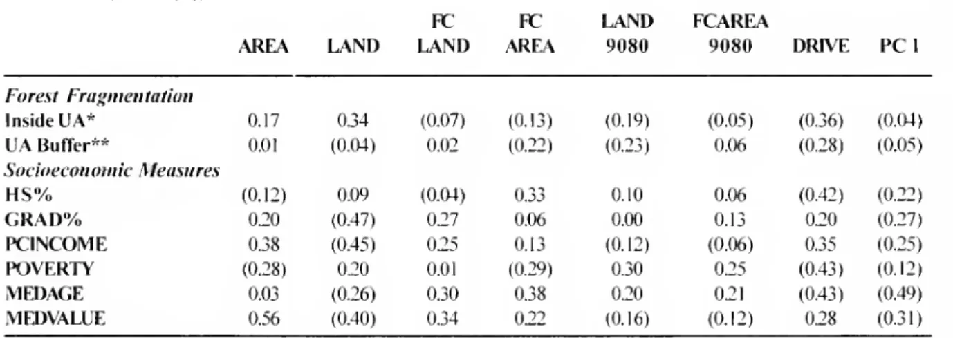
theurbanizedareas.

Findings

Neithertheproportionofinteriorforest

withintheurbanized areanortheproportion in

the fivekilometer region

around

theurbanized area

were

correlated stronglywith

any

of our

measures

of sprawl (Table6).

Socioeconomic

Measures

Background

Because

sprawl has

been

blamed

for a variety

of

social ills,

we

setouttodetermineif

any of

our

measures were

correlated with easily

measured socioeconomic

indicators, hi

Sprawl

City: Race. Politics,

and

Planning

in Atlanta. Bullardetal. (2000) presented

arguments

that

typifythediscussion of

socioeconomic

issues relatedtosprawl. Bullardetal.(2000) theorized

that

government

policy,includinghousing, education,

and

transportationpolicies,

have

subsidizedseparate butunequal

economic

development,

segregated neighborhoods,

and

affectedthespatial layout

of

central cities

and

suburbs.

They

offeran environmentaljustice

framework

with

which

to investigate the social

effects

of

sprawl

on

minority

and low-income

individuals.

Environmental

justice

encompasses

environmental racism

—

discriminationthat

targetspeople

of

color

and

certain

socioeconomic

backgrounds and

excludes

them

from

planningdecisions

—

and

environmental

inequity,

which

deniesethnic

and

low-income

individualsaccessto

employment

centers.

Methods

and

Findings

We

selected a

number

of

socioeconomic

attributesavailable

from 1990

US

Census

data

and

examined

theircorrelationwith our

measures

of sprawl (Table 7).

None

ofthe

attributes

were

correlated stronglywith our

sprawl

measures

(Table6).

We

examined

scatterplots

of

the

moderately

correlated(>0.4) pairs

and found

thatthey

were

dominated by one

or

two

outlyingvalues,

making

any

generalizations suspect.

Although

the

relationship is

weak(r=0.43),

our indexofland useseparation

and

accessibility

(DRIVE)

does appear to increase as the

median

age

of housing

(MEDAGE)

decreases.

The

implicationis that

urbanizedareaswith

new

housing

stock

have

a largerseparation

of

land uses

and

poorer

accessibility,resultingin

more

driving.

Future

Work

Our

sample

size

was

relativelysmall in terms of

performing

cluster

and

principal

components

analyses,

and

New

York

was

an outlier in several respects (e.g.,area,density).

Applying

our

PC

PC

LAND

FCAREA

AREA

LAND

LAND

ARF^

9080

9080

DRIVE

PCI

Forest Fragmentation

Inside

UA*

0.17 0.34 (0.07) (0.13) (0.19) (0.05) (0.36) (0.04)

UA

Buffer** 0.01 (O.W) 0.02 (0.22) (0.23) 0.06 (0.28) (0.05) Socioeconomic

Measures

HS%

(0.12) 0.09 (0.04) 0.33 0.10 0.06 (0.42) (0.22)

GRAD%

020

(0.47)

027

0.06 0.00 0.13

020

(027)

PCINCOME

0.38 (0.45) 025 0.13 (0.12) (0.06) 0.35 (0.25)

POVERTY

(0.28)

020

0.01 (0.29) 0.30

025

(0.43) (0.12)

MEDAGE

0,03 (0.26) 0.30 0.38

020

021 (0.43) (0.49)

MEDVALUE

0.56 (0.40) 0.34 022 (0.16) (0.12)

028

(0.31)

* _IJ.A=

US

Census-defined urbanizedurea

**_Withina5-kilometerbulTeraroundtheurbanizedarea

Table6. Correlations henveen sprawl measiovs

and

measures ofpotentialenvironmental

and

socioeconomiccorrelates. Sprawl measures

and

definitionsareprovidedin Table3:

PC

I isthescoreofthe

firstprincipalcomporients axis:fragmentationvariables are describedinthetext: socioeconomicvariables

are describedin Table ''. _{Negativenumbers}

Iariahle Description /Rationale

EdiicatioiKil Aiuiinineni

HS%

GRAD«c

Percent of people age25 >ears and olderfor

whom

high school orgraduate school is thehighest

levelofeducation. Higher levelsofeducation generallytranslateto higherincome and increased abilit) to satisfS preferencefor low-densit)'housing. Expecthigherlevelof educational attainment tobecorrelatedpositiveK withsprawl.(Bullardetal.2000)

Income

PCINCOME

POVERTY"

Percapitaincomeforpeople age5yearsandolder. Insurveys, upperincomeindividualsexpressed

a desire forlow-densityhousing andthe flexibility tobemobile. Expectsprawlingcities tohavea

higherper-capitaincome. (Bullardetal.2000)

Percentofindividualsage5 yearsandolder

who

fallbelowthe 1989povertyline. Sprawlleavesa decayinginnercity with highratesofpoverty. Expect sprawlingcitiestohave higher povert> levels.

(Bullardetal.2000)

Huusing

MEDAGE

MEDVALUE

Median

age ofhousing stock in 1989. Duringthe 1950s-1970s.the influx oftractdevelopments

created affordable. lou-densit\ housing. Expect citieswith newer

homes

to be

more

sprawling. (Dear andElliot2001)

Median

home

valuein 1989. Real estatemarketshavea directinfluenceoncostandavailabilityof

housinginurbanizedareas. IIiglicostsinthecitv centerdrivepeopleintothefringe. Expectcities with highermedianhousing\aluestobe

more

sprawling. (Dear andElliot2001

)

Table 7. Description ofsocioeconomic vanuhlcs

ne

correlated againstourmeasures ofsprawl.

measures

to allthe urbanizedareas in the

US.

increasingour

sample

size

from 49

tonearl\ 400.

might

re\ealadditional trends.

Conceptually,

we

agree with

Ew

ing(1

994)

that accessibility

and

lack

of

functional

open

space are

key

characteristics

of

sprawl.

We

do

not agree with his assessmentofthe ease with

which

these characteristics can be

measured.

The

dail} vehiclemiles data

we

usedare an

imperfect

measure of

accessibility,

because

the> are aggregated datathatpro\ide

no

infomiation about

what

individual drivers are

doing

or

w

here theyaregoing. Personaltransportation surveys (e.g..

US-FHA

2001) are a better

approach

to

measuring

accessibilitv'.becausethey provide information about

where

peoplearegoing,

and

how

they are gettingthere. Unfortunately, they are costly to

implement and

a\ailableforonlya limited

number

of

MetropolitanStatisticalAreas. Further exploration

of

accessibility

measures

that

can becalculated easily forall urbanizedareas

would

be an importantcontribution to thesprawl

literature.

We

did not

develop

an>

measures

of

functional, public

open

space.

These

dataare

difficultto

develop

on

a nationalscale,

because

no agency

collects

them

consistently. Itis also unclear

how

privately

owned, undeveloped

lands

would

be

accounted

for in a

measure of

open

space.

While

itispossibletodelineate unde\elopedlandsusingaerial

photography

or

satelliteimagery,determiningifthey are

functioningasdesired(e.g..as wildlife habitat)is

a

more

difficult task.

Data

on

public parks

might

beavailableinafairlyconsistentformnationally,

andmightprovideanadditional ineasureof spraw1.

Shannon's

entropy

measure of

spatial

dispersionmeritsfurtherinvestigation(

Yeh

and

Li

200

1). Inasmallpilotstudy,

we

analyzed

census populationdataattheblocklevel usinga geographic informationsystemtocalculate the

degreeof entropyfor 14

North

Carolina urbanizedareas. Entropy

was

calculated using fourconcentricrings of equal area

around

an urbanizedarea's center

of

population mass.

The

largestring

had

a radiusequaltothe longestspan

from

the centerof populationtothe urbanized area boundary-.

The

urbanized areas

were

differentiated byentropy,

which

was

not well correlated with

any of

our other sprawl measures.

A

combination

of

entropy

and

population

moments

(e.g..

Malpezzi

1

999) might

allow

one

torefinethespatialresolution

of

our density measures.

Conclusion

The

essential issue beingaddressed inthe sprawl debate istheevolution

of

urban

form

throughtime. Citiesgrow, with orwithout planning,

and

develop landscapecharacteristics

that persistthrough time

and

determine

how

they

willfunction.

The word

"sprawl"isbeing used todescribea

contemporary

urban

growth

form. as well as the effects

of

that fonn. Galster etal.

(2000) suggested that sprawl can

have

a

number

of

dimensions,

and

thatcities

might

sprawl differentlyalong thesedimensions.

Our

analyses supportthisnotion.

We

calculatedseven

spraw

I

measures

and

foundlittlecorrelation

among

them, indicatingthattheyeach

measure

a different

dimension

of

sprawl. Further,

few of

our

measures

correlatedwell with Galsteret al.'s (2000); nordidtheycorrelate withthe

measures

presented in

USA

Today

(El

Nasser

and

Overberg2001).

With

so

many

possible

measures

—

none

correlated strongly withthe

measures

of

environmental

and

socioeconomic

issues

we

examined

—

we

found ourselves

wondering,

"Just

what

issprawl,

anyway?"

Clearly, sprawl is

multi-faceted.

How

sprawl isdefined

may

indeed be in theeye ofthebeholder,

because

different

dimensions

of sprawl

may

be important

fordifferentenvironmental

and socioeconomic

issues.

Conceptual

models

relatingthe

characteristicsof sprawl to purported effects

of

sprawl are

needed

to select appropriatesprawl measures. Forexample, people

concerned

about

lossofwildlife habitat

and

farmland

may

be

most

interested in land

consumption and

therate at

which

it is increasing

(LAND

and

LAND9080).

Those concerned

withairpollution

may

be

more

interested in the sheer sizeof an urbanized area

(AREA)

and

the separation ofland uses, as

reflected

by

our

DRIVE

measure. If traffic

congestionisthe

major

concern,accessibility

and

separation ofland uses arelikelyto be

of

paramount

concern

(DRIVE).

In this case, densityisonly importantinsofar as itcontributes

to separation

of

land uses. People

who

agree with

Harvey and

Clark(1965)that sprawl is best

measured by

trends indensitywill be

most

interestedinour temporal indices

(LAND9080

and

FCAREA9080).

Ratherthan attemptingto

develop composite

indices

of

sprawl (e.g.. Sierra

Club

1998: El

Nasser

and

Overberg

2001). it

may

be

more

usefulto

examine

urban

development

patterns alonga

number

ofgradients. For

example,

our cluster

and

principal

components

analyses

demonstrated

thatcities can be

grouped based

on

a

number

ofdifferent measures.

These

analyses reflected theability

of

spatial

configurationtodifferentiate

groups

of

cities,

even

with the relativelycoarse data

we

used. Overall land

consumption

rates

and

the relative densities at

which

the urbancenter

and

fringe arepopulated explained

much

of

thedifferences

among

groups

of

cities. Daily vehicle miles traveled per person differentiated patternsat finerscales.

Although

we

found

no

strong correlation

between

ourindividual

measures of

sprawl

and

our

measures of

environmental

and

socioeconomic

condition, furtherexamination

of

these issues is warranted with respectto the clusters

of

cities

we

identified.

Acknowledgements

Thanks

tothe U.S.

Environmental

Protection

Agency

forfundingportions

of

this

work

(to

GRH):

toKurt Riitters forprovidingtheforest

fragmentationdata:toFatih Rifki forhis insights:

to

Anthony

Sniderforearlyhelp withthe

literaturereview:

and

to those

who

participated

in ourclass sprawI panel: RobertHealy.

Ben

Hitchings.

Mary

Kiesau.

Ben

Taylor, ErikRoot,

References

PrologueChapter48: Line 103-104.

JnThe

Canterbury Tales.

URL=hnp;

Anonymous.

1999.Sprawlreport card. www.canterburytales.org/canterbury_tales.html.

URL=http://\v\v\v.1OOOfriends.org, visited2001

May

1.

spra\vi_report_card.htm. visited2001 Feb9.

Clawson.

M.

1962.Urbansprawlandspeculationin

Baker, Warren. 1994.

Numbers

35:5.Page 465In

The

suburbanland.Land Economics38: 99-11 1.

Complete

Word

StudyOld Testament - King

JamesVersion.

AMG

Publishers,Chattanooga Dear.

M.

andM. Elliot. 2001.SprawlHits the Wall:

TN. ConfrontingtheRealtiesofMetropolitanLos Angeles.

The

SouthernCaliforniaStudiesCenter

Besl,J.2000.Suburbansprawl advances. Indiana andtheBrookings InstitutionCenteron Urban

BusinessJournal 75(2): 5-8. andMetropolitan Policy.

The

Brookings Institute. Washington

DC.

URL=http: wwvv.brook.edu/es/ Black,J.Thomas. 1996.

The

economicsofsprawl. urban/la/abstract.htm. visited2001

May

I.

Urban Land55(3):6.

Downs.A. 1998.

How

America'scitiesaregrowing: Brown.A.,C. Collins,T.Frank,K.Haddow.B. thebigpicture.BrookingsReview 16(4):8-12.

T- Hitchings,S.Parry.G.Vanderpool.andL.

URL=www.brook.edu

press

REVIEW

fa98/

§

Wormser. 1998.

The

DarkSideoftheAmerican dovvns.pdf. visited

2000June8.

1

Dream:

The

CostsandConsequences of

SuburbanSprawl.URL=http: Duany.A.,andE.Plater-Zyberk. 1998.

The

Traditional

wvvw.sierraclub.orgsprawl Teport98.visited200

1

Neighborhood and SuburbanSprawl:Attributes Co

Jan4. and Consequences.

URL=www.dpz.com/

Writings-Fileslnserted'B-02-P13-sprawI.htm,

C5

2

Brueckner.J.K..2000.Urbansprawl: Diagnosisand visited2001Jan 15.

2

remedies.International Regional ScienceReview

^

23(2): 160-171. ElNasser. H.and

P

Overberg.2001.

What

youdon't

1

knowaboutsprawl.

USA

Today19(112):1,2001

Bullard.R.D.. G.S.Johnson,and A.O.Torres.2000. February22.

ce

SprawlCity- Race.Politics,andPlanningin

C

Atlanta. Island Press.Washington.

DC.

Ewing.Reid H. 1994.Characteristics.Causes,and

Elfectsof Sprawl:

A

LiteratureReview.

Burchell.R.W..N.A.Shad. D.Listokin.H.Phillips.A. EnvironmentalandUrban Issues.Winter 1994:

1-Downs.

S.Seskin.J. Davis.T.Moore.D. Helton. 15.

M.

Gall. 1998.

The

Costsof

Sprawl—

Revisited

URL=http:/ www.nas.edu trbpublications/tcrp/ Ewing.R. 1997.IsLosAngeles-stylesprawldesirable?

tcrp rpt 39-a.pdfvisited2001 April 15. JournaloftheAmerican Planning Association 63(1): 107-126.

Burgess.P. 1998. Revisiting"Sprawl": Lessonsfi^om

thePast.

The

UrbanCenterPublications. Firestone. D.2001. Ninety'sSuburbs of West and

ClevelandStateUniversity.Cleveland.

OH.

South:DenserinOne. SprawlinginOther.

The

URL=http: urbancenter.csuohio.edu/pubs/

New

YorkTimes.2001April 17.

burgess.html.visited2001

May

1.

Freeman.L.2001.

The

effectsofsprawlon

Buttenheim,H.S..

&

RH.

Comick. 1938.Landreserves

neighborhoodsocialties:

An

explanatory forAmericancities.

The

JournalofLand and analysis.JournaloftheAmericanPlanning

PublicUtilitv'Economics 14:254-265. Association67:69-77.

Blumenfeld.H. 1949.

On

thegrowth ofmetropolitan Galster.G.R.Hanson.H.Wolman,S.Coleman, andJ. areas. SocialForces28:59-64. Freihage.2000.Wrestingsprawltotheground:

definingand measuringanelusiveconcept. Chaucer.G. circa 1390.

The

Canon'sYeoman's Fannie

Mae

Foundation. Washington

DC.

URL=www.fanniemaefoundation.org/research/

Galster.pdf.visited2001 Jan 15. 1997. Biomasscollapsein

Amazonian

forest

fragments. Science278: 1117-1118. Goldberger.P.2000. Ittakesa village:theanti-sprawl

doctors

make

amanifesto.

The

New

Yorker76(5): Lee.J.andL.Tian. 1998.Analyzing

growth-128.

management

policieswith geographical

informationsystems.Environment andPlanning Gordon,P.,andH. Richardson. 1997a.

Why

sprawlis

B—

Planningand Design25(6):865-879.

good.CascadePolicyInstitute. Portland.

OR.

URL=www.cascadepolicy.org/growth/ Legendre,P..andL.Legendre. 1998.Numerical gordon.htm,visited2001

May

1. Ecology(2ndEnglishedition).Elsevier.

Amsterdam. TheNetherlands. Gordon,P.,andH.Richardson. 1997b.Arecompact

citiesadesirableplanning goal? Journalofthe Lovejoy.T.E..R.0.Bierregaard.A.B.Rylands.J.R.

_C

AmericanPlanning Association63(1):95-106. Malcolm,C.E.Quintela.L.H.Harper,K.S. C/1 Brown.A.H. Powell,G. V.N.Powell,H.0.R.

Gore,Al. 1998.RemarksasDeliveredbyVicePresident Schubart.andM. B. Hays. 1986.

Edgeandother

5

AlGoreattheBrookingsInstitution.

The

effectsofisolationon

Amazon

forestfragments. CO

BrookingsInstitution,Washington

DC.

Pages257-285InM. E.Soule(editor).

URL=www.brook.edu/es/urban/gore.htm,visited Conservation Biology:

The

ScienceofScarcity

1

r—

2001

May

1. andDiversity. Sinauer Associates,Sunderland.

Massachusetts,

USA.

>

Hanson.S.and

M.

Schwab. 1987.Accessibilityand

-<

intraurbantravel.Environment andPlanning

A

19: Malpezzi,S. 1999 Estimatesofthemeasurement and

>

<

735-748. determinantsofUrban Sprawlin

US

Metropolitan

Areas.CenterforUrban

Land

Economics.

o

O

Harvey.R.O..and W.A.V.Clark. 1965.Thenatureand Universityof Wisconsin,

Madison

Wl.

URL1

=

m

o

economics ofurbansprawl.

Land

Economics41 :

http://wiscinfo.doit.wisc.edu/realestate/pdf/ 73

O

1-9. 9906a.pdf

URL2=

http://wiscinfo.doit.wisc.eduy

m

realestate/pdf'9906a.pdf, visited2001

May

1

.

I

Haskell.D.and

Whyte

W. 1958.

The

city'sthreat to

m

openland.Architectural

Forum

108:86-90. 166. Mills, DavidE. 1981.Growth,speculationandsprawl

_m

inamoncentriccity.JournalofUrban Economics. —

j

>

Hess,G.R.2001.Measuring suburbabsprawl: 10:201-226.

1

—

annotatedbibliography.

URL=

courses.ncsu.edu:8020/for610v/common/biblio, Monson,

D.,&

Monson,A. 1950.

How

can

we

visited2001

May

25. disperseourlargest cities?Part1.

The

American

City 65(12):90-92.

Katz,B.andJ.Bradley. 1999. Divided

we

sprawl.The

AtlanticMonthly284(6): 26. Monson,

D.,&

Monson,A. (1951).

How

can

we

disperseourlargest cities? Part11.

Koenig.J.G. 1980Indicatorsofurbanaccessibility :

The AmericanCity 66(1): 107.

Theory andapplication.Transportation9:

145-172.

Mumford.

L. 1953.

The Highway

andtheCity.

Harcourt.Brace

&

World.Inc.

New

York. Kofinann.T. 1999.EveninMaine? Environment41(4):

30.

MjM

SoftwareDesign.2000.

PC-ORD

Version4.0:

MultivariateAnalysisofEcologicalData.

Kunstler.J. 1996.

Home

fi-omnowhere.Atlantic GlenendenBeach.Oregon,

USA.

Monthly278(3):22.

URL^www.thealantic.com/issues/96sep/kunstler/ Moberg,D.2000.Heal ourcities.Sierra 85(3):74.

kunstler.htm.2001 Jan3.

Montaigne, Fen.2000.There goestheneighborhood! Laurance,W.P.,S.G.Laurance,L. V,Ferreira.J.M.

Audubon

102(2): 60-70.

M\ers.D.andA.Kitsuse. 1999.

The

debate over Thompson.D.2000. Asphaltjungle.

Time

155(1₇):

50-future densityofdevelopment: an interpretive 51.

review.Wori<ingPaper.LincolnInstituteofLand

Policy.URL=ww\v.linconinst.edu workpap

Thompson.

W.R. 1966.

Economic

problemsand myers\veb.html.visited

2000

June7. trends. Pages 17-20In

US

Chamber

of

Commerce

(editor).America'scities

-

CurrentProblems and

NRDC

(NationalResourcesDefenseCouncil). 1996. trends. UnitedStates

Chamber

of

Commerce.

EnvironmentalCharacteristicsofSmart Growth Washington

DC.

Neighborhoods:

An

E\plorator\ CaseStudy.

Natural ResourcesDefenseCouncil. Washington Tolson. J.2000. Putting thebrakeson suburban DC. URL=www.nrdc.orgcities/smartGrowth/char sprawl.

US

News

&

WorldReport128(11):64.

charin.x.asp. visited2001 Jan 16.

US-DC

(Department ofCommerce). 1994.Theurban

Officeof

Highway

InformationManagement. 1994. andruralclassifications.Chapter 12In

Highwa\ Statistics. 1993.

US

Departmentof GeographicAreaReferenceManual.

US

Transportation.FederalHighwa_\'Administration. Depaitiiientof

Commerce.

Washington

DC.

URL-October 1994.ReportNo.

FHWA-PL-94-023.

http:,,wwvv.census.gov, geo/w\v"W'garm.html.

Washington.

DC.

visited2001

May

3.

i

Officeof

Highway

Policy Information.2000.

Highway

US-EPA.

2000.Green Communities:

Where

Are

We

K

PerformanceMonitoringSvstemField Manual. Going? Socio-EconomicTools:Sprawl.

US

1

US

Department ofTransportation. Federal Environmental ProtectionAgenc\. Region3.

Highway

Administration.

OMB

No.21250028. PhiladelphiaPA.URL=wwvv.epa.gov/region03/

CO

Washington.

DC.

OxfordEnglishDictionan,.2001.

URL=hnp:

greenkil'2sprawl.htm,visited2001 Jan 15.

US-FHA(

Federal

Highway

Administration).2001.

1

www.oed,visited2001April 12. National HouseholdTravel Survey,2001.

URL=

5; http://ww\s. bts.gov/nhts/. visited2001

May

3.

1

Riiners.K..J.Wickman.R.O'Neill. B. Jones,andE.

-J _{Smith. 2000. Global-scalepatterns}offorest Vitousek.P. M.. H.A.

Mooney.

J. Lubchenco. andJ.

fragmentation. Conservation Ecolog\ 4(2):3. M.Melillo. 1997.

Human

domination ofEarth's

5

Rodwin.L. 1945.Gardencitiesandthemetropolis.

ecosystems. Science 277: 494-499.

The

Journalof LandandPublicUtilityEconomics

Whyte.W.H.

1958. Urbansprawl. Pages 133-156In 21:268-281.

The

Editorsof Fortune(editors).

The

Exploding Metropolis.Doubleday and

Company,

Inc.,

New

SAS. 2001.

JMP

Version4.0.4.

SAS

Institute.Cary.

NC.

York.

SierraClub. 1998.

What

issprawl? Wigton,C. 1953. Is \ourcitya target??

A

reporton

U

RL=w\vA\.sierraclub.orgsprawl/report98/ industrialdispersion today.

The American

Cit>' what.html,visited2001 Jan15. 68(2): 159,161.

Staley. S. 1999.TheSprawlingofAmerica: InDefense Yeh,A.G.O.and X.Li. 1998."Sustainableland

ofthe

Dynamic

Cit\. ReasonPublic Policy developmentmodelforgrowthareasusingGIS. Institute.Los Angeles

CA.

URL=www.rppi.org/ InternationalJournalof GeographicalInformation ps251.html.visited2001 Feb 19. Science12(2):169-189.

STPP

(SurfaceTransportationPolic\ Project)2000. Yeh,Anthony Gar-On. and XiaLi2001.Measurement

DriventoSpend. Surface Transportation Policy and Monitoring of Urban SprawlinaRapidly

Project,Washington

DC.

Growing

RegionUsingEntropy. Photogrammetric

URL=www.

transact.org/Reports/driven/ Engineering

&

Remote

Sensing 67(1):83-90.

DriventoSpend.pdf.visited2001 Feb20.