Thesis

(1)

1 State Income Taxes and Net-Migration Response from High-Income Earners

By Jonathan Stupak

Honors Thesis Department of Public Policy

University of North Carolina at Chapel Hill 3/28/2014

Approved:

(2)

2 Abstract

(3)

3 Acknowledgements

(4)

4

State income tax rates are a unique policy area that politicians can adjust to achieve a variety of goals that appeal to their constituents. Primarily, state income tax rates are viewed as important tools for attracting out-of-state residents to a state. Political actors who make changes to state tax codes often argue that they must do so to reward hard-workers in the state and to bolster the state’s economic competitiveness. These arguments presuppose that residents choose their state of residence based upon some knowledge of state tax rates. In particular, relatively low top marginal state tax rates are seen as a viable public policy that can attract wealthy residents who are entrepreneurs or business owners looking to create jobs. Popular theory indicates that lower top marginal tax rates can be uniquely targeted and incentives can be provided for these residents to move to the state.

(7)

7 However, the current weak recovery period in the American economy has prompted significant economic motivations for states that are wary to advance policy proposals that are viewed as detrimental to economic growth. Supply-side economics suggests that reducing the tax burden on residents may cause them to work harder. Alternatively, having low marginal tax rates may draw in new residents from states with higher marginal tax rates. Since politicians are primarily motivated by their chances of re-election, political leaders at the state level have an enormous incentive to claim credit for any plan that boosts economic growth and create jobs (Hotelling, 1929). In accordance with supply-side theory, tax cuts are often seen as a viable way of creating growth. Their general popularity amongst the public also boosts the politician’s chances of re-election. While some states experimented with tax cuts during the 2000s and before, poor economic conditions combined with the success of the Tea Party and Republican candidates in the 2010 election at the state level have greatly accelerated the use of tax cuts as a policy tool. Tax cuts will remain prominent on the policy agenda so long as Republican

candidates pledge to categorically oppose tax increases and support lowering taxes (PBS, 2012). Given the politically receptive climate for Republicans, many states have considered or are considering major tax reforms. Some states have already lowered their taxes and are looking to cut them even further, such as Ohio, which lowered taxes across the board in 2005

(Vellequette, 2010) while the state’s House of Representatives is currently considering a proposal to reduce state income tax rates across the board by 4 percent (Siegel, 2013). In North Carolina, efforts to cut taxes have been advanced by the first Republican majority since

(8)

8 of these arguments have been articulated for over a decade, but their persuasiveness has

increased due to the weak economy nationwide.

In 2006, Nebraska Republican Governor Dave Heineman spearheaded legislation to lower taxes by arguing that “Nebraska is an island of taxation amid a sea of innovative thought on taxes” in reference to the lower rates of nearby states, and he assured constituents that lower taxes will attract jobs and new residents to the state (Stoddard, 2006). Interstate competition was the dominant framing of the Democratic-majority Rhode Island legislature, which in 2006, implemented an alternative flat-tax for high-income earners to be phased in over 6 years in an effort to attract “executives and entrepreneurs” from nearby Massachusetts (AP, 2006). As further proof that tax cutting has not been strictly a Republican effort, Democratic Governor Bill Richardson and a Democratic state legislature in 2003 lowered the top marginal tax rate in New Mexico from 8 percent to 5 percent over 5 years (Anderson, 2003).

(9)

9 differences to more accurately determine the empirical effects of tax cutting policies and

interstate tax competition.

Broadly, tax policy enables policy makers to significantly impact the choices that constituents make. High tax levels will discourage a behavioral choice while low taxes or

subsidies will encourage a behavioral choice. Making changes to state tax levels is a hallmark of our federal system of policy experimentation. States have tremendous control over the laws they enact and significant control over the types of residents they attract. For instance, how states choose to fund education can help to attract residents who care a lot about their children’s education. Relatively small variations from state to state create the possibility for enterprising residents to choose to live in states with their favorite policies. In this way, states can choose to set tax rates that either attract or repel residents with certain preferences about the tax levels they are willing to pay.

In this paper, I test the idea that cutting taxes can bring in high-income residents. Though there is much political rhetoric on the subject, there is little evidence. Consequently, clear proof supporting how state marginal tax rate changes can have significant migration effects would bolster the idea that state tax changes are a useful policy tool to attract job creators and new residents. If these claims are true, we would expect to see that states that have high taxes repel residents, and states that have lower taxes attract residents. This is especially important for high-income earners, who have the most to gain or lose in nominal financial terms from a state tax change. Ideally, state government should be able to set a tax rate which raises revenue efficiently without forgoing lost revenue from residents leaving or not coming to the state.

(10)

(11)

11 Chapter 2: Background and Conceptual Framework

Public finance originally developed upon the basis that public expenditures and revenues deviate from the models that govern private markets. Musgrave (1939) was the first to initially suggest that public goods are determined in a suboptimal manner compared to the private market price-setting mechanism. Unlike the private market which allocates goods based on price signals, public markets must allocate government services based upon voter’s needs. Thus, public finance was born to answer the question: How should governments determine their levels of tax revenues and tax expenditures to best satisfy their constituents?

While Musgrave focused mostly on public finance at a national level, Tiebout (1956) continued to theorize about public finance in other ways. Rather than examining the issue at the national level, Tiebout developed a theoretical model of expenditures for local public goods. His model makes several assumptions, such as consumers are rational, have perfect information, and are fully mobile with no friction preventing them from relocating. He acknowledged that this ideal model obviously is a poor representation of the real world and does not accurately reflect some of the realities of consumers’ behavioral responses. Nonetheless, Tiebout’s model for establishing an optimal level of public revenue and expenditures was revolutionary for

(12)

12 major theoretical model that examines behavioral responses to tax policy allowing citizens as voters to respond to public revenue and expenditures to produce optimal outcomes.

In the years since Tiebout’s model was introduced, many authors have used a variety of research methods to test his hypothesis in the real world. Initial research indicated that the Tiebout model can be empirically observed through resident’s attention to government taxes and services. For instance, citizens moving between neighborhoods in the Milwaukee metropolitan area were “attentive to their most local units of government and motivated to move for reasons related to taxes and services” (Hawkins, 1997: 1156). This evidence suggests that for small moves across a metropolitan area, the Tiebout hypothesis is true since consumer-voters take taxes and expenditure variations into account when they choose where to live. This finding contradicted research by Lowery and Lyons (1989) which showed that the majority of consumer-voters were not particularly well-informed and were often not discontent enough with services to relocate. Percy, Hawkins, and Maier (1995: 14) refuted Lowery and Lyons criticism in a more comprehensive second study that concluded that “elements of local tax and service packages – particularly taxes and the quality of public schools- emerge as significant predictors of cross-community relocations” even if the majority of residents were not well-informed. For relatively small moves across a metropolitan area, the Tiebout hypothesis is supported by evidence of consumer-voters paying special attention to tax and service variations when relocating.

(13)

13 whereas they appear to be attracted to higher per pupil public primary and secondary outlays” (Cebula, 2009: 548). This is consistent with the Tiebout hypothesis – residents are attracted to areas with low taxes and high levels of service. Yet, he was unable to distinguish which of these effects dominates and causes more in-migrations since an area will have difficulty sustaining long periods of low taxes and high levels of services. He notes that increasing median income levels are associated with higher levels of net state in-migration, but he does not isolate high-income individuals to see if they respond differently. Nevertheless, Cebula’s results provided excellent empirical support for the Tiebout hypothesis for interstate relocations. His work also demonstrated that non-economic factors beyond tax rates, such as public expenditures on local education, can have a sizable effect on how consumer-voters choose to relocate.

(14)

14 In addition to indirect financial costs, residents might be deterred from emigrating from a state due to their ties to the community and their job. These social ties may be stronger than the quality of state and local government, to the extent that even a significant decline in the quality of state government is not enough to force residents to move (Donahue, 1997). Similarly, it is possible that the quality of state government must be significantly improved to induce a resident to migrate to that state and would need to be strong enough to overcome community ties

(Donahue, 1997). While research on emigrants typically shows little migration response for tax changes due to social ties, this may not be true for residents who have already made the decision to move. Studying residents who have already made the decision to move demonstrates

outcomes for individuals who are willing to break their social ties.

Research has demonstrated more of an effect for in-migrants to states than for out-migrants. For example, Clark and Hunter (1992) found that males in their prime earning years are reluctant to migrate to states with high income taxes once amenities, employment

opportunities, and fiscal factors are taken into account. In addition, older males are less likely to migrate to states with high inheritance and death taxes (Clark & Hunter, 1992). This

demonstrates that citizens respond to taxes on some level and can change their behavior to maximize their benefits from policies.

(15)

15 local expenditures. For instance, when it comes to education, high-income residents who had recently moved to the area had extensive knowledge of taxes and public goods. From their research, “high-income movers have more accurate information about their schools and those who report they care about local schools are also more accurate about local public services and taxes” and attempts to attract these residents can lead to jurisdictional competition (Teske, Schneider, Mintrom, & Best, 1993: 709).

High-income earners are an important segment of the consumer-voter market that act as marginal consumers by driving policies toward equilibrium despite many other uninformed consumers. In addition, Teske and coauthors’ research stresses how active moving populations may behave differently from other residents. Once the decision to move has been made for whatever reason, they have a much larger incentive to become informed than existing residents, who are rational in choosing not to pay much attention since they have no intention of moving. Discovering out-migration effects from tax changes may be difficult due to the large number of consumer-voters who do not make much effort to learn about tax and expenditure levels and do not move even if they could benefit. Residents who are committed to relocating have much more flexibility in choosing which state they will migrate to than residents who are resistant to

relocating.

(16)

16 non-response as the general population” to an increase in taxes (Young & Varner, 2011: 278). They note that migration as a result of the tax increase is extremely modest, representing only about 0.1 percent of the population. One would expect the costs of relocating to be relatively small given that it is easy to relocate from New Jersey to New York or Connecticut. Nonetheless, the non-economic costs associated with moving often deterred high-income earners from moving to different states to save money in response to a relatively large tax increase. The authors still mention that high-income earners may have a unique migration response to taxes, as Teske and coauthors mention, even though in this particular instance their migration behavior did not deviate significantly from residents of all income levels.

Additional research on out-migration demonstrates that even relatively large tax changes do not produce significantly large out-migration effects. For example, an increase in the marginal tax rate from 4.5 percent to 6.7 percent resulted in 124 additional out-migrants for the average state in New England, demonstrating a small out-migration response to increased taxes

(Thompson, 2011). In a different study, Thompson examined affluent workers specifically and notes that migration for high-income earners is actually lower than for the general population since wealthy residents tend to be older, married with children, and have stronger community and family ties that make moving difficult (Thompson, 2012). The non-economic costs of moving which deter migration for all residents may be especially high for high-income

individuals, which suggests that the out-migration response to tax changes may be lower for the rich than other groups.

(17)

17 affect the probability that an individual will relocate to a different state. The authors’ conditional logit model was able to take advantage of unemployment rates relative to a potential mover’s origin rather than relying on absolute rates. Their research suggested that, rather than movers being attracted to states with absolutely attractive levels of economic performance or tax rates, movers are attracted by locally attractive differences. Long-distance moves in particular tend to be less attractive due to the logistical difficulty of moving.

Certain other factors play into interstate migration. For instance, Preuhs (1999: 527) found that “states with low taxation levels, high investment-consumption ratios, and more liberal ideologies relative to other states, tend to experience more population growth via interstate migration”. These are states like Nevada, Idaho, and Colorado, which experienced very high levels of net interstate migration in the 1990s. While high investment ratios may be desirable for attracting migrants to a state, beggar-thy-neighbor state policies may detract from this affect. For example, Feldstein and Vaillant (1998) determined that wages in a state adjust to tax changes in periods as short as 6 years. For states which increase tax rates, wages rise accordingly so that the net after-tax income is essentially unchanged. This also holds true for states which lower their tax rates, and the primary causal mechanism is presumed to be interstate migration that allows firms to hire low or high-skilled labor as tax rates change. This challenges the ability of states to use progressive taxation to redistribute income or make long-term investments since residents migrate to eliminate large after-tax income deviations between states.

While there has been little research exclusively considering high-income earners’

(18)

18 spending, crime, climate, and the state's reliance on property and income taxes are all important to the migration decisions of the elderly”. The authors further demonstrate how the elderly, who are especially affected by tax policies given their fixed retirement incomes, migrate more often than the general population. This higher incidence of migration also may be the result of their residency no longer being tied to employment, giving them more freedom to move around without worrying about losing their job. Increased migration behavior from the elderly could indicate that certain groups, such as high-income earners, are more sensitive to migrating to reap tax benefits. Conversely, research by Conway and Rork (2012) found that state income tax breaks do not have any significant effect on elderly migration flows, providing evidence against the Tiebout hypothesis that elderly Americans might move to seek tax breaks despite a strong financial incentive to do so.

Conflicting evidence in support or refutation of the Tiebout hypothesis raises additional questions. My research will examine the empirical evidence of the Tiebout hypothesis,

specifically the migration response of high-income earners as a subset of the general population in response to state tax rate differences. I will add to the theoretical understanding of how public goods are determined by mobile citizens migrating between states. While the federal tax rate schedule relies heavily on a progressive income tax system, state tax schedules are considerably more flexible. Some states have no income tax and raise revenue mostly from sales tax, while other states have almost no sales tax but a very progressive income tax schedule. I aim to add to the literature for choosing an efficient and effective state tax rate schedule.

(19)

19 in tax rates between states results in a significant nominal financial difference for the resident. However, high-income earners also tend to have higher costs of moving both in financial and non-financial terms such as social ties. Adding to the understanding of how high-income earners react to tax changes can help policymakers to establish tax rate schedules that maximize revenue raised without driving out high-income earners or discouraging them from moving into the state. Also, I will answer important questions about whether high-income earners behave differently to tax changes than other earners behave, as Young and Varner have posited.

(20)

20 Chapter 3: Methods and Data

For migration and income data, I used publicly-available data from the census available through the Integrated Public Use Microdata Series (IPUMS, 2013), courtesy of the University of Minnesota. Specifically, I used the American Community Survey (ACS) for each year from 2005-2010, which is a 1-in-100 national random sample of the population. I chose this dataset because it provides long form census data on population characteristics, it is administered every year, and it is conducted in roughly the same manner each year. Practically, this ensures that the data are continuous from year to year and accurately represent the US population on the whole. In addition, the ACS is the primary source for income information in the US, which is the most important variable in my analysis. Since the ACS data is a weighted 1-in-100 sample, I applied the household weight in order to get a representative sample of the whole US population rather than just 1% of the total population.

My two variables of interest were the wage income variable and net migration variable. The wage income variable includes all pre-tax wage and salary income in the past 12 months for an individual. I chose individuals rather than households on the assumption that this would identify individual high-earners while avoiding dual-income households making an equivalent amount. For example, choosing individuals prevents two earners in a household each making $50,000 to be erroneously identified as a single individual earning $100,000. Thus, high-income earners are those individuals who by themselves make in excess of $100,000 per year.

(21)

21 Dividend and investment income is taxed at a different, unique rate that varies from state to state and is set independently of the wage income rate in most states. The dividend and investment rate often correlates highly with the income rate, so that states with high income taxes also have high dividends taxes. To the extent that state dividend and investment tax rates might affect relocation decisions, I assume that individuals who have a migration incentive for income wage purposes would likely have similar incentives to move for dividend tax purposes.

Within the wage income variable, I chose to include only individuals making $100,000 a year or more in 2010 dollars adjusted for inflation. While not every individual making more than $100,000 a year would necessarily be subject to their respective state’s top marginal tax rate, many are subject to a relatively high tax burden. Additionally, individuals making $100,000 a year also may experience income variability from year to year which might significantly increase their income in the future, leading them to believe that they could be subject to higher marginal tax rates once their income increases in the following year. Since I only looked at individuals, it is also possible that one individual in a household earns $100,000, and their partner earns a significant amount as well which could push them into a higher joint tax bracket. Earning $100,000 in 2010 dollars is equivalent to the top 7 percent of wage earners nationally, and many of these earners will remain in this group from year to year (U.S. Department of Commerce, 2013). The ACS top codes the wage variable differently for each state each year to avoid personally identifying any citizens with very high incomes, and the $100,000 limit was a consistent method to ensure that income was always below the top code but still relatively high.

(22)

22 each state who moved to any state other than their previous state of residence. Further, I used the migration variable to construct in-migration by summing the number of respondents who were previously from other states and assuming that this is their residence for the following year. I was then able to calculate each state’s net migration as

𝑁𝑒𝑡 𝑀𝑖𝑔𝑟𝑎𝑡𝑖𝑜𝑛 = 𝐼𝑛 𝑀𝑖𝑔𝑟𝑎𝑡𝑖𝑜𝑛 − 𝑂𝑢𝑡 𝑀𝑖𝑔𝑟𝑎𝑡𝑖𝑜𝑛

For example, a resident of California leaves and moves to Florida and reports this move in the 2006 ACS. Thus, they are an out-migrant of California in 2005, and an in-migrant of Florida in 2005 since both moves happened in the previous year. Unfortunately, since the ACS is administered in April each year, there are several months which are technically in the following calendar year. Still, the survey correctly matches to the right year for 9 months each year. Net migration is a valuable way of analyzing migration as it takes into account both the number of residents who relocate into a particular state while also taking into account the flow of residents leaving a particular state.

I also included a net migration rate variable which expresses migration as a percentage of each state’s high-income population rather than an absolute number. For instance, net migration rate takes the absolute number of migrants for a state and divides it by the total number of high-income individuals. This number is expressed as a rate per thousand residents.

(23)

23 to state income tax rates, I also used data from the Tax Foundation’s State and Local Tax

Burdens (Tax Foundation, 2012). By taking the per capita taxes paid to state and local governments divided by the per capita income in each state, I calculated an average total tax burden for each state. While there are several states that have zero wage income tax, such as Alaska, Florida, Nevada, New Hampshire, South Dakota, Texas, Tennessee, Washington, and Wyoming, local tax burdens incorporate other taxes such as local, property, and sales taxes that may affect migration decisions as well. This also reflects how some states, such as Tennessee, have no wage income tax but do have relatively higher sales tax. Thus, I included both top marginal tax rates which are more well-known but only affect a portion of income, and total tax burden which are not well-known to residents but which affect all of a resident’s income.

For controls, I included GDP per capita, per-pupil education spending, and state budget as a percentage of state GDP. This information was collected from the Department of

Commerce, Department of Education, and the Census Bureau. GDP per capita was included to control for the relative economic performance of the state, per-pupil education spending was included to control for state spending on public goods such as education, and state budget as a percentage of state GDP was included to control for other forms of public good spending beyond education.

(24)

24 collinear in the fixed-effects model and were not included because they did not significantly affect the output.

My regression differs from those used in existing research because my analysis examines only high-income earners making more than $100,000 a year, and I use each state’s

net-migration as an outcome as a function of their tax levels. My dataset is also a national,

longitudinal collection from the ACS that expands upon previous work done only at the state or city level. While some previous research has used income as a general variable, only one prior work isolated high-income earners in their models to examine their net-migration response to tax changes.

This study isolated high-income earners migration response to taxation increases. Young and Varner (2011) only examined residents migrating out from the state, which ignored net migration effects and potential in-migration in response to tax decreases. Thus, my research aims to combine the two scenarios of lowering and increasing taxes to better understand how changes to state tax rates affect the migration response of high-income earners. My research will directly address how, if at all, changes in taxation affect net migration levels. I hypothesize that net-migration of wealthy individuals for states with lower tax rates will be higher than for states with higher tax rates, although the effect will be relatively small due to the fact that most people consider other factors beyond tax rates when deciding where to live.

(25)

25 state population, the removal of zero-tax states, and the overall high-income population in each state. Each of these conditional correlations is designed to better estimate the effects of the dependent variable on net-migration.

In addition, I will predict net migration from marginal tax rates and total tax burdens using a regression. I use a fixed effects regression rather than an OLS regression because the existing variation between states is not random. I use the xtset command in Stata to set my panel variable as the state FIP codes and then set the time periods as each calendar year. This allows me to use the xtreg, fe command in Stata to see the independent effects of each state’s change in tax rates without taking into account the different initial distribution amongst the states of migrants. For instance, states like Florida which have consistently high net-migration would typically skew the results each year, but the fixed-effects model only looks at variation over time. Other research evaluating tax changes and migration has typically relied on OLS regressions.

The regression equation is as follows:

𝑁𝑒𝑡 𝑀𝑖𝑔𝑟𝑎𝑡𝑖𝑜𝑛 = 𝑀𝑎𝑟𝑔𝑖𝑛𝑎𝑙 𝑇𝑎𝑥 𝑅𝑎𝑡𝑒𝑠 + 𝐺𝐷𝑃 𝑃𝑒𝑟 𝐶𝑎𝑝𝑖𝑡𝑎 +

(26)

26 Chapter 4: Results

In this chapter, I examine tax rates and migration through conditional correlations and a series of regressions. Table 1 gives an overview of the descriptive statistics for my primary variables as well as my controls. My outcome of interest is net migration, while my controls are GDP per capita, per-pupil education spending, and state budget as a percentage of state GDP. I have also included descriptive statistics for the average high income population in a state as well as the net migration rate.

Table 1. Descriptive Statistics

Variable Mean Standard Deviation

Within

Overall Standard Deviation

High Income Population

110,588.90 14,514.13 97,061.59

Net Migration -38.52 1,235.98 1,911.49

Net Migration Rate 0.39 11.55 14.65

Marginal Tax 5.09 0.39 2.88

Total Tax Burden 9.39 0.26 1.21

GDP per Capita 4.65 0.15 0.87

PPE 10.31 0.55 2.40

State Budget as a % of State GDP

10.34 0.85 2.81

Source: IPUMS, U.S. Department of Commerce, U.S. Department of Education, U.S. Census Bureau

(27)

27 The mean of Net Migration rate is 0.39 residents per thousand. The within standard deviation is 11.55 which shows significant variation over time. The overall standard deviation is 14.65, which is a relatively large difference between states. Both over time and between states, net migration per thousand varies quite a bit.

The mean of marginal tax rates is 5.1%, with a within standard deviation of 0.39. The average state marginal tax is skewed down by the states that have no income tax. The small within standard deviation means that states tend to vary little over time. The overall standard deviation was 2.88 which indicates that there is a lot of variation between state tax rates. Still, there were 22 states with tax rates clustered between 6 and 8 percent for at least one year during 2005-2010. For states with an income tax, then, it is most common for them to be within 6-8 percent, although states such as Oregon and California are high outliers with taxes at 10.76 percent and 10.12 percent.

(28)

28 capita, and, though they may do so through income taxes or other taxes, they cannot simply avoid raising revenue and expect to govern well.

The mean of GDP per capita is $46,470 with a within standard deviation of $1,500 and an overall standard deviation of $8,700. GDP per capita did not vary much over time within states, although the overall variation between states is rather high. Though GDP fluctuates primarily by the size of the state, GDP per capita is rather stable even across years and states. Large

differences in economic performance from state to state are well-suited for the fixed-effects model to control for states which are consistent outliers every year. Still, GDP per capita is a useful indicator of a state’s economic competitiveness and variation will likely indicate the overall job prospects and prosperity in a state.

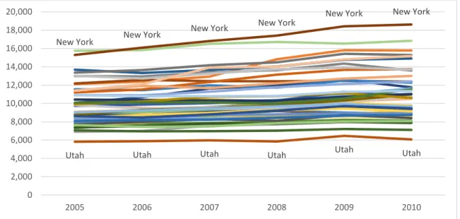
The mean of inflation-adjusted per-pupil education spending is $10,310 with a within standard deviation of $550 and an overall standard deviation of $2,400. The within standard deviation reflects how states increase education spending each year, by around $210 a year on average, once adjusting for inflation. In addition to yearly increases in spending on education, the overall variation between how much each state spends on education relative to other states is enormous. As discussed previously, the importance of per-pupil education spending (PPE) for migration outcomes has been recognized by past researchers, especially given the significant variation that exists between states in education outlays (Cebula, 2009).

(29)

29 provide an example of how different states fund education differently. Adjusted for inflation, New York increased their PPE by nearly $820 each year, or 6 percent of their 2005 spending, meanwhile Utah increased their PPE by only $141 each year, or 2.7 percent of their 2005 spending. Combining such distinct disparities in education spending with the understanding that high-income earners have more knowledge about education than other migrants contributes to education being a significant factor in migration outcomes. Well-informed individuals can relocate to benefit from educational advantages, and this effect is potentially even larger at the local level beyond merely the state level.

Figure 1 Per-Pupil Education Spending, 2005-2010 (in 2010 dollars)

Source: U.S. Department of Education

The mean of state budgets as a percentage of state GDP is 10.34%. The within standard deviation is 0.85, while the overall standard deviation is much higher at 2.81. States do not change their spending levels much over time; however, states have very different levels of spending compared to each other. Much like GDP per capita, states spend outlays in a relatively

New York New York

Utah Utah Utah Utah Utah Utah

0 2,000 4,000 6,000 8,000 10,000 12,000 14,000 16,000 18,000 20,000

(30)

30 fixed manner that results from obligations of governance such as Medicaid and corrections spending.

To demonstrate the types of changes to marginal tax rates that have historically occurred, Table 2 shows the six states that lowered their taxes by more than 1 percent. The only real outlier is Rhode Island, which was able to decrease taxes by 3.29 percentage points in part because their starting tax rates were higher than other states. The other 5 states only decreased taxes by 1-1.57 percentage points over 5 years, which represent particularly modest changes.

Table 2. States That Decreased Taxes by More than 1 Percent

State Tax Change (2005-2010)

Rhode Island -3.29

North Dakota -1.57

Nebraska -1.5

Ohio -1.27

Oklahoma -1.21

Utah -1.15

Source: The National Bureau of Economic Research

In contrast, six states increased their tax rates by more than 1 percentage point over the period from 2005-2010, as shown in Table 3. Again, Hawaii is an outlier which increased their taxes by 3.15 percentage points, while the other 5 states only increased their taxes by 1.23-2 percentage points. Regardless of whether taxes are increased or decreased, these data points indicate that state tax changes can be relatively large and are often gradually introduced over several years.

Table 3. States That Increased Taxes by More than 1 Percent

(31)

31

Hawaii _3.15

Illinois _2.00

Connecticut _1.70

Oregon _1.68

Maryland _1.43

New York _1.23

Source: The National Bureau of Economic Research

For several states, notably New York and North Carolina, tax rates fluctuated

significantly over the period 2005-2010. For instance, New York dropped their income tax rate from 7.74% down to 6.86% before raising it again to 8.98%. The rate was raised in 2009, which was a common theme among states which increased their tax rates, and many states raised rates to offset low revenue resulting from the 2009 Recession. For North Carolina, taxes were lowered from 8.5% to 7.83% before they were increased to 7.98% by 2010. While these fluctuations are relatively common, it is important to note that many of them do not change the marginal tax rates by more than one percentage point. For comparison, 17 states, including all of the states with no income tax, did not change their tax rates at all over the period studied.

(32)

32 correlation is -0.26, and this slightly negative correlation persists once no income tax states are removed, and the correlation becomes -0.30. The difference in signs and magnitudes

demonstrates that there is no clear, consistent relationship between migration and taxes using only correlations. In this way, simple analysis can be used by to create different scenarios in which taxes are both positively or negatively associated with net migration rates.

Table 4. Conditional Correlation with Net Migration

Analysis Condition Conditional

Correlation

Marginal Tax Rates -0.22

Marginal Rates Excluding States with No Income Tax 0.13

Average Taxes Paid as a % of Total Income -0.26

Average Taxes Paid as a % of Total Income Excluding States with No

Income Tax -0.30

Source: The National Bureau of Economic Research, IPUMS, Tax Foundation

Analyzing the data via regressions tells a more nuanced story. Previous regressions which did not control for state fixed effects do not answer the policy question of what happens if a state changes their tax rate while holding everything else constant. Table 5 summarizes each of the different regressions and ways of slicing the data. The four fixed effects regression types have an outcome variable of absolute net migration with a dependent variable of marginal tax rates, an outcome of net migration and total tax rates, an outcome of net migration as a rate and marginal tax rates, and an outcome of net migration as a rate and total tax rates.

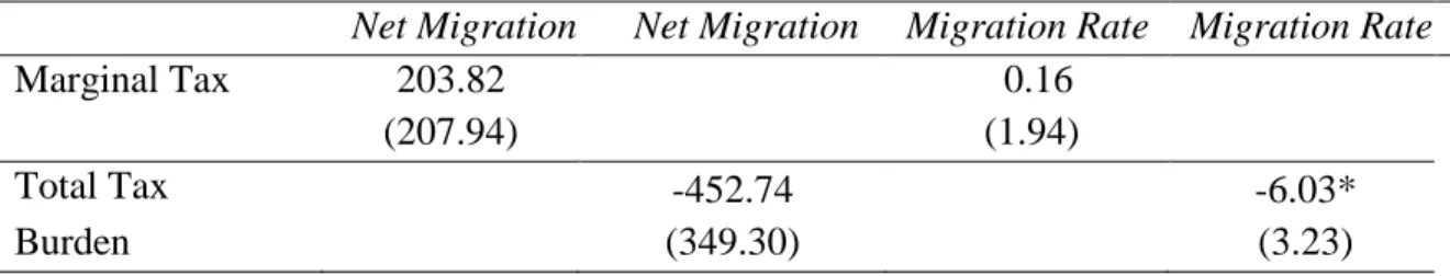
Table 5. Regression of Taxes on Net Migration (2005-2010)

Net Migration Net Migration Migration Rate Migration Rate

Marginal Tax 203.82 0.16

(207.94) (1.94)

Total Tax -452.74 -6.03*

(33)

33

State Budget as -223.59 -279.01 -3.47* -4.09**

% of GDP (209.58) 212.02 (1.95) (1.96)

Per-Pupil 387.90 527.06** -0.86 0.45

Education (241.49) (248.20) (2.25) (2.30)

GDP per Capita 198.65 -99.57 3.00 0.04

(744.08) (757.23) (6.93) (7.01)

Constant _-3658.49 _2160.63 _30.17 _93.77*

(4541.13) (5704.08) (42.28) (52.81)

R2 (within) 0.03 0.03 0.03 0.05

F for change in R2 0.63 0.55 0.47 0.20

Standard errors are reported in parentheses.

*, **, *** indicates significance at the 90%, 95%, and 99% level, respectively.

Note: Each regression has been controlled for year and state fixed-effects, but coefficients have not been included Note: Migration totals have been weighted using the ACS household weighting information

The most important takeaway is that total tax burden has a significant, negative migration rate per thousand residents of -6.03. This means that when the sum of all taxes excluding federal taxes is taken into account, higher taxes generally means more out-migration. To illustrate the full impact of taxes on migration, consider that the average state has approximately 110,588 individuals making over $100,000 per year. With an overall standard deviation of 97,000, most states have fewer than 304,000 high-income individuals each year. Taking into account the net migration rate per thousand, the results indicate that the average effect is about 6 residents per thousand. The effect of one overall standard deviation change in total tax burdens is equivalent to up to 1824 individuals leaving the state each year. This is a fairly significant number of high-income individuals who would be induced to move, but importantly, they do so as a reaction to their total tax burden, not simply their marginal tax rates. In this sense, it is possible that reducing the total tax burden residents face once sales tax, property tax, and local taxes are factored in can draw in residents.

State budget as a percentage of GDP has a negative and significant coefficient for

(34)

34 which have large budgets relative to their state economy attract fewer residents than states with smaller budgets. However, one could also interpret these results to mean that states with poor economies also tend to have lower GDPs, and states with poor economic conditions attract fewer residents. Additionally, much of state budgeted spending beyond education is not for public goods that benefit high-income Americans. Programs like Medicaid and prisons are significant in state level public spending terms, and states which spend more on these programs will have higher spending as a percentage of GDP. High-income earners aren’t attracted to states with large public spending beyond education, and may be deterred from relocating to states with high public spending.

In absolute terms, per-pupil education spending has a significant positive coefficient of 387-527 individuals into the state for each additional $1,000 in per-pupil education spending. This may mean that high-income earners are attracted to areas with good schools. It is also possible that, since using total taxes incorporates local spending and schools are funded significantly by local taxes, this coefficient is more likely to be significant due to variations in local spending. In particular, spending on public education is different from other forms of public spending because the children of high-income earners are much more likely to receive the

benefits of that specific public good. While increasing taxes alone might not attract high-income residents, if the higher taxes are associated with more spending on public education, then a significant number of high-income individuals may be motivated to relocate.

(35)

35 earners may focus on a particular industry or segment of the economy that is only a small portion of total GDP per capita. A state’s economic performance on this indicator tells us little about why high-income earners move; however, it is important that it is included in the regression to control for it as a possible factor.

The only significant variables are state budget as a percentage of GDP for migration rates, per-pupil education spending for net migration, and total tax burden for migration rates. Instead of a clear directional effect, the coefficients frequently change signs based on the types of taxes used and whether or not net migration is in absolute terms or a rate. This is similar to the conditional correlation results and suggests that there is no clear, one-directional relationship between taxes and migration. In the four regressions above, having higher or lower taxes in a state is not a significant determinant of the state’s ability to attract and retain residents in any meaningful way. Few of the predictors in these regressions are statistically significant, which suggests that marginal tax changes alone are ineffective at attracting residents.

Consider that the 95% confidence interval for marginal taxes is -3.66 to 3.97. This means that a one-percentage change in marginal taxes would still result in just 3 high-income individual moving into or leaving the state for every 1,000 high-income individuals residing in the state. That is an underwhelming 0.3% effect out of only high-income individuals, and an even smaller proportion of total residents in a state. This rate is very close to zero and suggests that, on a rate basis, marginal taxes have at best a negligible effect on net migration. This is consistent with the low absolute value for migrants apparent from the first regression and indicates that even large changes in tax rates do not result in significant migration impacts relative to other factors.

(36)

36 304,000 high-income individuals each year. The effect of a one percent change in marginal tax rates is equivalent to up to 48 individuals coming into or leaving the state each year. Since the confidence interval includes both directions, it is difficult to discern whether residents are entering or leaving a state due to these tax changes, further complicating whether taxes attract or repulse residents. States have an average of 6 million total residents, so the maximum effect of 48 individuals from one overall standard deviation change in marginal tax rates account for just a drop in the bucket in terms of the number of residents in the state. I conclude that the migration response for any reasonable tax change is very near zero, and the case for marginal tax rates having a significant determinant effect on migration is weak.

Discussion

For policymakers seeking to attract high income individuals, the results are not

particularly encouraging. The most viable policy mechanism is through education spending since per-pupil education spending is a significant predictor of net migration outcomes for total tax burdens. Still, spending an additional $1,000 on per-pupil education spending only bring in 387-527 individuals in absolute terms. These additional high-income individuals who move to or remain in the state as a result of the policy will not provide enough additional tax revenue to fund $1,000 in additional education spending on each student. Likewise, lowering public education spending is likely to result in lower net-migration rates.

(37)

37 wealthy job creators and entrepreneurs. Even if the largest effect from total tax burdens occurs and 1824 residents move in for each standard deviation change, these residents are not

significant enough to drive migration. Further, any attempt to lower taxes can be counteracted by neighboring states adjusting their tax rates to be more similar, and often this is the motivation we see from states when they adjust their rates. Taxes are primarily a tool for determining the

amount of revenue that states raise, and their effect on migration is much less significant than other factors.

The financials will vary from state to state, but in many cases the increased revenue from all taxpayers affected by higher tax rates will exceed the revenue lost from citizens leaving the state. While rhetoric about lowering tax rates to remain competitive and bring in residents may be true on a small level for the total tax burden, the cost associated with doing so would

outweigh the practical revenue benefits for public finance. Cutting taxes by one percentage point will almost certainly outweigh any additional revenue from new residents, although it is possible that these new residents are creating value for the state if they are significant job creators.

Furthermore, there is a beggar-thy-neighbor aspect of state tax rates in which states lower their tax rates to compete over the same residents. This process mostly benefits high-income

individuals since the majority simply end up paying lower taxes and do not migrate at all.

(38)

38 Chapter 5: Conclusions

While there have been a number of studies on the effects of taxation on behavior, no study to my knowledge has examined the effects of changes in state taxes on the migratory behavior of high income individuals. According to the Tiebout hypothesis, we should find a large and consistent effect from raising or lowering state tax rates on migration. Instead, I find that there is no statistically significant effect of marginal tax rates on net migration outcomes. There is a small, statistically significant effect from total tax burdens on net migration rates. Per-pupil education spending is a statistically significant determinant variable of net-migration outcomes. Attempts to attract new high-income residents as job creators and innovators through changes to state income tax rates is not a viable strategy, both in terms of revenue lost and the possibility that lower taxes will result in less spending on public education. My results suggest instead that providing high-quality education with high per-pupil expenditures is a much better way to attract these kinds of individual. Since my outcome variable was net-migration, this also suggests that per-pupil education spending may be more effective at retaining high-income individuals. Thus, not only may policies to provide quality education bring in new residents, they can also be seen as a valuable public good which helps to retain residents who might otherwise move.

Why might schools be a more effective policy tool for attracting high-income residents than taxes? One proposed mechanism is through saliency and variation – most parents are very aware of whether the schools in their area are good or not, and they also place a great deal of emphasis on sending their children to good schools because this is seen as a significant

(39)

39 schools are likely to provide a much better educational environment than the lowest quality public schools. The difference on life outcomes for those two types of education is much larger than the difference between paying 10.76% state income tax in Oregon and paying no income tax in Texas. Education quality variation also exists over a smaller geographic area. For instance, two schools across the same metropolitan area may have vastly different student profiles and outcomes for student achievement, and all that is required for a student to attend the better school is a move across town. Since exploiting tax rates requires residents to move across state lines, the costs are typically higher and will discourage citizens from exploiting differences. For both reasons of saliency and variation, high-income residents are more likely to choose their residency based on good schooling rather than whether or not they face a high tax burden in a state. In addition, well-funded education systems are more likely to develop citizens so that they are more attractive and capable to job creators in the future.

Spending on education is also different from other types of spending by state governments. In many cases, spending on other items is associated with a decrease in net migration, which may still indicate a preference. If high-income individuals tend to leave or avoid areas which have high public spending as a percentage of GDP, these individuals may have a preference against the provision of public goods. Since they do not receive many tangible benefits from the provision of certain public benefits, high-income individuals may be motivated to simply avoid states that spend a lot on public benefits. Further research that explores the attitudes of high-income earners towards public good provision may solidify the notion that these individuals have a preference for a low level of public goods provision.

(40)

40 federal tax rate schedule. For instance, even for an individual exploiting the largest moving advantage of going from 10.76% top marginal rate in Oregon to a 0% rate in Texas, this 10.76% difference pales in comparison to the 39.6% rate for federal taxes. While a particular high-income migrant might be able to reduce their combined federal and state top marginal burden from 50.4% to 39.6%, this only represents a 21% total savings. If state taxes were much higher and closer to the federal rate schedule, opportunities for tax savings would be much higher and the incentive to do so would be much greater. As of now, this incentive only exists in a small number of cases and the incentive is relatively small compared to the constant federal tax burden, which will remain the same regardless of the state of residence.

On the theoretical level, this is a unique application of the Tiebout hypothesis that expands upon traditional notions of voters. While the classic idea is that consumer-voters relocate to take advantage of the services provided and will gravitate towards low tax, low-service areas, my research suggests that in many states the opposite is also true. High-income earners, as a subset of the population seek out high levels of public provision of services such as education, potentially driving up taxes to provide funding for these services. In this way, high-income earners are the marginal consumer-voters that push equilibrium upwards to achieve a greater level of services. This new level of services attracts more high-income individuals, and thus perpetuates even higher levels of services in areas that have them.

I want to acknowledge that there are a variety of additional factors which affect migration but which were not considered for this paper. Namely, the distance traveled between two

(41)

41 take into account the average distance traveled to determine whether moving to a state bordering a migrant’s original state has a significant effect. Additionally, certain careers offer more

location flexibility that would allow a migrant to maintain their existing employment, and this could potentially have an effect on whether or not a high-income individual decides to migrate or not. The relatively large effect of total tax burdens compared to the effect of marginal tax rates demonstrates that total taxes are a better predictor of migration. Rather than state government worrying about their perceived competitiveness through marginal tax rates, making changes to the total tax burden by changing property taxes, sales taxes, or local taxes may provide better policy solutions to attract residents. Additional research which examines each of these types of taxes more closely could determine which area is most effective at causing net migration.

When determining a state tax rate, states must consider the empirical tradeoffs between attracting residents and raising revenue. In most cases, increasing taxes will raise revenue more than the loss from residents who leave the state, and decreasing taxes will lower revenue more than the influx of new residents. In this sense, states are not really competing to attract residents as the total flow of residents from one state to another is relatively small. Rather, states are merely choosing to raise or lower revenue as they see fit or to redistribute the sources of tax revenue away from the income tax and towards other means such as a state sales tax. Since only hundreds of residents per state make decisions each year based on changes in taxes, states would do best to focus on using state income taxes to raise however much revenue is deemed

(42)

42 References

Anderson, S. (2003, 2 14). Tax cut is on fast track to Richardson's signature. The Albuquerque Tribune, p. A1.

AP. (1992, 7 23). Bruce: TABOR aims to let people speak - Opponents rip his view of government. The Gazette, p. 3.

AP. (2006, 6 26). Session ends with budget, myriad legislation. The Westerly Sun, p. 3. Cebula, R. J. (2009). Migration and the Tiebout-Tullock Hypothesis Revisited. The American

Journal of Economics and Sociology, 68(2), 541-551.

Clark, D. E., & Hunter, W. J. (1992). The Impact of Economic Opportunity, Amenities and Fiscal Factors on Age-Specific Migration rates. Journal of Regional Science, 32(3), 349-365.

Conway, K. S., & Houtenville, A. J. (1998). Do the Elderly "Vote with Their Feet?". Public Choice, 97(4), 663-685.

Conway, K. S., & Rork, J. C. (2012). No Country for Old Men (Or Women) -- Do State Tax Policies Drive Away the Elderly? National Tax Journal, 65(2), 313-356.

Davies, P. S., Greenwood, M. J., & Li, H. (2001). A Conditional Logit Approach to U.S. State-to-State Migration. Journal of Regional Science, 41(2), 337-360.

Donahue, J. D. (1997). Tiebout? Or Not Tiebout? The Market Metaphor and America's Devolution Debate. The Journal of Economic Perspectives, 11(4), 73-81.

Feldstein, M., & Vaillant, M. (1998). Can State Taxes Redistribute Income? Journal of Public Economics, 68(3), 369-396.

Frank, J., & Frank, A. (2013, 7 16). GOP agrees on state tax plan - Republican leaders reach consensus on package to cut income taxes. The News & Observer, p. 1A.

Hotelling, H. (1929). Stability in Competition. The Economic Journal, 41-57.

Integrated Public Use Microdata Series (IPUMS). (2013, 11 21). Integrated Public Use

Microdata Series: census microdata for social and economic research. Retrieved from IPUMS USA: https://usa.ipums.org/usa/

Leachman, M., Mazerov, M., Palacios, V., & Mai, C. (2013). State Personal Income Tax Cuts: A Poor Strategy for Economic Growth. Washington, DC: Center on Budget and Policy Priorities.

Lyons, W., & Lowery, D. (1989). Governmental Fragmentation versus Consolidation: Five Public-Choice Myths about How to create Informed, Involved, and Happy Citizens.

(43)

43 Musgrave, R. A. (1939). The Voluntary Exchange Theory of Public Economy. The Quarterly

Journal of Economics, 53(2), 213-237.

PBS. (2012, 8 24). Tax Cuts, Deregulation Among Republican Economic Priorities for 2012 Election. Retrieved from PBS Newshour: http://www.pbs.org/newshour/bb/politics-july-dec12-tampa_08-24/

Percy, S. L., & Hawkins, B. W. (1997). Further Tests of Individual-Level Propositions from the Tiebout Model. APA, 54(4), 1156.

Percy, S. L., Hawkins, B. W., & Maier, P. E. (1995). Revisiting Tiebout: Moving Rationales and Interjurisdictional Relocation. Publius, 25(4), 1-17.

Preuhs, R. R. (1999). Policy Components of Interstate Migration in the United States. Political Research Quarterly, 52(3), 527-547.

Siegel, J. (2013, 11 1). State finances - House GOP on tax cut : Not so fast. The Columbus Dispatch, p. 1A.

Stoddard, M. (2006, 12 29). Governor calls tax cut crucial - State's competitive position is on the line, he says - Governor's proposal. Omaha World-Herald, p. 1A.

Tax Foundation. (2012, 10 23). State and Local Tax Burdens: All States, One Year, 1977 - 2010. Retrieved from Tax Foundation: http://taxfoundation.org/article/state-and-local-tax-burdens-all-states-one-year-1977-2010

Teske, P., Schneider, M., Mintrom, M., & Best, S. (1993). Establishing the Micro Foundations of a Macro Theory: Information, Movers, and the. The American Political Science Review, 87(3), 702-713.

The National Bureau of Economic Research. (2013, 11 21). Maximum State Income Tax Rates 1977-2011. Retrieved from The National Bureau of Economic Research:

http://users.nber.org/~taxsim/state-rates/

Thompson, J. (2011). The Impact of Taxes on Migration in New England. Political Economy Research Institute.

Thompson, J. (2012). Raising Revenue From High-Income Households: Should States Continue to Place The Lowest Tax Rate on Those With The Highest Incomes? Political Economy Research Institute, 1-16.

Tiebout, C. M. (1956). A Pure Theory of Local Expenditures. Journal of Political Economy, 64(5), 416-424.

U.S. Census Bureau. (2013). Public Education Finances: 2011. Washington, DC: U.S. Government Printing Office.

(44)

44 http://factfinder2.census.gov/faces/tableservices/jsf/pages/productview.xhtml?pid=ACS_ 10_1YR_B20001&prodType=table

U.S. Department of Commerce. (2013, 12 27). GDP & Personal Income. Retrieved from Bureau of Economic Analysis:

http://www.bea.gov/iTable/iTable.cfm?reqid=70&step=1&isuri=1&acrdn=1#reqid=70&s tep=1&isuri=1&7001=1200&7002=1&7003=200&7090=70

U.S. Department of Education. (2011). National Center for Education Statistics, Common Core of Data (CCD). Retrieved from National Public Education Financial Survey:

http://nces.ed.gov/ccd/stfis.asp

Vellequette, L. P. (2010, 12 31). Ohio enacts last phase of '05 income tax cut. The Blade, p. A1. Young, C., & Varner, C. (2011). Millionaire Migration and State Taxation of Top Incomes:

Evidence from a Natural Experiment. National Tax Journal, 64(2), 255-284. Retrieved from

Thesis

Table of Contents