The Built Environment, Spatial Variation in Fine Particulate Matter Concentrations, and Attributable Mortality: A Scenario-Based Land Use Regression Approach
Theodore James Mansfield
A thesis submitted to the faculty of the University of North Carolina at Chapel Hill in partial fulfillment of the requirements for the degree of Master of City and Regional
Planning in the Department of City and Regional Planning.
Chapel Hill 2012
ii
TABLE OF CONTENTS
LIST OF TABLES………..iv
LIST OF FIGURES………...v
LIST OF ABBREVIATIONS..……….…..vi
LIST OF SYMBOLS………..………...vii
ACKNOWLEDGEMENTS………..…………...…………...viii
ABSTRACT………...………..………...ix
CHAPTERS 1. INTRODUCTION………..……….……....1
2. BACKGROUND AND LITERATURE REVIEW Land Use Regression………..……….………...4
The Built Environment and Air Quality………..………….……...9
3. METHODOLOGY Overview of the Study Region………..………..………...15
The Triangle Regional Model………..………..………....18
Land Use Regression Model Selection…………..………....21
Land Use Regression Model Calibration………...………....25
Risk Assessment Model………...………..………....30
4. BASE CASE RESULTS Base Case Summary Statistics.….………...………...33
iii
Base Case PM2.5 Concentrations………..………….…….………....35
Base Case Attributable Mortality………..……….…….……...36
Discussion………..………..….…….………....39
5. SCENARIO MODELING Alternative Land Development Scenarios………..….…….……...43
Scenario Summary Statistics………...………...………....50
Scenario PM2.5 Concentrations………..….………..……...52
Scenario Attributable Mortality………..….……….………...55
Discussion………..….…….………...59
6. DISCUSSION AND POLICY IMPLICATIONS………...62
Policy Implications……..….…….………...65
7. CONCLUSIONS……….……...68
9. APPENDICES Appendix I: Annual Average PM2.5 Data and Discussion ………..…...69
Appendix II: Explanatory Variables ………..….………...80
Appendix III: Statistical Analysis………..….………...112
iv
LIST OF TABLES
1. Built Environment and Air Quality Literature………...10
2. North American Land Use Regression Studies……….23
3. Base Case Summary Statistics………..……….33
4. Attributable Deaths from PM2.5, 2010………..……….37
5. Model Error Terms………...………….41
6. Scenario Summary Statistics, Population Density……….50
7. Attributable Deaths from PM2.5, Scenario 1……….………….57
8. Attributable Deaths from PM2.5, Scenario 2……….……….59
v
LIST OF FIGURES
1. Coupled Model Research Schematic……….15
2. Study Area Overview……….16
3. Triangle Regional Model Schematic……….19
4. Location of Air Quality Monitoring Stations……….28
5. Predicted PM2.5 Concentrations, Base Case………..…….36
6. Estimated Deaths Attributable to PM2.5, 2010………...39
7. Population Density, Scenario 1………..46
8. Population change relative to the base case, Scenario 1………....47
9. Population Density, Scenario 2………..49
10. Population change relative to the base case, Scenario 2……….……….50
11. Predicted PM2.5 Concentrations, Scenario 1……….…………..……….53
12. Predicted PM2.5 Concentrations, Scenario 2……….………..…….54
13. Estimated Death Rate Attributable to PM2.5, Scenario 1……….55
vi
LIST OF ABBREVIATIONS CO Carbon monoxide
CO2 Carbon dioxide
GIS Geographic Information System HC Hydrocarbon
HIA Health impact assessment NO Nitrogen oxide
NO2 Nitrogen dioxide
NOx All mono-nitrogen oxides
O3 Ozone
PM Particulate matter
PM2.5 All particulate matter with a diameter less than 2.5 µm PM10 All particulate matter with a diameter less than 10 µm RR Relative risk
RTP Research Triangle Park SO2 Sulfur dioxide
vii
LIST OF SYMBOLS Microgram
Parameter coefficient for the nth model term Model error term
Coefficient of determination = Attributable mortality or morbidity
Baseline incidence, equal to baseline incidence rate (I0) multiplied by the potentially affected population (P)
viii
ACKNOWLEDGMENTS
I wish to acknowledge my committee for their support and willingness to share their expertise throughout the completion of this research. Special thanks are due to Dr. Paul
Voss for his valuable contributions to the statistical methods used in this research, Joe Huegy for his assistance with the Triangle Regional Model, and Monisha Khurana for
ix
ABSTRACT
THEODORE JAMES MANSFIELD: The Built Environment, Spatial Variation in Fine Particulate Matter Concentrations, and Attributable Mortality: A Scenario-Based Land
Use Regression Approach
1
Chapter 1: Introduction
Urbanization is occurring at a rapid rate across the globe. For the first time in human history, more than half of the world’s population lives in cities. In many developed countries, greater than 80% of the population lives in urban areas (The World Bank, 2011). The role of urban agglomerations as the dominant mode of human settlement provides a strong rationale for research on the impacts of urbanism on human health and well-being. However, many effects of large-scale urbanism on human well-being remain under-researched. Public health, broadly defined as “the science and art of preventing disease, prolonging life and promoting health through the organized efforts and informed choices of society, organizations, public and private, communities and individuals” is inherently linked to the environment in which we live (Winslow, 1920). Thus, the effects of urbanization on public health constitute an area of research that is relevant from both an academic and policy-making perspective. This research explores one of the many ways in which urbanization affects public health: fine particulate matter concentrations resulting from urban development and the health effects of exposure to fine particulate matter.
2
health focuses on the relationship between the built environment and air quality (see, for example, Frank et al. 2006). However, many existing studies of the built environment and air quality are limited to assessing aggregate emissions over large spatial scales (see, for example, Behan et al. 2008, Koracin et al. 2009). While important from a regional or global perspective, aggregate emission predictions are not useful in elucidating the impacts of pollutants on a local scale. The ability to predict local scale impacts is crucial in characterizing the public health ramifications of built urban forms. Furthermore, the literature on the built environment and air quality has generally relied upon gridded chemical fate and transport models with coarse spatial resolution (see Table 1). In response to this shortcoming in the literature, this research uses a land use regression model to predict air quality with higher spatial resolution than previous studies in order to explore the relationship between the built environment, local air quality, and human exposure to airborne contaminants. A risk assessment model is integrated into the research design to translate predicted local air quality into estimated health effects. Fine particulate matter, defined as particles suspended in the air with a diameter smaller than 2.5 µm and referred to as (PM2.5) is the environmental pollutant of interests in this study. Given the established health effects of PM2.5 are the demonstrated ability land use regression models to accurately model spatial variation in PM2.5 concentrations in the urban context (see, for example, Ross et al. 2007, Moore et al. 2007, and Henderson et al. 2007), PM2.5 is an appropriate pollutant for this study.
3
4
Chapter 2: Background and Literature Review
A growing body of literature exists exploring the relationships between the built environment and public health. A literature review of two primary bodies of research areas was undertaken:
1) Applications of land use regression to model local air quality; and
2) Existing research on the built environment and airborne emissions.
The health effects of chronic exposure to fine particulate matter are well-documented in the literature and thus are not reviewed separately here (see, for example, Dockery et al. 1993; Krewski et al. 2000; Laden et al. 2006; Pope et al. 1995, 2002). However, it should be noted that the presence of PM2.5 is highly correlated with the presence of other airborne pollutants, such as carbon monoxide (CO), hydrocarbon (HC), and nitrogen oxides (NOx) from mobile sources (Kunzli et al. 2000). Thus, the health effects of PM2.5 may be an effective proxy for the health effects of a wide variety of airborne contaminants and PM2.5 may therefore be an effective overall indicator of urban air quality.
Land Use Regression
5
While the term land use regression infers that only land use data may be in the regression model, the term is a misnomer - explanatory variables may include any data that are spatially distributed over the study area. In the urban context, predictor variables may include land use characterization, average daily traffic, population density, household characteristics, or a host of other built environment characteristics. Land use regression modeling has been used to predict spatially distributed concentrations of air quality indicators (Hoek et al. 2008).
Land use regression is a stochastic technique, thus land use regression models require local ambient monitoring data for model calibration. Local calibration accounts for factors such as regional background pollutant levels, average local meteorological conditions, and local automotive fleet composition (i.e., fuel mix, vehicle type mix, and fleet-average fuel efficiency). There is little consensus regarding the number of ambient monitoring stations required to effectively calibrate a model to local conditions (Hoek et al. 2008). While Hoek et al. note that a majority of studies use purpose-built networks to collect a large number of ambient condition observations, a number of studies have utilized fixed regulatory monitoring stations with a much smaller number of observations (see, for example, Moore et al., 2007; Ross et al. 2007).
6
scale, the computational and data requirements of such models make them infeasible for application across an urban area (see, for example, Zwack et al. 2011 and Greco et al. 2007). Furthermore, the computational complexity inherent in chemical fate and transport models has directly limited either the spatial resolution of grids or the geographic scale of analysis in other studies (Potoglou et al. 2005, Zwack et al. 2011).
A number of studies have explored the ability of land use regression techniques to accurately predict local air quality. A recent review yielded 25 studies (Hoek et al. 2008); a number of subsequent studies have been conducted since the 2008 review (see, for example, Hoek et al. 2011, Mao et al. 2012). Existing studies have shown that land use regression can accurately predict local air quality at high spatial resolution: studies in the literature report R2 values in the range of 0.6-0.7 (see, for example, Briggs et al. 2000, Hoek et al. 2008, and Hoek et al. 2011). Furthermore, comparative research has revealed that land use regression methods are able to model local air quality with accuracy equal to or exceeding that of chemical fate and transport models, thus achieving similar results using a less computationally expensive technique (Briggs et al. 2000, Cyrys 2005).
7
regression models to predict PM2.5 is the lack of spatially distributed monitoring stations that track PM2.5. Without these data, land use regression models may not be well calibrated to local conditions and will likely perform poorly.
Computational simplicity, the ability to predict air quality with high spatial resolution, and demonstrated accuracy in previous studies provide strong arguments for employing land use regression models when considering the effects of urban form on air quality and public health at the local scale. Henderson et al. echo this point, noting that “dispersion models that simulate pollution fate and transport can be useful, but are often infeasible at high spatial resolution throughout large areas” (Henderson et al. 2007, 2422). Land use regression, on the other hand, “can be used to predict concentrations at any spatiotemporal resolution within the framework of a Geographic Information System (GIS)” (Henderson et al. 2007, 2422). Marshall et al. also note that land use regression “is a hybrid empirical-statistical approach that combines concentration measurements with GIS maps, thereby offering a high degree of spatial resolution” (2009, 1753). Thus, existing studies present sufficient support for land use regression modeling as an effective tool for predicting local air quality at fine spatial resolution.
8
revealed the potential of locally calibrated models to predict local air quality accurately if transferred even to contrasting urban areas (Briggs et al. 2000). An additional study supports the transferability of land use regression models, stating that “…there is only a small penalty in limiting land use regression models to a consistently defined set of predictor variables” (Vienneau et al. 2010). This study is somewhat limited in that Vienneau et al. only analyzed the transferability of NO2 and PM10 models between Great Britain and the Netherlands. Poplawski et al. also conclude that the transferability of models between cities in Canada is relatively high (Poplawski et al. 2009); however, Jerrett et al. find that a model calibrated in the European context does not explain spatial variation in Hamilton, Ontario, Canda (Jerrett et al. 2005). Thus, it seems that land use regression models are generally transferable within the same broad societal and regulatory context, subject to routine local calibration. Studies of the New York metropolitan area and the Los Angeles urban area have broadly demonstrated the ability of land use regression modeling to predict local air quality with sufficient accuracy (R2 = 0.62 and 0.69, respectively) in the North American context (Ross et al. 2006; Moore et al. 2007). Therefore, a locally calibrated model that has been shown previously to be effective in the United States may be transferable to other similar metropolitan areas in the United States.
9
land use regression models are a linear combination of variables, including a model constant. Common explanatory variable in studies predicting PM2.5 concentrations include traffic density and/or intensity, land use classification, and population density (see, for example, Ross et al. 2006, Henderson et al. 2007, Moore et al. 2007, and Hoek et al. 2011). Research suggests that the accuracy of land use regression is not significantly affected if the form of a model that has been calibrated in a similar context is adopted in a new urban area and re-calibrated using local ambient monitoring data (Poplawski et al. 2009). Thus, it can be inferred that a land use regression model consisting of a linear combination of traffic density and/or intensity, land use classification, and population density is generally applicable in the Triangle Region, subject to calibration using local ambient monitoring data.
The Built Environment and Air Quality
10
Table 1. Built Environment and Air Quality Literature
Study Study
Type
Geography Emissions and Air
Quality Model Types
Independent Variable(s) Dependent
Variable(s)
Andrews, 2008
Non-statistical
New Jersey Fleet-average MPG Community typology per the rural-to-urban transect
Aggregate: CO2 equivalents Bart, 2010
Cross-sectional
EU member states
Aggregate member state emissions
Change in artificial area , per capita GDP
Aggregate CO2
Behan et al., 2008
Scenario Ontario, CA MOBILE5C (no dispersion)
Scenarios Aggregate: HC, NOx, CO
Borrego et al. 2006
Scenario Idealized city MEMO/MARS (dispersion; 2km grid cells)
Idealized city form Air quality: Ozone, NO2
Exposure: Ozone, NO2 Clark et al.,
2011
Cross-sectional
111 US urban areas
N/A: Monitoring data Population density, population centrality, transit supply
Population-weighted concentrations: PM2.5, O3
De Ridder et al., 2008
Scenario Ruhr area, Germany
MIMOSA; AURORA (dispersion, 2km grid cells)
Scenarios Aggregate: CO, NOx, VOC, PM
Air quality: O3, PM10 Exposure: O3, PM10 Frank et al.,
2000
Cross-sectional
King County, WA
MOBILE5a Household density, work employment density, home employment density, distance to work, census block density
Per household: NOx, CO, VOC
Frank et al., 2006
Cross-sectional
King County, WA
MOBILE6.2 Composite walkability index Per capita: NOx, VOC
Ewing et al., 2007
Scenario United States VMT elasticities Scenarios Aggregate: CO2
Koracin et al., 2009
Scenario Southwest California
EMFAC2002 + CAMx dispersion model w/ 5x5 km grid
Scenarios Aggregate: CO, NOx, SO2, VOC, PM (total); Air quality: O3
Levy et al., 2010
Projection 83 US urban areas
MOBILE6, source-receptor matrix (dispersion model)
Business-as-usual Premature deaths: NOx, SO2, PM2.5
Manins et al., 1998
Scenario Melbourne, AUS
Land-use-transport model; dispersion model
Scenarios Aggregate: CO2 Air Quality: O3 Exposure: O3, PM10 Marshall et
al., 2005
Scenario Idealized city Single compartment model (uniform concentration)
Scenarios Air quality: CO Exposure: CO
Marshall, 2008
Scenario US (regional) Population density-VKT elasticity, fleet-ave. MPG
Scenarios Aggregate: CO2
Marshall et al., 2009 Cross-sectional Vancouver, B.C., CA
NO: land-use regression; O3: spatial interpolation
Neighborhood walkability Air quality: NO, O3
Potoglou et al., 2005
Scenario Hamilton, Ontario, CA
MOBILE5C + Line source dispersion model (CALINE-4) and universal kriging
N/A – not linked to urban form descriptively
Air Quality: CO
Song et al., 2008
Scenario Austin, TX MOBILE 6.2 and CAMx (O3 only)
Scenarios Aggregate: NOx, VOC Air quality: O3
Stone et al., 2007
Scenario Midwestern US
MOBILE 6 (no dispersion)
Scenarios Aggregate: CO, NOx, PM, VOC
Stone et al., 2009
Scenario Midwestern US
Fleet-average MPG (tract level)
Scenarios Aggregate: CO2
11
12
A persistent shortcoming of this literature is the lack air quality predictions with high spatial resolution. As illustrated in Table 1, nearly all studies that consider air quality as an outcome rely upon gridded chemical fate and transport models with coarse spatial resolution. Two exceptions exist in the literature reviewed. An analysis of Vancouver, British Columbia, Canada, in terms of walkability and air quality used land use regression to predict air quality at high spatial resolutions (Marshall et al. 2009). Additionally, a study of transportation emissions in Hamilton, Ontario, Canada uses a line source dispersion model and universal kriging to predict air quality at high spatial resolution. While this study does not use land use regression, the combination of a line source dispersion model and universal kriging improves spatial resolution compared to peer studies. However, this study is limited because the CALINE-4 line source model used is computationally limited to analyze only twenty (20) links and twenty (20) receptor nodes simultaneously; therefore, a generalized road network is used for analysis and universal kriging is applied between receptor points, thus ignoring potentially important spatial variation between receptor points (Potoglou and Kanaroglou 2005). This research builds upon the existing body of work by applying a land use regression model to alternative land development scenarios, thus allowing for air quality and exposure predictions with high spatial resolution without needing to make simplifying assumptions due to computational limitations.
13
14
Chapter 3: Methodology
15
Figure 1. Coupled Model Research Schematic
Overview of the Study Region
16
Figure 2. Study Area Overview
17
Raleigh, the University of North Carolina at Chapel Hill, Duke University in Durham, and North Carolina State University in Raleigh. The region is highly auto-dependent, with a private vehicle mode share (including carpooling) of 89.7% as estimated by the 2010 American Community Survey 5-year estimates (U.S. Census Bureau, 2010b). Although fixed-route transit service is planned for the near future, the Triangle Region currently relies solely on bus transit and is served by several local transit agencies, several university-affiliated transit agencies, and one regional transit agency. The Triangle Region suffers from intermittent poor air quality. In 2010, 117 days were recorded with a moderate Air Quality Index and five (5) days were considered “unhealthy for sensitive groups” (United States Environmental Protection Agency, 2010). Particulate matter concentrations are generally moderate and have been decreasing in the region significantly over time (United States Environmental Protection Agency, 2012).
18
established legal precedent within the state. The built environment characteristics of the Triangle are emblematic of many urban agglomerations across the nation; thus, this “urban laboratory” presents an opportunity to investigate the connections among urban from, air quality, and health effects of human exposure to particulate matter from both an academic and a policy-making perspective.
The Triangle Regional Model
19
trucks. The model includes an iterative feedback mechanism to ensure accurate convergence (Triangle Regional Model Service Bureau, 2011). The TRM is executed within TransCAD 5.0 build 1880. The complete TRM structure is presented in Figure 3.
20
The TRM offers the most accurate available prediction of transportation network usage within the Triangle Region, providing estimated traffic flows on a large percentage of streets throughout the region. However, the model is unable to predict intra-zonal trips and trips on minor streets, likely resulting in systematic under-prediction of short distance motorized and active mode trips. Land use regression is not sensitive to absolute quantities but rather the difference in quantities across space; therefore, systematic under-prediction of vehicle-kilometers traveled is not necessarily detrimental to the land use regression models’ predictive abilities. Additionally, unpredicted intra-zonal active mode trips may be associated with significant inhalation rates; thus, the inability of the TRM to forecast intra-zonal trips limits the ability of the risk assessment model to assess PM2.5 exposure in certain populations. While the TRM is able to predict network usage at three time periods, this study will use the AM peak as a proxy to represent overall variation spatial variation in vehicle-kilometers travelled throughout the day. While this method does not directly predict vehicle-kilometers for the entire day, it does represent expected spatial variability in vehicle-kilometers travelled and therefore is appropriate for use in the land use regression modeling framework.
21
accurately adjust to large-scale changes in demographic information. Simply stated, the model is able to predict transportation behavior only in scenarios that are roughly demographically equivalent to the base case.
Land Use Regression Model Selection
Rather than fully specifying a unique land use regression model for the Triangle Region, an existing model form is adopted and calibrated using local ambient air quality monitoring data. This methodology is consistent with other land use regression transferability studies undertaken in the literature (Poplawski et al. 2009); however, it is a simplification of the general case of land use regression. In the general case, stepwise regression is used to select the most effective explanatory variables from an extensive list of potential explanatory variables. Transferring an existing model allows for specification of a much smaller set of potential explanatory variables, thereby eliminating significant data processing requirements and the need for stepwise regression to select final explanatory variables for the model. Within the North American context, transferability studies have supported the applicability of carefully specified models to similar urban areas (Poplawski et al. 2009).
22
23
Table 2. North American Land Use Regression Studies
Study Geography Dependent
Variable
Model Parameters R2 Value
Gilbert et al. 2005
Montreal, CA NO2 Distance to highway + Traffic count nearest highway + Length highways (100 m) + Length major roads (100 m) + Length minor roads (500m) + Open space (100 m) + Population Density (2000 m)
0.55
Kanaroglou et al. 2005
Toronto, CA NO2 Distance to nearest expressway + Expressway (200m) + Local roads (300m – 500m) + Major roads (500m) + Open space (400m) + Dwelling density (2000m)
0.63 Adj: 0.61
Gonzalez et al. 2005
El Paso, TX NO2 Distance to US-Mexico border + Distance to highway + Elevation
0.81
Smith et al. 2005
El Paso, TX NO2 Elevation + Traffic intensity (1000 m) + Population density + Distance to border + Distance to petroleum facility
>0.90a
Smith et al. 2005
El Paso, TX VOC Altitude + Traffic (1000 m) + Distance to highway + Population density + Distance to border + Distance to petroleum facility
>0.90a
Ross et al. 2006
San Diego County, CA
NO2 Traffic density (40-300 m) + Traffic density (300-1000 m) + Road length (40 m) + Distance to coast
0.79
Ross et al. 2007
New York City, NY
PM2.5 Traffic (500 m) + Population (1000 m) + Industrial land use
(300 m)
0.64
Ryan et al. 2007
Cincinnati, OH
Elemental carbon
Altitude + Truck density (400 m) + Length bus routes (100 m)
0.75
Moore et al. 2007
Los Angeles, CA
PM2.5 Traffic density (300 m) + Industrial land use (5000 m) +
Government land area (5000 m)
0.69
Henderson et al. 2007
Vancouver, CA
NO2 Length expressway (100 m) + Length expressway (1000 m) + Length major roads (200 m) + Population density (2500 m) + Commercial areas (750 m) + Altitude + X-coordinate
0.56
Henderson et al. 2007
Vancouver, CA
NO Length expressway (100 m) + Length expressway (1000 m) + Length major roads (200 m) + Population density (2500 m) + Altitude + Y-coordinate + X-coordinate
0.52
Henderson et al. 2007
Vancouver, B.C., CA
PM2.5 Commercial area (300 m) + Residential area (750 m) +
Industrial area (300 m) + Elevation
0.52
Henderson et al. 2007
Vancouver, B.C., CA
PM2.5b Length expressway (1000 m) + Length major roads (100 m)
+ Distance highway + Open area (500 m)
0.39
Wheeler et al. 2008
Windsor, Ontario, CA
NO2 Distance to Ambassador bridge + Length expressways and highways (50 m) + Length of major roads (100 m)
0.77
Wheeler et al. 2008
Windsor, Ontario, CA
VOC (Benzene)
Length of major roads (100 m) + Length of expressways and primary highways (50 m) + VOC emission (4000 m) + VOC emission (3000 m)
0.73
Wheeler et al. 2008
Windsor, Ontario, CA
VOC (Toluene)
Distance to Ambassador bridge + Length of major roads (200 m) + Length of primary highways (100 m) + VOC emission (1000 m) 0.46 Poplawski et al. 2009 Victoria, B.C., CA
NO2 Population density (2500 m) + Length of highways (1000 m) + Length of major roads (200 m) + Elevation + Commercial land use (750 m) + Length of highways (100 m)
0.58
Poplawski et al. 2009
Victoria, B.C., CA
NO2 Length of major roads (500 m) Length of highways (750 m) + Industrial land use (500 m) + Elevation
0.61
Poplawski et al. 2009
Seattle, WA NO2 Population density (2500 m) + Length of highways (100 m) + Length of major roads (200 m) + Length of highways (1000 m) + Commercial land use (750 m) + Elevation
0.65
Poplawski et al. 2009
Seattle, WA NO2 TRANS (750 m) + Length of major roads (300 m) + Length of highways (100 m) + Pop. density (2500 m)
0.72
a Artificially high as reported from Generalized Additive Model using 16 degrees of freedom with 22 observations b
24
As seen in Table 2, land use regression models used to predict particulate matter concentrations in the literature generally rely upon one or more explanatory variables that represent transportation network usage within some buffer of the prediction cell, and one or more explanatory variable that describe land use within a defined buffer from the prediction location. Population density and elevation are also used as explanatory variables in some published models. The preliminary land use regression model for the Triangle Region contains explanatory variables that describe transportation network usage, land use characteristics, and population density within defined buffer sizes. Buffer sizes are not assumed to be constant across all explanatory variables. Variation in elevation in the Triangle Region is generally minimal; therefore, it is not included as an explanatory variable in the preliminary model for the Triangle Region. The model takes the same general form as published models; that is, a linear combination of explanatory variables with a model constant. The preliminary model form is depicted in [2] below; descriptions of model parameters follow:
Ɛ [1]
β0 is a model constant that captures regional background concentrations; that is,
PM2.5 mass concentrations that are unexplained by local variation in land use, traffic density, or population density;
25
IND_LU explains local variation in PM2.5 mass concentrations resulting from proximity of the prediction location to land uses that emit primary PM2.5 or PM2.5 precursors. This variable is expressed as a percentage of the land within the buffer area that is designated for manufacturing, industrial, or warehouse use;
POP_DEN explains local variation in PM2.5 mass concentrations associated with population density within the buffer. Although this parameter may not be completely independent of other explanatory variables, it has been demonstrated in several studies to be independent of traffic intensity and/or or land use explanatory variables; and
Ɛ is a standard error term that is checked for normality, heteroscedasticity, independence, and spatial autocorrelation to ensure that the specified model does not violate the underlying assumptions of multiple linear regression.
Land Use Regression Model Calibration
26
are maximized to ensure accurate calibration; that is, the additional uncertainty introduced in inferring PM2.5 concentrations from PM10 concentrations at the additional monitoring site is outweighed by the extra spatial information gained at this location. Additionally, not all monitoring stations report an annual average PM2.5 concentration for 2010. However, all sites displayed strong linear trends over time; thus, all data are imputed to 2010 using monitoring station-specific linear regression models. This procedure is documented in Appendix I. While examples of spatiotemporal land use regression models exist in the literature (see, for example, Mao et al. 2012), this model is calibrated only for 2010. The stochastically determined model constant assumes constant regional background over time and vehicle-kilometers travelled parameter coefficient implicitly assumes vehicle fleet characteristics such as fuel mix and fuel efficiency; thus, the calibrated model is only applicable for its calibration year, assuming vehicle fleet characteristics and regional background change over time.
27
Gaussian distribution and meaningful variation exists amongst monitoring stations for most explanatory variables. See Appendix II for greater detail.
28
Figure 4. Location of Air Quality Monitoring Stations
29
independence. While both total vehicle-kilometers travelled and population density exhibit some level of correlation with annual average PM2.5 concentrations at various buffer sizes, industrial land use exhibits no correlation with annual average PM2.5 concentrations. Additionally, inclusion of the industrial land use variable does not improve model performance, as assessed using the coefficient of determination (R2). Therefore, the industrial land use variable is not included in the final land use regression model for the Triangle Region. Exploratory analysis of the explanatory data reveals that Station 37-04 (near Pittsboro) and Station 37-20 (south of the outer beltline in Raleigh) are problematic. Both of these stations are surrounded by predominantly rural land uses and are generally not located proximate to significant links in the regional transportation network. Thus, the data for explanatory variables for both of these stations are outliers compared to the rest of the sample. Despite the small number of observations, these observations are removed from the set of observations used to calibrate the final model due to the extremely low values observed for all model parameters. Conceptually, these stations capture regional background concentrations of PM2.5; therefore, comparison of the calibrated model constant with observed values at these monitoring stations provides a check of model performance. See Appendix II for additional detail.
30
dependent variable. Consistent with existing literature, the coefficient of determination is considered sufficient to test this assumption. Secondly, observations are assumed to be spatial independent of one another. The Moran’s I test is used to test for spatial autocorrelation of observations. Thirdly, model parameters are assumed to be linearly independent of one another. Model parameters are plotted against one other to ensure independence. Statistical analysis is presented in Appendix III.
Risk Assessment Model
31
associated with predicted PM2.5 concentrations above the regional background (i.e., above the predicted model constant) is calculated at the block group level. The function used to quantify the burden of disease attributable to outdoor air pollution is described below in [2]:
[2]
= Attributable mortality or morbidity
Baseline incidence, equal to baseline incidence rate (I0) multiplied by the potentially affected population (P)
Concentration-response coefficient from epidemiological studies Change in concentration of the pollutant of interest
The World Health Organization has proposed calculating the attributable fraction (AF) of total burden of disease from a specific risk to be:
[3]
= Relative risk
Relative risk is commonly calculated as:
[4]
Thus, equation [2] may be written as follows:
[5]
32
thus, a dense block group suffering from poor ambient air quality conditions is considered “worse” than a sparsely populated block group with the same predicted ambient conditions. Thus, this analysis is implicitly human-centric and is biased to consider human health impacts as more important than regional or global environmental impacts; however, this is roughly in agreement with the general regulatory ideology for environmental protection in the United States.
33
Chapter 4: Base Case Results
Base Case Summary Statistics
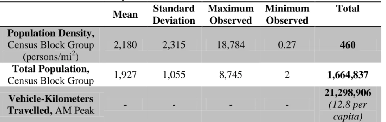
Summary statistic for the base case presented in Table 3. Population density statistics are presented at the Census block group level while vehicle-kilometers travelled are shown in the aggregate (i.e., total forecast vehicle-kilometers travelled for the study region). Per capita vehicle-kilometers travelled are also displayed for illustrative purposes.
Table 3. Base Case Summary Statistics Mean Standard
Deviation Maximum Observed Minimum Observed Total Population Density,
Census Block Group (persons/mi2)
2,180 2,315 18,784 0.27 460
Total Population,
Census Block Group 1,927 1,055 8,745 2 1,664,837
Vehicle-Kilometers
Travelled, AM Peak - - - -
21,298,906
(12.8 per capita)
34 Calibrated Model
PM2.5 concentrations in the study area are estimated by the following equation:
[6]
Predicted annual average PM2.5 concentration,
µgm-3
= Total vehicle-kilometers travelled during the AM peak within a 1,000 meter buffer of the estimation point, thousands of vehicle-kilometers travelled
Population density within a 1,500 meter buffer of the estimation point, thousands of persons per square mile
35
inclusion of the parameter, POP_DEN_1500m is left in the model despite statistical insignificance. See Appendix III for the outputs of statistical analysis.
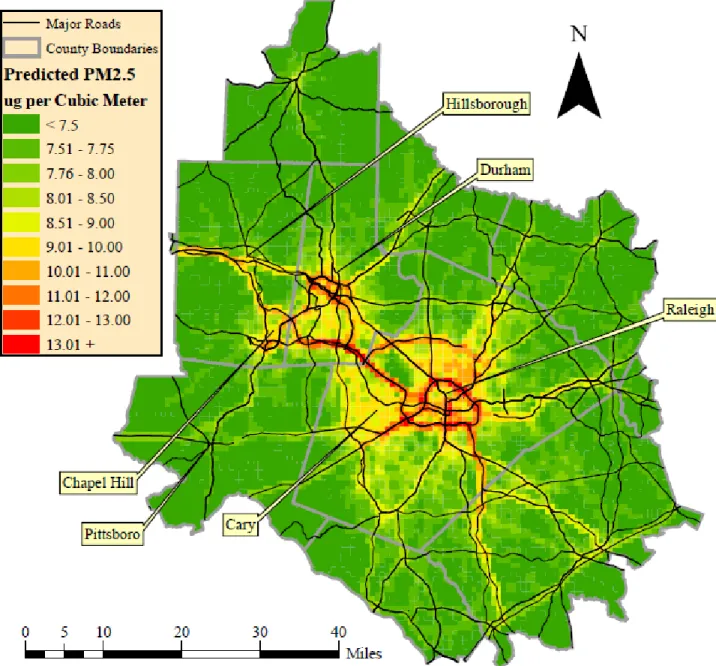
Base Case PM2.5 Concentrations
Predicted annual average PM2.5 concentrations in the Triangle area are depicted in Figure 5. As expected, areas of higher predicted annual average PM2.5 concentrations are spatially correlated with significant links in the transportation network. The spatial distribution of predicted annual average PM2.5 concentrations illustrative the highly localized impacts associated with regional transportation patterns, particularly along primary transportation links such as I-40. A notable shortcoming of the model is its inability to predict variation in local air quality associated with point-source emissions, general industrial land use, and special-case uses such as airports. This limitation is attributable to the lack of sufficient such uses near ambient air quality monitoring stations in the Triangle Region. Nonetheless, the model demonstrates that regional travel parts have a significant impact on local air quality in the Triangle Region.
36
region, 0.62% of the predicted vehicle-kilometers travelled during the AM peak occur within the 1,000 meter buffer extending from the centroid of this cell.
Figure 5. Predicted PM2.5 Concentrations, Base Case
Base Case Attributable Mortality
37
regarding the health effects of PM2.5 to estimate total deaths attributable to PM2.5 in the study region in 2010. County-level deaths from all-cause mortality and associated death rates for 2009 are presented in Table 4 (North Carolina State Center for Health Statistics, 2012). While the Base Case study year is 2010, county-level health data are not yet available for 2010; therefore, it is assumed that 2010 death rates are equal to 2009 death rates. 2009 population estimates are taken from the 5-year estimates of the 2009 American Community Survey (U.S. Census Bureau, 2009). The relative risk for all-cause mortality related to exposure to PM2.5 is taken from Pope et al., who report a mean relative risk of 1.06 for all-cause mortality per 10 µg m-3 increase in annual average PM2.5 concentrations (2002). The model constant in the calibrated air quality model is assumed to represent regional background (i.e., variation unassociated with the model explanatory variables); therefore, in order to estimate deaths attributable to PM2.5 from local sources, the model constant is subtracted from predicted PM2.5 concentrations in the study region prior to estimating attributable deaths in the risk assessment model. In total, the model estimates 82 deaths in 2010 attributable to PM2.5 above regional background.
Table 4. Attributable Deaths from PM2.5, 2010 County 2009 Total
Deaths
2009 Population
2009 Death Rate
2010 Estimated Deaths Attributable to PM2.5
Alamance 1,411 144,769 0.009747 <<1a
Chatham 570 61,444 0.009277 <1a
Durham 1,688 256,296 0.006586 20
Franklin 469 57,201 0.008199 <1a
Granville 491 55,670 0.008820 <1a
Harnett 849 108,885 0.007797 <1a
Johnston 1,168 156,888 0.007445 3a
Nash 913 92,814 0.009837 <<1a
Orange 670 124,503 0.005381 6
Person 398 37,301 0.010670 <1a
Wake 4,150 828,759 0.005007 50
TOTAL Attributable Deaths: 82 a
38
39
Figure 6. Estimated Deaths Attributable to PM2.5, 2010
Discussion
40
insignificance of this model parameter, POP_DEN_1500m is not removed from the model because of the theoretical basis for its inclusion and improved observed performance of the model resulting from its inclusion. First, while the VKT_1000m parameter captures a significant portion of vehicle-kilometers travelled within the study area, the TRM is limited to predicting traffic flows only on primary and secondary streets. Thus, may neighborhood streets are unaccounted for in this parameter. The inclusion of household population density helps capture variation in neighborhood-level vehicle kilometers traveled, assuming that households have roughly similar trip generation characteristics on the aggregate. Second, the model parameter has been found to be significant in a number of existing studies that used a greater number of observations (see, for example, Ross et al. 2007, Moore et al. 2007). Third, household density may serve as a very rough proxy for capturing general variability in land use intensity at the neighborhood level that is not captured by vehicle-kilometers travelled, which is predicted using data at the regional scale. Fourth, the population density data seem to be independent of the vehicle-kilometers travelled data (see Appendix II); therefore, the data are capturing some meaningful variation, albeit partially random variation, that helps predict PM2.5 concentrations in the study area. Finally, including the POP_DEN_1500m improves the coefficient of determination from 0.8781 (0.7969 adjusted) to 0.8257 (0.7667 adjusted).
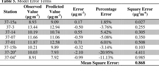
41
emissions not accounted for in the model and may thus be a spatial anomaly compared to other monitoring stations in the Triangle Region. Table 5 reports the model estimated values at each monitoring station as well as the error in the estimate at each monitoring station.
Table 5. Model Error Terms Station
Observed Value (µgm-3)
Predicted Value (µgm-3)
Error (µgm-3)
Percentage Error
Square Error (µg2m-6)
37-15a 8.93 9.09 0.17 1.85% 0.027
37-3 13.44 12.94 -0.50 -3.76% 0.255
37-14 10.19 10.74 0.55 5.42% 0.305
37-07 11.66 11.06 -0.59 -5.08% 0.350
37-01 11.87 12.58 0.71 6.01% 0.508
37-15b 10.21 9.89 -0.32 -3.14% 0.103
37-20a 10.03 7.93 -2.10 -20.95% 4.411
37-04a 8.91 7.92 -0.99 -11.13% 0.985
Mean Square Error: 0.868 a Observed values removed for model calibration, see Appendix II for rationale
A fundamental assumption of multiples linear regression is the independence of model parameters; thus, it is critical to consider the independence of the selected explanatory variables. As illustrated in Figure 42 in Appendix II, the variables VKT_1000m and POP_DEN_1500m are independent of each other around monitoring stations. It should be noted that inclusion of the two rural monitoring stations biases the relationship as both parameters are near zero around these two stations (see Figure 40,
42
43
Chapter 5: Scenario Modeling
Alternative Land Development Scenarios
The alternative land development scenarios are developed to meet the assumption of ceteris paribus – scenarios are developed so that the only variable that changes is the spatial distribution of employment and housing within the study area. Thus, the transportation network is constrained to the base case network in both scenarios. While transportation behavior changes as a result of land use changes, the rules that govern the generation, assignment, characterization, and distribution of trips on the network remain constant. Study area population and demographic information are held constant in the aggregate. It should be noted that it is critically important to maintain aggregate demographic consistency through all scenarios, as the TRM utilizes logit models to predict transportation demand that are based on and calibrated using demographic information. Thus, any significant departures from the base case aggregate demographic profile of the population undermines the predictive ability of the TRM significantly. This process is somewhat problematic because population and demographic information are stored independently at the aggregate at the TAZ level; therefore, demographic shifts must be accounted for when population is re-distributed amongst TAZs.
44
should not be compared to the base case in a contemporary lens. Rather than representing alternative futures, they are an attempt to represent what the Triangle may look like today with a history of different land development policies. Therefore, although the scenarios may appear draconian in comparison to the current development pattern of the Triangle, they are intended to represent a development path entirely independent of the development path the Triangle has historically followed. Overall, although the magnitude of change in the alternative scenarios is extreme, they are intended to represent a radically different confluence of past development decisions in the Triangle and are thus intended to be somewhat disconnected from the realities of the Triangle as it exists today.
Scenario 1: A History of Smart Growth represents an alternative present for the Triangle highly influenced by the principles of compact development, growth management, and land conservation. Areas of existing density are made much denser while existing households and employment are completely removed from many rural areas. Thus, this scenario represents a Triangle in which the full gamut of land development policy instruments, such as density incentives, transfer of development rights, and urban growth boundaries, had been used to centralize development in constrained, targeted growth areas. Once more, this scenario is not necessarily intended to be realistic through the lens of the region’s contemporary policy context; rather, it is designed to represent a development path independent of the path the Region has followed.
45
46
47
Figure 8. Population change relative to the base case, Scenario 1
48
locations remain relatively concentrated in the core of the region. Thus, this scenario should theoretically greatly increase regional vehicle-kilometers travelled while dispersing both household locations and the concentration of vehicle-kilometers travelled across the study region.
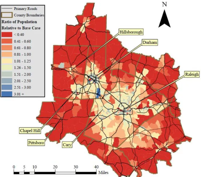
In order to generate this scenario, population is iteratively removed from the densest quintile of TAZs to the least dense individual TAZs in the study region. A maximum threshold of population density, defined as the highest observed population density in the central quintile of TAZs in terms of population density, is assumed to represent the highest development intensity in this scenario. This density threshold is 1,120 persons per square mile. Thus, population is removed from all TAZs with population densities that exceed this threshold value. Population removed from these TAZs is moved to all TAZs (excluding employment-only TAZs) based on the total number of residents that may be added to each TAZ before reaching the defined population density threshold. Thus, population is redistributed with a bias towards rural development. TAZs that have the lowest observed population density in the base case have the greatest number of redistributed residents. As previously mentioned, employment is left unaltered in this scenario.
49
per square mile (~1.75 persons per acre). Figure 10 illustrates the “hollowing out” of established urban cores that is intentionally magnified in this scenario.
50
Figure 10. Population change relative to the base case, Scenario 2
Scenario Summary Statistics
Summary statics comparing the base case and both scenarios are presented in Table 6.
Table 6. Scenario Summary Statistics, Population Density Scenario
Mean Group Population
Density
Standard Deviation, Block Group Population Density
Maximum Block Group Population
Density
Base Case 2.180 2,315 18,784
Scenario 1:
Smart Growth 2,495 2,613 16,421
Scenario 2:
51
52 Scenario PM2.5 Concentrations
53
Figure 11. Predicted PM2.5 Concentrations, Scenario 1
54
Thus, while dispersing population across the study area reduces PM2.5 “hotspots,” the regional average PM2.5 concentration, and therefore aggregate emissions, are increased in this scenario. The policy implications of this conclusion are intriguing and are discussed in greater detail Chapter 6.
55 Scenario Attributable Mortality
The risk assessment is applied to each scenario to determine the combined effect of changing land use patterns and predicted air quality on all-cause mortality attributable to PM2.5. It should be noted that this analysis assumes that 2009 death rates obtained from current (i.e., base case) conditions are applicable to the scenarios despite changes in land use (see Table 7 and Table 8).
56
57
Table 7. Attributable Deaths from PM2.5, Scenario 1 County 2010
Population 2009 Death Rate 2010 All-cause Mortality
2010 Estimated Deaths Attributable to PM2.5
Alamance 2 0.009747 <<1 <<1a
Chatham 12,612 0.009277 117 <1a
Durham 319,909 0.006586 2,107 32
Franklin 16,420 0.008199 135 <1a
Granville 9,162 0.008820 81 <1a
Harnett 8,416 0.007797 66 <1a
Johnston 95,496 0.007445 711 2a
Nash 259 0.009837 <<1 <<1a
Orange 113,252 0.005381 609 7
Person 11,526 0.010670 123 <1a
Wake 1,002,592 0.005007 5,020 65
TOTAL Attributable Deaths: 107 a
Attributable deaths only in the portion of the county in the study area
58
Figure 14. Estimated Death Rate Attributable to PM2.5, Scenario 2
59
the TRM predicts trips in some TAZs. Additionally, the larger geographic size of rural TAZs magnifies trip underproduction in the TRM resulting from its inability to predict intra-zonal trips. While these limitations do temper the results of Scenario 2 to some degree, the general conclusion of the scenario is still valid – strategies that reduce exposure to PM2.5 by locating households away from significant transportation corridors may be beneficial from a purely public health perspective. The policy implications of this conclusion are discussed in greater detail in Chapter 6.
Table 8. Attributable Deaths from PM2.5, Scenario 2 County 2010
Population 2009 Death Rate 2010 All-cause Mortality
2010 Estimated Deaths Attributable to PM2.5
Alamance 4 0.009747 <<1 <<1a
Chatham 117,384 0.009277 1,089 2a
Durham 175,179 0.006586 1,153 9
Franklin 110,524 0.008199 906 2a
Granville 70,841 0.008820 625 1a
Harnett 70,214 0.007797 548 1a
Johnston 217,528 0.007445 1,620 5a
Nash 11,431 0.009837 112 <1a
Orange 160,241 0.005381 862 4
Person 80,780 0.010670 862 1a
Wake 568,157 0.005007 2,845 22
TOTAL Attributable Deaths: 47 a
Attributable deaths only in the portion of the county in the study area
Discussion
60
the base case while Scenario 1 increases the standard deviation, indicating that compact growth increases local variation in PM2.5 concretions despite improving regional air quality. The apparent health effects of reduced density represent a Faustian bargain of sorts. While attributable mortality is reduced in Scenario 2, vehicle kilometers travelled are increased and regional air quality suffers. Thus, policy that aims to reduce the human health impacts of urbanization by decreasing density may be fundamentally misguided. Furthermore, the results of this analysis are predicated on a bias towards improved human health. While clearly a laudable policy goal, human health should be viewed in a holistic context and should consider the relevant tradeoffs. Thus, increased land consumption, increased aggregate emissions, decreased opportunities for physical activity, and ecosystem impacts that may result from low density urban forms should be considered in conjunction with human health impacts of air pollution in making rational policy choices. While characterization of these tradeoffs is beyond the scope of this analysis, consideration of these tradeoffs is needed to evaluate the ultimate policy implications of this research.
61
Scenario 2. Considering the lumpy nature of investments in transportation infrastructure, this result provides a strong rationale for increased consideration of the public health impacts of regional-scale transportation investments. While land use patterns may alter both local air quality and attributable mortality, the magnitude of these changes (and perhaps even the direction of change) may largely be defined by the existing system of infrastructure in the region. From a more abstract perspective, regional transportation systems may define a set of rules by which air quality and exposure pathways change is response to changes in land use. Thus, a region may be significantly constrained in its ability to address the public health impacts of PM2.5 by the existing regional transportation system.
Table 9. Summary of Results
Base Case Scenario 1: Smart Growth
Scenario 2: Sprawl Total vehicle-kilometers traveled 21,298,906 20,195,098 26,662,932
Change, relative to base case - - 5.18% + 25.19%
Average Predicted PM2.5
Concentration
7.84 7.81 7.93
Change, relative to base case - + 2.36% + 3.93%
Standard Deviation, PM2.5
Concentration
0.90 0.97 0.83
Change, relative to base case - + 7.78% - 7.78%
Maximum Predicted PM2.5
Concentration
15.62 16.04 14.41
Change, relative to base case - + 2.69% - 7.75%
Estimated Attributable Deaths, 2010 82 107 47
Change, relative to base case - + 29.9% - 42.6%
Average Attributable Mortality Rate 5.38 5.89 4.70
Change, relative to base case - + 9.48% - 12.6%
Maximum Attributable Mortality Rate
19.72 26.62 17.86
62
Chapter 6: Discussion and Policy Implications
63
this research suggests that compact development alone should not be considered an appropriate policy instrument for reducing the environmental burden of disease from fine particulate matter in urban areas.
Conversely, the results of this study should not be considered supportive of decentralization as a means of reducing the public health impacts of urbanization. Across all modeled conditions, regional mobility patterns result in highly localized air quality impacts – health effects are only of concern when population happens to be co-located with such impacts. Complete avoidance of areas with locally poor air quality due to regional mobility is not a feasible policy option. Furthermore, existing urban forms wherein high population density areas are located within close proximity to regional transportation corridors present an obvious barrier to the avoidance of areas with poor local air quality attributable to mobile source emissions. Additionally, this research does not consider the potential health benefits of compact development, such as increased physical activity attributable to the increased utility of active modes. Thus, while the research does not support compact development as a means of achieving improved human health outcomes, this research does not necessarily support the corollary. The conclusions of this research are also constrained to consider only direct health outcomes, while reduced transportation demand may be associated with a host of other indirect benefits to human health, including climate change mitigation and improved ecosystem health.
64
outcomes of urban development policy and the development of “ready for practice” tools to help decision makers consider complex and multi-faceted problems with non-intuitive outcomes. The result is particularly relevant considering the formative nature of Health Impact Assessment (HIA) in the United States – while the HIA process is maturing, methodologies often rely on qualitative judgment and the intuition of decision makers. Evidence suggesting the presence of non-intuitive relationships thus provides critical support for additional academic enquiry into the complex relationship between the built environment, transportation behavior, and public health impacts.
As previously mentioned, this research also may suggest that lumpy transportation investments may define the rules by which land use, transportation behavior, air quality, and public health interact. Despite radical land use changes in the analyzed scenarios, the location and degree to which PM2.5 “hotspots” were above regional average concentrations amongst scenarios are remarkably consistent. Thus, the large-scale nature of transportation investments may undermine the ability of decision makers to positively affect health outcomes via other policy interventions, such as compact growth. Therefore, this research provides clear support for the application of quantitative, scenario-based analysis when assessing the health impacts of large transportation investments that may fundamentally alter the future of a region and the ability of local policy interventions to affect meaningful change towards positive health outcomes.
65
scenario, demographic information is held constant, and the same regional transportation demand model is applied across all scenarios. Both scenarios are still influenced by entrenched behaviors and values and provide residents with the same basic mobility choice set. Thus, the conclusions of this research are very much contextualized to the region and are not supportive of a “one size fits all” approach to reducing the health impacts of transportation in a general sense. An effective set of policy instruments to reduce the health impacts of transportation in the Triangle would not necessarily be effective in other metropolitan areas across the country; however, this analysis builds on the understanding of the relationships among the built environment, air quality, and human health impacts and provides a strong rationale for considering human health effects in holistic discussions regarding regional policy goals relating to environmental and health outcomes.
Policy Implications
66
particulate matter is an equally sound policy goal. While the results of this analysis are not generally transferable, generalized policy recommendations are not possible. However, the research framework is illustrative of the type of analysis that should be conducted when balancing regional and local goals regarding human and environmental health.
While compact growth may be effective in reducing per capita vehicle-kilometers travelled and per capita emissions of particulate matter, increased density in and of itself is not an effective policy approach to reduce the population burden of disease attributable to human-generated atmospheric emissions. The effectiveness of other policy strategies, such as the provision of mass transit, community design to encourage zero-emission transportation modes such as walking and biking, and market pricing mechanisms for automobile mobility are not considered in this research but may be effective in improving both regional air quality and reducing the public health impacts of human-caused atmospheric emissions. The research design presented in this analysis is capable of exploring additional policy combinations, a potentially valuable future contribution to the body of knowledge considering the potential of the effect of multiple policy interventions to be greater than the sum of individual effects. An extension of the research framework presented in this research could easily gauge the effectiveness of a variety of combinations of policy instruments and infrastructure investments, such as increased density in conjunction with investment in fixed transit systems and road pricing or increased mixing of uses in conjunction with increased parking costs.
67
68
Chapter 7: Conclusions
69
Appendix I: Annual Average PM2.5 Data and Discussion
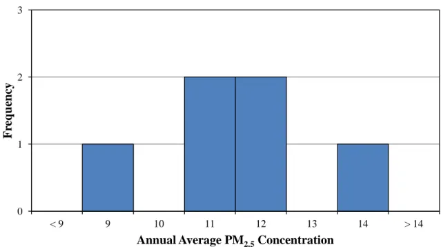
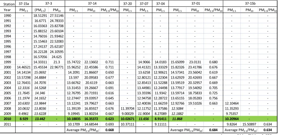
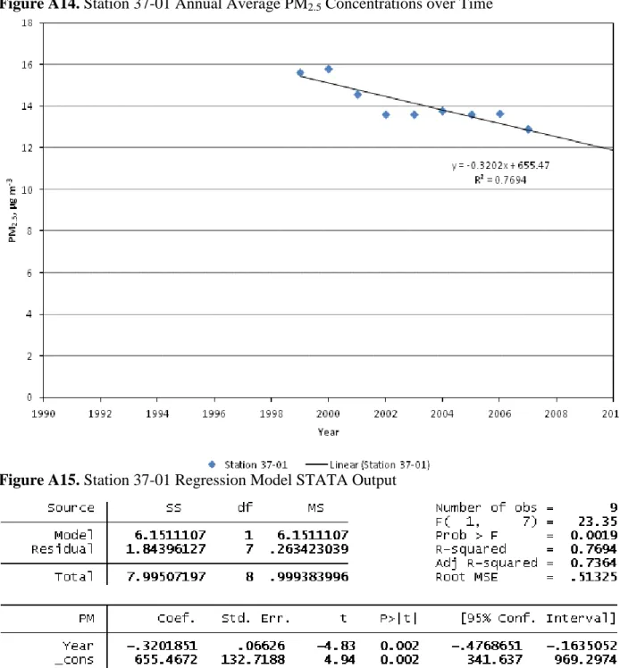
This section contains additional detail on monitoring stations, observed PM2.5 data, and interpolation techniques used to translate observed data into 2010 PM2.5 concentrations. Table A1 contains monitoring station summary information, Figure A1 and A2 presents the distribution of observed 2010 average PM2.5 concentrations (all observations and observations with stations 37-20 and 37-04 removed, respectively), Table A2 provides time series data for each monitoring stations. Figures A3-A17 provide time series plots of observed data and linear regression models for each monitoring station as well as statistical analyses of each regression model. The slope of all regression models are significant at 95% confidence with the exception of station 37-3, which is significant at above 85% confidence (p = 0.111 for the slope and p = 0.098 for the constant) and station 37-15b, which is significant at above 90% confidence (p = 0.055 for the slope and p = 0.054 for the constant). No regression model is presented for station 37-20 due to the low number of observations over time (n = 4).
70
Figure A1. Histogram, 2010 Annual Average PM2.5 Concentration Observations (all observations)
Figure A2. Histogram, 2010 Annual Average PM2.5 Concentration Observations
(stations 37-20 and 37-04 removed) 0
1 2 3 4
< 9 9 10 11 12 13 14 > 14
F re q u en cy
Annual Average PM2.5 Concentration
0 1 2 3
< 9 9 10 11 12 13 14 > 14
F re q u en cy