Vol. 4, No. 3, pp 156-166 Fall 2010
A Set of Algorithms for Solving the Generalized Tardiness Flowshop
Problems
Farhad Ghassemi-Tari1, Laya Olfat2
1Department of Industrial Engineering, Sharif University of Technology, Tehran, Iran [email protected]
2School of Management, Alameh-Tabatabie University, Tehran, Iran [email protected]
ABSTRACT
This paper considers the problem of scheduling n jobs in the generalized tardiness flow shop problem with m machines. Seven algorithms are developed for finding a schedule with minimum total tardiness of jobs in the generalized flow shop problem. Two simple rules, the shortest processing time (SPT), and the earliest due date (EDD) sequencing rules, are modified and employed as the core of sequencing determination for developing these seven algorithms. We then evaluated the effectiveness of the modified rules through an extensive computational experiment.
Keywords: Flowshop, Total tardiness, Intermediate due dates
1. INTRODUCTION
Meeting job due dates is one of the scheduling criteria most frequently considered in practical problems. Among these criteria, the most applicable performance measure is the minimization of the total tardiness (Lauff, and Werner 2004). In traditional flow shop models the work in a job is broken down into separate tasks called operations, while each operation of a job is performed at different machine in a unidirectional precedence structure. By unidirectional structure we mean that for each operation after the first there is exactly one direct predecessor and for each operation before the last there is exactly one direct successor. The shop contains m different machines and each job consists of m operations each of which requires a different machine. The machines in a flow shop can thus be numbered 1, 2, … m; and the operations of job j numbered (1, j), (2, j)… (m, j), so that they correspond to the machine required. For the traditional models with the total tardiness minimization objective, there is a given due date for completion of each job (last operation of each job), and the tardiness of a job is defined as the amount of time by which the completion of the last operation of a job exceeds its associated due date. In real world problems, however there is a considerable situation in which there is a due date for each intermediate operation of a job, and there exist a penalty associated with the tardiness of each intermediate operation of a job. The existence of these intermediate due dates distinguishes a new version of flow shop model which
Corresponding Author
Ghassemi-Tari and Olfat (2004) named it as “the generalized tardiness flow shop model”. Their justification for choosing this name is based on the fact that by assigning a large value to each intermediate due date (except the due date of the last operation of each job) the traditional tardiness flow shop model is acquired.
In the flow shop problem, there are n! job sequences, possible for each machine, and as many as (n!)m schedules. Among these schedules if we consider those by which the same job sequence occurs on each machine we will have the case of the permutation scheduling. In case of the permutation scheduling our effort for finding the best schedule is limited to the search for only n!
schedules (Baker, 1974). This paper considers the permutation scheduling of the generalized tardiness flow shop scheduling model.
Survey of the flow shop models reveals that there are limited researches addressing minimization of the total tardiness problems. Even in those we have found a few number of researches dealing with the tardiness flow shop problems with the intermediate due dates.
An early research considering the generalized tardiness flow shop is the work conducted by Ghassemi-Tari and Olfat (2004). In their paper two heuristic algorithms were developed for solving the generalized version of tardiness flow shop problems. They extended the traditional tardiness flow shop models by considering a due date for completion of each operation in an n jobs m
machine flow shop model. They modified the concept COVERT (Carroll, 1965) for the generalized version of the flow shop tardiness model and employed this concept for developing their algorithms. The efficiency of the developed algorithms was reported through their computational experiments.
Another research considering the intermediate due date flow shop is the work of Takaku and Yura (2005). In this research a simple method developed for solving a production schedule problem in which jobs are dispatched on to the idle machine tools. The method provides a schedule for a flow shop problem with the due dates related criteria. The production schedule is made as a job arrives and the completion time of a job is not determined till the job is selected as the next job on an idle machine. Then, online scheduling methods have been developed, in which the production schedule is made as a job arrives and it is clarified that the method is better than FIFO rule for the shops with heavy workload.
Bulbul, Kaminsky and Yano (2004) considered the problem of scheduling customer orders in a flow shop with the objective of minimizing the sum of tardiness, earliness (finished goods inventory holding), and intermediate (work-in-process) inventory holding costs. They formulated this problem as an integer program, and developed several heuristic algorithms to minimize the total cost. Their algorithms are basically are formed by combining two different lower bounds on the optimal integer solution, together with intuitive approaches for obtaining near-optimal feasible integer solutions. Through a computational study they demonstrated that their algorithms have a significant speed advantage over alternate methods. Their method yields good lower bounds, and generates near-optimal feasible integer solutions for problem instances with many machines and a realistically large number of jobs.
Ghassemi-Tari and Olfat (2007) developed four heuristic algorithms for solving the tardiness flow shop problems with the intermediate due dates. They modeled the problem of finding the best schedule of a set of projects as a generalized tardiness flow shop problem. They then developed a set of heuristic algorithms which are based on the concept of “apparent tardiness cost” (ATC). The
efficiency of their algorithms was compared with the existing algorithms and showed superiority in terms of the closeness to the optimal solutions.
Considering the intermediate due date tardiness as a special form of flow shop models, there are some other special versions dealing with the tardiness of flow shop models. A hybrid flow shop scheduling is one of the special types of the flow shop models in which the intermediate stages are considered. Lee and Kim (2004) suggested a branch and bound algorithm for a two-stage hybrid flow shop scheduling problem for minimizing total tardiness. In another research attempts, Chio, Kim and Lee (2005) considered total tardiness scheduling problem for the hybrid flow shop in which a set of orders with reentrant lots are scheduled. There are some other works dealing with the tardiness hybrid flow shop, such as works conducted by Lin and Liao (2003), and Gupta et al. (2002). Some other tardiness scheduling problems have considered batch processing of jobs which are presented in (Yeh and Alahverdi, 2004, and Bilge et al., 2004).
In this paper we considered the problem of scheduling jobs in the generalized tardiness flow shop problem with the total tardiness criteria. Some simple rules such as the SPT, and the EDD rules are modified and applied as the sequencing rules for obtaining the best permutation schedule of the problem. We then evaluated the effectiveness of the algorithms for obtaining the near optimal solution of the problem. We also evaluated the relative effectiveness of the developed algorithms. The relative effectiveness of the algorithms is measured by the extent their solution diverges from the best solution obtained by one of the seven algorithms.
2. NOMOCULTURES
The following notations are used throughout this section:
n Number of the jobs
m Number of the operations (machines)
pij Amount of processing time required for operation j of job i
dij Due date for operation j of job i
p[i]j Amount of processing time required for operation j of the job in the position i of a sequence
d[i]j Due date for operation j of the job in the position i of a sequence
TPi Summation of all the operations processing time for job i
TP[i] Summation of all the operations processing time for the job in the position i of a sequence
ECi Estimated completion time of job i
EC[i] Estimated completion time of the job in the position i of a sequence
rij Rank of job i on machine j
TRi Total rank of job i on machine j
SRj A sequencing rule to be applied on machine j
3. MODIFICATIONS OF SIMPLE RULES
In this section we will present the algorithms based on a set of factors consists of the jobs processing times, due dates, and combination of the processing times and due dates.
SPT Rule Algorithm
By applying this rule we simply determine the job sequence one machine at time with the shortest processing time rule. For example considering the jth machine, jobs are sequenced according to
p[1]j p[2]j p[n]j. Through this process we determine m different schedules. We now determine another sequence using the rule of shortest total processing time ((TP[1] TP[2] TP[n] ). Now by having m + 1 different schedules, we calculate the total tardiness of all the developed schedules and we select the final schedule with the smallest total tardiness among the m + 1 schedules. This rule determines the final sequence through the following algorithmic steps:
Step 1: Let j = 1.
Step 2: Sequence jobs in non-decreasing order of pij(p[1]j p[2]j p[n]j) on machine j.
Step 3: Define a permutation schedule on all machines using this sequence and calculate the total tardiness of all the jobs.
Step 4: If j = n, go to step 5, otherwise let j = j + 1, and go to step 2.
Step 5: Sequence jobs in non-decreasing order of TPi (TP[1] TP[2] TP[n] ). And define a permutation schedule on all machines using this sequence and then calculate the total tardiness of all the jobs.
Step 6: Select the final schedule with the smallest total tardiness among the m + 1 schedules, and stop.
EDD Rule Algorithm
By applying this rule we also determine the job sequence one machine at time with the earliest due date rule. For example considering the jth machine, jobs are sequenced according to d[1]j d[2]j d[n]. Through this process we determine m different schedules. Now by having m different schedules, we calculate the total tardiness of all the developed schedules and we select the final schedule with the smallest total tardiness among the m schedules. This rule determines the final sequence through the following algorithmic steps:
Step 1: Let j = 1.
Step 2: Sequence jobs in non-decreasing order of dij(d[1]j d[2]j d[n]j).
Step 3: Define a permutation schedule on all machines using this sequence and calculate the total tardiness of all the jobs.
Step 4: If j = n, go to step 5, otherwise let j = j + 1, and go to step 2.
Step 5: Select the final schedule with the smallest total tardiness among the m schedules, and stop.
SCT Rule Algorithm
This rule is similar to SPT, but for generating the first m schedules, instead of using the individual job processing time on each machine, we consider the total processing time of a job on the previous operations as an estimate for the job ready time and we add this time to the job processing time on a specific machine to find an estimated completion time of that job on that specific machine. Then we sequence jobs on that specific machine according to the shortest completion time. After determining a sequence on a specific machine, we use this sequence as a permutation schedule for all the machines. Considering one machine at a time, we determine m different schedules. Now by having
m different schedules, we calculate the total tardiness of all developed schedules and we select the final schedule with the smallest total tardiness among the m schedules. This rule determines the final sequence through the following algorithmic steps:
Step 1: Let
j
1
,
calculate the estimated completion time of all jobs on machine j as ni p EC
j
k ik
i 1,2,
1
.
Step 2: Sequence jobs on machine j according to a non-decreasing order of ECi (EC[1] EC[2] EC[n]).
Step 3: Define a permutation schedule on all machines using this sequence, and designate it as schedule j, then calculate the total tardiness of schedule j.
Step 4: If j = m, go to step 5, otherwise let j = j + 1, and go to Step 2.
Step 5: Select the final schedule with the smallest total tardiness among the m schedules, and stop.
4. DEVELOPMENT OF RANKING RULES ALGORITHMS
In this section we propose a set of algorithms, called ranking rules algorithms, which select the position of each job in the final sequence by considering its total ranking. To determine a rank for each job, we first generate m (or m + 1) different schedules on m machines based on some of the previously proposed rules. Then we assign the rank of k on job i where it has the position k in the sequence on machine j; rij = k where i = [k] on machine j. The total rank of a job is then determined as sum of its ranking in all m (or m + 1) sequences. The general procedure of all the ranking rules algorithms can be summarized by the following algorithmic steps:
Step 1: Let j = 1.
Step 2: Find a schedule in machine j according to rule SRj (RSPT, REDD, RSCT, RSPTEDD). Step 3: Assign the rank k to the job i; rij = k for job i = [k] i1,2,,n.
Step 4: If j = m, go to step 5, otherwise let j = j + 1, and go to step 2.
Step 5: Let ( ) 1,2, , . 1
1 1
n i
r or r TR
m
j ij m
j ij
i
Step 6: Determine the final permutation schedule by sequence of the jobs according to non-decreasing order of TRi (TR[1] TR[2] TR[n]).
Using the above procedure, we can have the following four ranking rules algorithms:
RSPT Rule Algorithm -This algorithm employs the SPT sequencing rule for SRj.
REDD Rule Algorithm - This algorithm employs the EDD sequencing rule for SRj.
RSCT Rule Algorithm - This algorithm employs the SCT sequencing rule for SRj.
RSPTEDD Rule Algorithm - This algorithm employs both the SPT and the EDD sequencing rule
for SRj and determines the total rank of each job by sum of its ranks among the 2m schedules.
5. COMPUTATIONAL EXPERIMENTS
We implement extensive numerical experiments to evaluate the effectiveness of the proposed algorithms. To show the effectiveness of the proposed algorithms in obtaining the optimal solution as well as comparing their relative effectiveness, computational experiments are conducted with a
variety of randomly generated test problems. In this section we first describe the mechanism of generating the test problems, and then we will present the experimental results.
5.1. Generation of the test problems
We employed the same concepts of generating the test problems, commonly have been used in the similar experiments. For each test problem with the size of n jobs and m operations, we used a uniform distribution with the rage [1-10] to generate pij's. The operations due dates are generated in two steps. In the fist step the due date of the last operation (dim) is generated using the following uniform distribution:
dim U[(1 - TF - RE/2)C, (1 - TF + RE/2)C]
Where TF is the due date tightness parameter, RE is the range adjusting parameter, and C is defined as follows:
n
i im m
j ij
i p p
C
1 1
1 } { min
Then we use dim to generate all other dij's as follows:
) 1 ( )
1
(
i j i i jij
d
p
d
,where
i = dim /TPi.
We let R = 0.02, and we generated 36 mid-size scenarios through the combinations of two different values to m, six different values of n, and three different values of TF. We then used different random number seed to generate 40 test problems to evaluate the effectiveness of the proposed algorithms in obtaining the optimal solution. In each scenario, all 40 test-problems are solved via total enumeration and the proposed algorithms, and total tardiness of each problem is determined by both methods. We then defined the measure of effectiveness of each algorithm in each scenario, as the deviations of its average solutions from average of the optimal solutions.
Similarly we generated 96 larger -size scenarios through the combinations of four different values of m, eight different values of n, and three different values of TF. Again we generate 40 test problems to evaluate the relative effectiveness of the proposed algorithms.
In each scenario, all 40 test-problems are solved by the proposed algorithms, the average of total tardiness obtained by of 40 test-problems are determined. We used the algorithm with the minimum average solution in each scenario as the index algorithm, and then defined the relative measure of effectiveness of each algorithm, as the deviations of its average solution from the average solution of the index algorithm.
5.2. Computational results
We now present the results of the computational experiments. To compare the relative effectiveness of the developed algorithms we generated several classes of the test problems with three different levels of toughness. We employed a factor called TF to differentiate the toughness of the generated
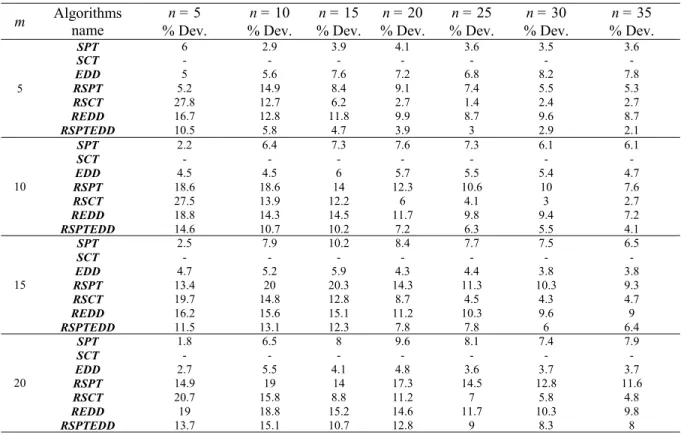
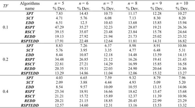
test problems. We then assigned three values to this toughness factor, namely .01, 0.2, and 0.4. Table 1 demonstrates the relative effectiveness of the algorithms for toughness factor of 0.1. In this table we classified 32 different test problem scenarios, and solved 40 problems for each scenario. The 32 flowshop test problem scenarios are consist of four different of values for the number of machines, m = 5, m = 10, m = 15, and m = 20, and eight different values for the number of jobs, n = 5, n = 10, n = 15, n = 20, n = 25, n = 30, n = 35, and n = 40. The results of these experiments show that the one of the developed algorithm called SCT performs better than all other developed algorithms. Similar experiments are conducted for TF = 0.2, and TF = 0.4. Table 2 and Table 3 demonstrate the experimental results of the test problems with TF = 0.2, and TF = 0.4 respectively. As it is shown from these three tables, SCT performs best among all the other developed algorithms. We also evaluated the effectiveness of the developed algorithms for obtaining the optimal solution. To evaluate the performance of the developed algorithms in obtaining the optimal solution, we generated several classes of the test problems with three different toughness levels. We classified 18 different test problem scenarios, and solved 40 problems for each scenario. The 18 flowshop test problem scenarios are consist of three different of values for the toughness factors, TF = 0.1, TF = 0.2, and TF = 0.4, and six different values for the number of jobs, n = 5, n = 6, n = 7, n = 8, n = 9, and n = 10, when the number of machines is consider to be 5, m = 5. We solved the test problems via the developed algorithms and through total enumeration. We then determined the percentage of the deviations of the objective function values obtained by each algorithm from the optimal objective function value for each scenario. Table 4 illustrates the value of these deviations. Again from this table, it is shown that SCT performs better than all the other developed algorithms in obtaining the optimal solution. Similar experiments are also conducted for the flowshop test problems with eight machines, m = 8. Table 5 illustrates the value of these deviations. Again from this table, it is shown that SCT performs better than all the other developed algorithms in obtaining the optimal solution. It is to be noted that, for the larger test problems the optimal value could not be obtained in a reasonable computational time.
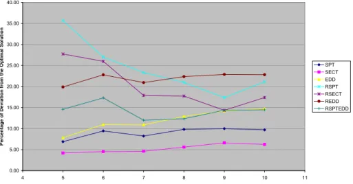
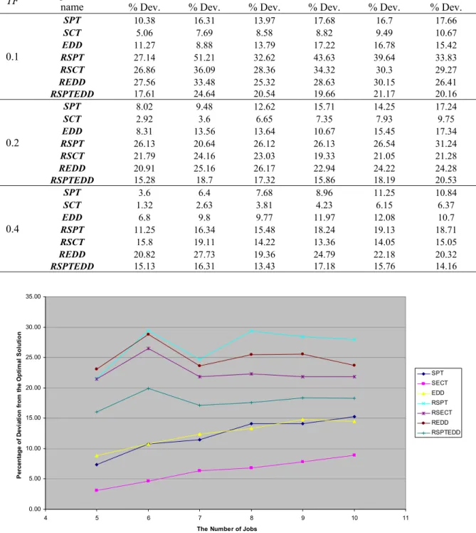
For a better illustration of the effectiveness of the developed algorithms in obtaining the optimal solution, we developed two graphical representations of the results. Figure 1 and Figure 2 are depicting the effectiveness of the developed algorithms in obtaining the optimal solution for the values of m = 5, and m = 8, respectively when we averaged the objective function values of each scenario over the toughness factor values.
Figure 1 Effect of the number of jobs on the effectiveness of algorithms (m = 5, averaged of TF's)
0.00 5.00 10.00 15.00 20.00 25.00 30.00 35.00 40.00
4 5 6 7 8 9 10 11
The Number of Jobs
P
erc
en
ta
ge
of De
vi
at
ion from the
Opti
ma
l
S
o
lu
ti
on
SPT SECT EDD RSPT RSECT REDD RSPTEDD
Table 1 The relative effectiveness of the algorithms for TF = 0.1
m Algorithms name % Dev. % Dev. % Dev. % Dev. % Dev. % Dev. % Dev. % Dev. n = 5 n = 10 n = 15 n = 20 n = 25 n = 30 n = 35 n = 40
5
SPT 3.1 3.4 5.3 3.7 3.6 3.6 4.2 3.8
SCT - - -
EDD 2.2 7.1 7.7 7 7.5 7.2 7.8 8.4
RSPT 31.1 13.6 10 8.7 6.7 7.1 6.1 4.7
RSCT 36.6 12.1 6 4.1 2.4 2.4 2.8 5.7
REDD 17.6 13.3 12.5 10.7 8.9 8.4 9 8.8
RSPTEDD 4.8 6.1 5.1 3.9 2.2 2.1 2.5 1.8
10
SPT 4 8.3 8.5 7.9 6.1 6.8 6.2 6.3
SCT - - -
EDD 2.9 3.7 6 5 5.2 5.2 4.3 5.2
RSPT 21.6 25.5 17.6 11.5 10 10.6 9.5 8
RSCT 26.3 15.4 12.2 5.9 4.4 2.7 3.9 6.5
REDD 17.6 13.5 12.9 10.9 9.4 8.1 8.6 9.2
RSPTEDD 11 9.6 6.1 5.6 5.2 3.8 4.6 4.2
15
SPT 3.1 6.4 9.2 8.8 8.3 7.5 7.3 7.2
SCT - - -
EDD 1.8 5.9 3.3 4.7 3.8 3.1 4.2 4.6
RSPT 20.2 19.8 23.3 17.9 14.3 12.5 10.7 8.8
RSCT 29 18 12.8 9.1 6.1 4.8 6.2 7.1
REDD 23.2 19.6 12.3 14.1 10.4 9.1 10.2 7.7
RSPTEDD 14.9 14.6 8.7 9.7 7.1 6 6.5 5.7
20
SPT 2.4 8.6 8 11.5 9.9 9 8.4 8.7
SCT - - - -
-EDD 4.2 4.5 3 3.6 3.3 2.5 3.8 3.9
RSPT 19 23.9 22.5 20.1 15.7 15.1 11.2 10.6
RSCT 25.3 16.1 12.8 11 7 6.2 5.9 7.3
REDD 21.9 20.1 14.7 14.9 12 10 10.4 9.3
RSPTEDD 17.1 14.8 9.8 11.3 9.7 8.1 7.1 7.1
Table 2 The relative effectiveness of the algorithms for TF = 0.2
m Algorithms name % Dev. n = 5 % Dev. n = 10 % Dev. % Dev. n = 15 n = 20 % Dev. n = 25 % Dev. n = 30 % Dev. n = 35
5
SPT 6 2.9 3.9 4.1 3.6 3.5 3.6
SCT - - - - - - -
EDD 5 5.6 7.6 7.2 6.8 8.2 7.8
RSPT 5.2 14.9 8.4 9.1 7.4 5.5 5.3
RSCT 27.8 12.7 6.2 2.7 1.4 2.4 2.7
REDD 16.7 12.8 11.8 9.9 8.7 9.6 8.7
RSPTEDD 10.5 5.8 4.7 3.9 3 2.9 2.1
10
SPT 2.2 6.4 7.3 7.6 7.3 6.1 6.1
SCT - - - -
-EDD 4.5 4.5 6 5.7 5.5 5.4 4.7
RSPT 18.6 18.6 14 12.3 10.6 10 7.6
RSCT 27.5 13.9 12.2 6 4.1 3 2.7
REDD 18.8 14.3 14.5 11.7 9.8 9.4 7.2
RSPTEDD 14.6 10.7 10.2 7.2 6.3 5.5 4.1
15
SPT 2.5 7.9 10.2 8.4 7.7 7.5 6.5
SCT - - - -
-EDD 4.7 5.2 5.9 4.3 4.4 3.8 3.8
RSPT 13.4 20 20.3 14.3 11.3 10.3 9.3
RSCT 19.7 14.8 12.8 8.7 4.5 4.3 4.7
REDD 16.2 15.6 15.1 11.2 10.3 9.6 9
RSPTEDD 11.5 13.1 12.3 7.8 7.8 6 6.4
20
SPT 1.8 6.5 8 9.6 8.1 7.4 7.9
SCT - - - -
-EDD 2.7 5.5 4.1 4.8 3.6 3.7 3.7
RSPT 14.9 19 14 17.3 14.5 12.8 11.6
RSCT 20.7 15.8 8.8 11.2 7 5.8 4.8
REDD 19 18.8 15.2 14.6 11.7 10.3 9.8
Table 3 The relative effectiveness of the algorithms for TF = 0.4
m Algorithms name % Dev. n = 5 % Dev. n = 10 % Dev. % Dev. n = 15 n = 20 % Dev. n = 25 % Dev. % Dev. % Dev. n = 30 n = 35 n = 40
5
SPT 0.9 3.6 3.4 4.1 3.9 4.1 4.1 3.5
SCT - - -
-EDD 3.4 7 7.3 8.6 7.5 7.1 7.4 8.7
RSPT 12.6 8.8 10.4 7.4 6.6 5.3 5.8 4.9
RSCT 20.6 8.3 6.9 3.6 3 1.1 3.1 6.7
REDD 12.7 15.1 11 11.4 11 9 8.2 10.5
RSPTEDD 7.2 6.3 4.2 5 4.2 3.2 2.7 3.4
10
SPT 2.1 6.5 6.7 5.6 5.9 5.5 6.1 5.4
SCT - - -
-EDD 5.2 6.4 6.2 5.3 5.5 4.5 5 4.9
RSPT 10.6 13.9 11.7 9.1 8.9 8.6 7.7 6.2
RSCT 13.5 8.2 6.6 4.2 4.7 2.8 4.5 5.2
REDD 19.9 16.6 14.9 11.3 10 9.1 9.4 7.7
RSPTEDD 12 10 9.9 6.7 6.9 5.2 5.5 4.2
15
SPT 1.4 5 6.5 5.2 6.5 6.4 5.6 6.4
SCT - - -
-EDD 3.1 5.5 5.6 3.7 4.2 4.3 4.1 4.2
RSPT 9.2 12.4 12.4 10.6 9.8 7.5 7.3 7.7
RSCT 15.2 10.4 6.4 4.8 4.1 3.3 4.5 5.6
REDD 14.9 16.8 13.7 11 11.1 11.1 9.5 9.1
RSPTEDD 11 11.4 10.7 8.6 8.1 7.5 5.9 6.6
20
SPT 1 4 6 6.5 6.6 5.9 6.4 5.6
SCT - - -
-EDD 3.6 5 5.8 5.6 4.8 4 4.3 3.9
RSPT 7.5 10.8 11.2 10.9 10.1 8.3 8.7 7.3
RSCT 11.4 9 7.1 6.5 5.1 3.8 4.7 5.5
REDD 13.8 14.9 15.4 14.1 12.7 9.6 10.6 9.4
RSPTEDD 11.9 12.6 13.1 10.7 9 6.7 8.6 6.8
Table 4 The effectiveness of the algorithms comparing to the optimal solution (m = 5)
TF Algorithms name % Dev. n = 5 % Dev. n = 6 % Dev. n = 7 % Dev. n = 8 % Dev. n = 9 % Dev. n = 10
0.1
SPT 7.83 14.43 10.73 11.17 12.28 10.27
SCT 4.71 5.76 6.08 7.13 8.30 8.20
EDD 6.51 12.5 10.43 13.68 15.85 15.94
RSPT 47.29 35.27 32.23 28.07 19.21 26.36
RSCT 39.15 35.07 23.48 23.84 15.78 24.64
REDD 19.13 27.92 21.94 21.73 25.02 23.32
RSPTEDD 17.91 22.48 12.64 11.81 14.31 16.82
0.2
SPT 8.83 7.26 6.37 8.98 8.91 10.86
SCT 5.76 3.95 3.35 4.77 6.48 5.31
EDD 8.44 10.87 12.18 14.48 13.59 14.15
RSPT 34.48 26.85 21.12 16.26 19.41 21.43
RSCT 22.81 27.21 14.29 16.99 15.85 16.58
REDD 20.35 19.31 22.03 24.90 20.64 21.86
RSPTEDD 13.29 14.86 11.04 12.06 15.32 13.27
0.4
SPT 4.03 6.65 7.59 9.32 8.79 7.96
SCT 2.09 3.88 4.44 4.93 5.09 5.20
EDD 8.54 9.57 10.09 10.55 13.15 14.06
RSPT 25.34 18.91 16.66 18.62 13.47 15.68
RSCT 21.21 15.72 15.89 12.37 11.39 10.96
REDD 20.21 21.15 18.85 20.45 22.99 23.29
Table 5 The effectiveness of the algorithms comparing to the optimal solution (m = 8)
TF Algorithms name % Dev. n = 5 % Dev. n = 6 % Dev. n = 7 % Dev. n = 8 % Dev. n = 9 % Dev. n = 10
0.1
SPT 10.38 16.31 13.97 17.68 16.7 17.66
SCT 5.06 7.69 8.58 8.82 9.49 10.67
EDD 11.27 8.88 13.79 17.22 16.78 15.42
RSPT 27.14 51.21 32.62 43.63 39.64 33.83
RSCT 26.86 36.09 28.36 34.32 30.3 29.27
REDD 27.56 33.48 25.32 28.63 30.15 26.41
RSPTEDD 17.61 24.64 20.54 19.66 21.17 20.16
0.2
SPT 8.02 9.48 12.62 15.71 14.25 17.24
SCT 2.92 3.6 6.65 7.35 7.93 9.75
EDD 8.31 13.56 13.64 10.67 15.45 17.34
RSPT 26.13 20.64 26.12 26.13 26.54 31.24
RSCT 21.79 24.16 23.03 19.33 21.05 21.28
REDD 20.91 25.16 26.17 22.94 24.22 24.28
RSPTEDD 15.28 18.7 17.32 15.86 18.19 20.53
0.4
SPT 3.6 6.4 7.68 8.96 11.25 10.84
SCT 1.32 2.63 3.81 4.23 6.15 6.37
EDD 6.8 9.8 9.77 11.97 12.08 10.7
RSPT 11.25 16.34 15.48 18.24 19.13 18.71
RSCT 15.8 19.11 14.22 13.36 14.05 15.05
REDD 20.82 27.73 19.36 24.79 22.18 20.32
RSPTEDD 15.13 16.31 13.43 17.18 15.76 14.16
Figure 2 Effect of the number of jobs on the effectiveness of algorithms (m = 8, averaged of TF's)
6. CONCLUSION
In this paper the problem of scheduling jobs in the generalized tardiness flow shop problem is considered. Some simple rules known as shortest processing time, earliest due date, shortest completion time and combination of these rules are modified and used for developing seven
0.00 5.00 10.00 15.00 20.00 25.00 30.00 35.00
4 5 6 7 8 9 10 11
The Number of Jobs
P
er
cen
ta
g
e
o
f D
evi
at
io
n
f
ro
m
t
h
e
O
p
ti
m
al
S
o
lu
ti
o
n
SPT SECT EDD RSPT RSECT REDD RSPTEDD
algorithms. We then evaluated the effectiveness of the modified algorithms by an extensive computational experiment. The effectiveness of the algorithms is measured by the relative values of their objective function as well as the extent their solutions diverged from the optimal solution. The result of this experiment reveals that the algorithm which is based on the concept of shortest completion time (SCT) performs better than the rest of the algorithms. For the test problems, the average objective function values obtained by SCT algorithm were deviated from the average optimal solutions by the values of 6.70%, 4.94%, and 3.79% for toughness factors of 0.10, 0.20, and 0.40 respectively. The overall average objective function value obtained by this algorithm was deviated from optimal value by 5.14%. This algorithm enumerates only m different sequences, and hence the computational time for obtaining the final solution is exceptionally very small. For such a very little computational effort, the deviation of 5.14% from the optimal solution is extraordinary.
REFERENCES
[1] Baker K.R. (1974), Introduction to Sequencing and Scheduling; John Wiley & Sons, Inc.; New York, ISBN 0-471-04555-1.
[2] Bilge U., Kirac F., Kurtulan M., Pekgun P. (2004), A tabu search algorithm for parallel machine total tardiness problem; Computers & Operations Research 31(3); 397-414.
[3] Bulbul k., Kaminsky P., Yano C. (2004), Flow Shop scheduling with earliness, tardiness, and intermediate inventory holding cost; Naval Logistics 51; 407-445.
[4] Carroll D.C. (1965), Heuristic sequencing of jobs with single & multiple components; Ph.D. dissertation, Sloan School of Management; Massachusetts Institute of Technology, Mass.
[5] Chio S.W., Lee G.C., Kim Y.D. (2005), Minimizing total tardiness of orders with reentrant lots in a hybrid flow shop; International Journal of Production Research 43(11); 2149-2167.
[6] Ghessemi-Tari F., Olfat L. (2004), Two COVERT based algorithms for solving the generalized flow shop problems; Proceeding of the 34th International Conference on Computers and Industrial
Engineering; 29-37.
[7] Ghessemi-Tari F., Olfat L. (2007), Development of a set of algorithms for the multi-projects scheduling problems; Journal of Industrial and Systems Engineering 1(1); 11-17.
[8] Gupta N.D., Kruger K., Lauff V., Werner F., Sotskov Y.N. (2002), Heuristics for hybrid flow shops with controllable processing times and assignable due dates; Computers & Operations Research 29(10); 1417-1439.
[9] Lauff V., Werner F. (2004), On the complexity and some properties of multi-stage scheduling problems with earliness and tardiness penalties; Computers & Operations Research 31(3); 317-345. [10] Lee G.C., Kim Y.D. (2004), A branch and bound for a two stage hybrid flow shop scheduling problem
minimizing total tardiness; International Journal of Production Research 42(22); 4731-4743.
[11] Lin H.T., Liao C.J. (2003), A case study in a two-stage hybrid flow shop with setup time and dedicated machines; International Journal of Production Economics 86(2); 133-143.
[12] Takaku K., Yura K. (2005), Online scheduling aiming to satisfy due date for flexible flow shops; JSME International Journal Series C 48(1); 21-25.
[13] Yeh W., Allahverdi A. (2004), A branch and Bound algorithm for the three machine flow shop scheduling problem with bi-criteria of make-span and total flow time; International Transaction in Operations Research 11(30); 323-327.