Vol. 3, No. 2, pp 219-249
Measuring Post–Quickselect Disorder
Alois Panholzer1, Helmut Prodinger2∗, Marko Riedel3†
1Institut f¨ur Diskrete Mathematik und Geometrie, Technische
Uni-versit¨at Wien, Wiedner Hauptstraße 8–10, A–1040 Wien, Austria. ([email protected])
2The John Knopfmacher Centre for Applicable Analysis and Number
Theory, School of Mathematics, University of the Witwatersrand, Private Bag 3, Wits, 2050 Johannesburg, South Africa. ([email protected])
3EDV, Neue Arbeit gGmbH, Gottfried-Keller-Str. 18c, 70435 Stuttgart,
Germany. ([email protected])
Abstract. This paper deals with the amount of disorder that is left in a permutation after one of its elements has been selected with quickselect with or without median-of-three pivoting. Five measures of disorder are considered: inversions, cycles of length less than or equal to some m, cycles of any length, expected cycle length, and the distance to the identity permutation. “Grand averages” for each measure of disorder for a permutation after one of its elements has been selected with quickselect, where 1,2, . . . , nare the elements be-ing permuted, are computed, as well as more specific results.
∗
Supported by NRF Grant 2053748. †
I would like to dedicate this work to E. Sexauer, Neue Arbeit gGmbH. It would not have been possible without his support.
Received: October 2003, Revised: April 2004
Key words and phrases: Cycles, disorder, inversions, permutations, quickse-lect.
1
Introduction
Quickselect (sometimes called Hoare’s Find algorithm) is an
algo-rithm that has been extensively studied and uses the principle be-hind the quicksort algorithm to select one or more elements from a permutation [4, 5, 7, 11]. The goal is to select an order statistic from a permutation. The algorithm selects a pivot (this is either the first element or the median of the first three elements in quickselect with median-of-three pivoting) and splits the data into those elements that are less than the pivot, those that are equal to the pivot and those that are larger than the pivot. If the pivot is the statistic that we wish to find, the algorithm halts. Otherwise it recursively selects the desired order statistic from those elements that are less than, or those that are larger than the pivot.
This paper treats the following question. What amount of dis-order is left in a permutation after one of its elements has been se-lected with quickselect or quickselect with median-of-three pivoting? It seems clear that there should be less disorder than in a random permutation. Those elements that were pivots are in place, and the others are closer to their home position than before quickselect was applied to the permutation. We consider five measures of disorder, that seem to give a good impression of “what happens in the algo-rithm”:
• Inversions. Two elements of a permutation such that the one at the lower position is larger than the one a the higher position constitute an inversion. The fewer inversions, the more ordered the permutation.
• Cycles of length less than or equal to some m. The value m = 1 is of particular interest, because it counts the number of fixed points. The more cycles, the more ordered the permutation.
• Cycles of any length. This is like the previous item, except that now all cycles are counted. Once again, the more cycles, the more ordered the permutation.
• Expected cycle length. Pick a random element of a random permutation. It belongs to a cycle of some lengthk.We study the expected value of k. This parameter should decrease after processing by quickselect.
• Distance to the identity permutation. Sum the absolute value of the distance of each element to its correct position, taken to some power p. We treat the case p= 2. The smaller the distance, the more ordered the permutation.
The goal of this paper is to compute the “grand average” for each measure of disorder for a permutation after one of its elements has been selected with quickselect, where 1,2, . . . , nare the elements being permuted. More specific results are obtained in the process of computing these “grand averages.” The exact definitions of these measures follow in Section 2 resp. in the references given there.
2
Random permutations
As probability model, we always use the random permutation model, which means that all n! permutations of{1,2, . . . , n}are assumed to appear equally likely as input data for the quickselect algorithm. In order to compute the expected disorder (given by one of our measures considered) after quickselect has been performed, we have to compute first the expected value of each measure for random permutations ofn elements, because these expectations enter the computations, as will become clear later. Then we can compare the value of this quantity with the corresponding one after quickselect has been performed; this will be summarized in Section 7. For the computations of the variance as done in Section 6 we also need the second factorial moments for these measures.
The random variable Rn will count—according to the measure
of disorder—either the number of inversions, the number of cycles of length less than or equal to some m, the number ofcycles of any length, the expected cycle length, or the distance to the identity per-mutation of a random permutation of lengthn.
Let rn(v) be the probability generating function of Rn, i. e.,
rn(v) =
X
k≥0
P{Rn=k}vk. (1)
For convenience, we definer0(v) = 1. We further define the bivariate generating function
R(z, v) =X
n≥0
rn(v)zn, (2)
and since it always holds thatrn(1) = 1, we haveR(z,1) = 1−1z.
Us-ing these functions, the expectation and the second factorial moment of Rn is given viaE(Xn) = r0n(1) resp. E Xn(Xn−1)
=rn00(1) and their generating functions via P
n≥0E(Xn)zn = ∂v∂R(z, v)
v=1 resp. P
n≥0E Xn(Xn−1)
zn= ∂v∂22R(z, v)
v=1.
In order to extract coefficients, we will use the following identities (see e. g. [3]):
[zn] 1
(1−z)m+1 log 1
1−z
=
n+m m
Hn+m−Hm
, (3)
[zn] 1
(1−z)m+1 log
2 1
1−z
=
n+m m
(Hn+m−Hm)2−(Hn(2)+m−Hm(2))
,
(4)
where Hn := Pnk=1k1 resp. H
(2)
n := Pnk=1 k12 denote the first resp. second order harmonic numbers. Throughout this paper, ‘log’ al-ways denotes the natural logarithm. For our asymptotic study of the respective parameters we will require the following expansions:
Hn= logn+γ+
1 2n−
1 12n2 +O
1 n4
and Hn(2)= π
2 6 −
1 n+
1 2n2 +O
1 n3
.
2.1 Measures for random permutations
We now listrn(v) resp.R(z, v) for the five measures under
consider-ation.
• Inversions. Here Rn measures the number of inversions of a
random permutation. Since it holds for a random permutation that the number of inversions of elementkis, independently of the other elements, either 0,1, . . . , n−kwith equal probability (see e. g. [1]), we obtain the following formulæ for rn(v) resp.
R(z, v):
rn(v) =
1 n!
n
Y
k=1
n−k
X
l=0
vl= 1 n!
n−1 Y
k=0
k
X
l=0
vl= 1 n!
n−1 Y
k=0
1−vk+1 1−v ,
R(z, v) =X
n≥0
rn(v)zn=
X
n≥0
zn(v;v)n
n!(1−v)n,
where we used the notation (x;q)n := (1−x)(1−xq)· · ·(1−
xqn−1). The following relations
E(Rn) =
n(n−1)
4 , E Rn(Rn−1)
= n(n−1)(n−2)(9n+ 13)
144 ,
(5) ∂
∂vR(z, v)
v=1 = 1
4z
2X
n≥2
n(n−1)zn−2 = 1 2
z2 (1−z)3, ∂2
∂v2R(z, v)
v=1 = z
3(10−z)
6(1−z)5 hold.
• Cycles of length less than or equal to some m. HereRn
measures the number of cycles of length ≤ m for m ≥1, and one can use the decomposition of permutations into cycles to translate this combinatorial decomposition into the following equation for the bivariate generating functionR(z, v) (see e. g. [11, p. 353f]):
R(z, v) = exp
v
m
X
k=1 zk
k+
∞
X
k=m+1 zk
k
= 1 1−zexp
(v−1)
m
X
k=1 zk
k
,
and thus ∂
∂vR(z, v)
v=1 = z+
z2
2 +
z3
3 +· · ·+
zm
m
1−z . (6)
We therefore obtain
E(Rn) = n
X
k=0 [zk]
z+z
2
2 +· · ·+ zm
m
= (
Hm, for n≥m,
Hn, for n < m.
(7) We note the special instance m = 1 (counting fixed points), which gives
∂
∂vR(z, v)
v=1 = z
1−z, and ∂2
∂v2R(z, v)
v=1 = z
2
1−z. (8)
Here one gets
E(Rn) = 1, for n≥1, and E Rn(Rn−1)
= 1, for n≥2. (9)
• Cycles of any length. Now Rn measures the number of
cy-cles of any length in a random permutation. The generating functionR(z, v) can be found e. g. in [11, p. 351]:
R(z, v) = 1 (1−z)v.
This immediately gives ∂
∂vR(z, v)
v=1 = 1
1−zlog 1 1−z, ∂2
∂v2R(z, v)
v=1 = 1
1−z
log 1 1−z
2 , and further
E(Rn) =Hn and E Rn(Rn−1)
=Hn2−Hn(2). (10)
• Expected cycle length. Here Rn measures the expected
length of a cycle in a random permutation. In order to treat this parameter via generating functions, it is easier to consider the random variable “cycle length sum” ˜Rn:=nRnof a random
permutation and the probability generating function ˜
rn(v) :=
X
k≥0
P{R˜n=k}vk.
Since every cycle of length equal to k gives exactly k2 as con-tribution to the cycle length sum, we obtain for the bivariate generating function ˜R(z, v) :=P
n≥0˜rn(v)zn the equation
˜
R(z, v) = exp
X
k≥1 vk2z
k
k
.
This leads to ∂
∂vR(z, v)˜
v=1
= z
(1−z)3 and ∂2
∂v2R(z, v)˜
v=1
= 7z 2 (1−z)5.
(11)
Extracting coefficients gives
E( ˜Rn) =
n+ 1
2
and E R˜n( ˜Rn−1)
= 7
n+ 2
4
, which leads finally to
E(Rn) =
n+ 1
2 andE(R 2
n) =
7(n+ 2)(n+ 1)(n−1)
24n +
n+ 1 2n .
(12)
• Distance to the identity permutation. NowRn,pmeasures
the distance to the identity permutation, where we define for p≥1 the distancedp(π) for a permutation π1π2. . . πn ∈Sn of
sizenby
dp(π) := n
X
k=1
|k−πk|p. (13)
We have
E(Rn,p) =
1 n
X
1≤k,a≤n
|k−a|p (14a)
and
E(R2n,p) =
1 n
X
1≤k,a≤n
|k−a|2p+ 1 n(n−1)
X
1≤k,l,a,b≤n k6=l,a6=b
|k−a|p|l−b|p.
(14b) These formulæ can be obtained by averaging equation (13):
E(Rn,p) =
1 n!
X
π∈Sn
dp(π) =
1 n!
X
π∈Sn
n
X
k=1
|k−πk|p
= 1 n!
n
X
k=1
n
X
a=1 X
π∈Sn,πk=a
|k−a|p = 1 n
X
1≤k,a≤n
|k−a|p
and
E(R2n,p) =
1 n!
X
π∈Sn
d2p(π)
= 1 n!
X
π∈Sn
n X
k=1
|k−πk|2p+
X
1≤k,l≤n k6=l
|k−πk|p|l−πl|p
= 1 n
X
1≤k,a≤n
|k−a|2p+ 1 n!
X
1≤k,l≤n k6=l
X
π∈Sn πk=a,πl=b
|k−πk|p|l−πl|p
= 1 n
X
1≤k,a≤n
|k−a|2p+ 1 n(n−1)
X
1≤k,l,a,b≤n k6=l,a6=b
|k−a|p|l−b|p.
We denote byrn,p(v) the probability generating function of the
random variableRn,p and obtain from (14a)
E(Rn,p) =r0n,p(1) =
2 n
n−1 X
k=1
kp(n−k). (15)
Recall that the sums appearing can be expressed with the Bernoulli polynomials Bp(n) (see e. g. [2]):
n
X
k=0
kp = 1
p+ 1 Bp+1(n)−Bp+1(0)
.
Throughout this paper, we restrict ourselves to the parameter p= 2 (thusRn:=Rn,2 and rn(v) :=rn,2(v)), which gives
E(Rn) =
1
6n(n−1)(n+ 1) and E(R 2
n) =
1 36n
3(n−1)(n+ 1)2.
(16) We also get
∂
∂vR(z, v)
v=1
=X
n≥0
n+ 1 3
zn= z 2
(1−z)4 and ∂2
∂v2R(z, v)
v=1 = z
2(5z3+ 13z2+ 39z+ 3) 3(1−z)7 .
3
Recurrence relations
Next we will study the random variablesQn,j that measure the
disor-der (measured by one of the five parameters considisor-dered in this paper) of the resulting permutation after the element j has been selected from a random permutation of sizenvia quickselect (1≤j≤n). We introduce by
qn,j(v) =
X
k≥0
P{Qn,j =k}vk (17)
the probability generating function of Qn,j. In the instance where
the expected cycle length is considered, it is advantageous for a gen-erating functions approach to introduce the random variable ˜Qn,j :=
nQn,j and the probability generating function ˜qn,j :=Pk≥0P{Q˜n,j =
k}vk.
3.1 Ordinary quickselect algorithm
We will now translate the recursive nature of the quickselect algo-rithm into a recurrence for the functions qn,j(v). The probability
that p with 1≤p≤nis chosen as pivot element in the partitioning phase is n1, independently ofp. Since after the partitioning phase,pis at its correct position, the contribution ofpto the measures inversions and distance to the identity permutation is 0, but its contribution is 1 to the measures fixed points and cycles, and it also contributes 1 to the sum of the cycle lengths. Distinguishing for 1≤j ≤nandn≥1 the cases j =p, j < p and j > p, we immediately get the following recurrences.
• Inversions and distance to the identity permutation: qn,j(v) =
1 n
j−1 X
p=1
rp−1(v)qn−p,j−p(v) +
1
nrj−1(v)rn−j(v)
+ 1 n
n
X
p=j+1
qp−1,j(v)rn−p(v), with q1,1(v) = 1. (18a)
• Fixed points and cycles: qn,j(v) =
v n
j−1 X
p=1
rp−1(v)qn−p,j−p(v) +
v
nrj−1(v)rn−j(v)
+ v n
n
X
p=j+1
qp−1,j(v)rn−p(v), with q1,1(v) =v. (18b)
• Expected cycle length: ˜
qn,j(v) =
v n
j−1 X
p=1 ˜
rp−1(v)˜qn−p,j−p(v) +
v
nr˜j−1(v)˜rn−j(v)
+ v n
n
X
p=j+1 ˜
qp−1,j(v)˜rn−p(v), with ˜q1,1(v) =v. (18c)
3.2 Quickselect with median-of-three pivoting
The only difference to ordinary quickselect is, that for n ≥ 3, the probability of p being selected as the pivot element is n3−1
(p−
1)(n−p). Furthermore we assume, that for small subfiles n≤2, the ordinary quickselect algorithm is applied to get the required order statistic. This leads for 1≤j≤nandn≥3, again by distinguishing the position prelative toj, to the following recurrences.
• Inversions and distance to the identity permutation: qn,j(v) =
n 3
−1 j−1 X
p=1
(p−1)rp−1(v)(n−p)qn−p,j−p(v)
+
n 3
−1
(j−1)rj−1(v)(n−j)rn−j(v)
+
n 3
−1 n X
p=j+1
(p−1)qp−1,j(v)(n−p)rn−p(v), (19a)
with q1,1(v) = 1, q2,1(v) =q2,2(v) = 1. • Fixed points and cycles:
qn,j(v) =v
n 3
−1 j−1 X
p=1
(p−1)rp−1(v)(n−p)qn−p,j−p(v)
+v
n 3
−1
(j−1)rj−1(v)(n−j)rn−j(v)
+v
n 3
−1 n X
p=j+1
(p−1)qp−1,j(v)(n−p)rn−p(v), (19b)
with q1,1(v) =v, q2,1(v) =q2,2(v) =v2. • Expected cycle length:
˜
qn,j(v) =v
n 3
−1 j−1 X
p=1
(p−1)˜rp−1(v)(n−p)˜qn−p,j−p(v)
+v
n 3
−1
(j−1)˜rj−1(v)(n−j)˜rn−j(v)
+v
n 3
−1 n X
p=j+1
(p−1)˜qp−1,j(v)(n−p)˜rn−p(v), (19c)
with ˜q1,1(v) =v, q˜2,1(v) = ˜q2,2(v) =v2.
4
Trivariate generating function
To get our results for the parameters Qn,j considered here, we will
use a generating functions approach. We will introduce trivariate generating functions
F(z, u, v) =X
n≥1 X
1≤j≤n
qn,j(v)ujzn resp.
˜
F(z, u, v) =X
n≥1 X
1≤j≤n
˜
qn,j(v)ujzn,
from which the recurrence relations (18) will translate into ordinary differential equations.
Recall that qn,j(1) = ˜qn,j(1) = 1 and hence
F(z, u,1) = ˜F(z, u,1)
= X
1≤j≤n
ujzn= 1 1−z
X
1≤j
(zu)j = zu
(1−z)(1−zu).
4.1 Ordinary quickselect
From the recurrence relations (18) we get the following first-order linear differential equations.
• Inversions and distance to the identity permutation: ∂
∂zF(z, u, v) =uR(zu, v)F(z, u, v)
+uR(zu, v)R(z, v) +R(z, v)F(z, u, v).
(20a)
• Fixed points and cycles: ∂
∂zF(z, u, v) =uv R(zu, v)F(z, u, v)
+uv R(zu, v)R(z, v) +v R(z, v)F(z, u, v).
(20b)
• Expected cycle length: ∂
∂z ˜
F(z, u, v) =uvR(zu, v) ˜˜ F(z, u, v)
+uvR(zu, v) ˜˜ R(z, v) +vR(z, v) ˜˜ F(z, u, v).
(20c)
In order to get the expected value of our parameters, we differen-tiate the functions F(z, u, v) resp. ˜F(z, u, v) w. r. t. v and evaluate atv= 1. We define the functions
G(z, u) = ∂
∂vF(z, u, v)
v=1
resp. ˜G(z, u) = ∂
∂vF˜(z, u, v)
v=1 , (21) and obtain E(Qn,j) = [znuj]G(z, u) for all parameters considered
except the expected cycle length, where we obtain E(Qn,j) =
1
nE( ˜Qn,j) =
1
n[z
nuj] ˜G(z, u).
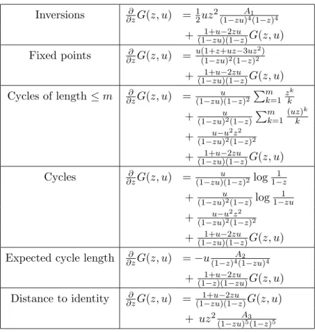
Using also the equations for R(z, v) and ˜R(z, v) of Section 2, we obtain first-order differential equations for G(z, u) resp. ˜G(z, u) with initial valuesG(0, u) = 0 resp. ˜G(0, u) = 0, that are given in Table 1.
Table 1: Differential equations for G(z, u) resp. ˜G(z, u).
Inversions ∂z∂G(z, u) = 12uz2 A1
(1−zu)4(1−z)4
+(11+−zuu−)(12zu−z)G(z, u) Fixed points ∂z∂G(z, u) = u(1(1+−zzu+)uz2(1−−3zuz)22)
+(11+−zuu−)(12zu−z)G(z, u) Cycles of length≤m ∂z∂G(z, u) = (1−zuu)(1−z)2
Pm
k=1z k
k
+(1−zu)u2(1−z) Pm
k=1
(uz)k
k
+(1−zuu−)u22(1z2−z)2 +(11+−zuu−)(12zu−z)G(z, u) Cycles ∂z∂G(z, u) = (1−zu)(1u −z)2 log1−1z
+(1−zu)u2(1−z)log1−1zu +(1−zuu−)u22(1z2−z)2
+(11+−zuu−)(12zu−z)G(z, u) Expected cycle length ∂z∂G(z, u) =−u A2
(1−z)4(1−zu)4
+(11+−zu)(1−2−zuzu)G(z, u) Distance to identity ∂z∂G(z, u) = (11+−zuu−)(12zu−z)G(z, u)
+ uz2 A3
(1−zu)5(1−z)5
The quantities A1, A2,A3 are defined asA1 = 1−3uz−3u2z+ 6u2z2 −u2z3 −u3z3 +u2, A2 = u3z6 −2u3z5 −2u2z5 + 2u3z4 + 3u2z4 + 2uz4−3u2z3 −3uz3 −u2z2+ 3uz2 −z2+uz +z−1 and A3 =u4z4+u2z4−4u3z3−4u2z3+ 12u2z2−4u2z−4uz+u2+ 1.
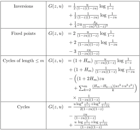
Solving these equations gives the expressions for G(z, u) resp. ˜
G(z, u), that are summarized in Table 2.
Table 2: Solutions forG(z, u) resp. ˜G(z, u).
Inversions G(z, u) = 12(1−z)(1u−zu)log1−1z +12(1−z)(11−zu)log1−1zu +14zu A4
(1−zu)3(1−z)3
Fixed points G(z, u) = 2 (1−zuu)(1−z)log1−1z + 2(1−zu1)(1−z)log1−1zu
−3 (1−zuzu)(1−z)
Cycles of length≤m G(z, u) = (1 +Hm)(1−zuu)(1−z)log1−1z
+ (1 +Hm) (1−zu1)(1−z)log1−1zu
−(1 + 2Hm)zu
+Pm
k=2
(Hm−Hk−1)(uzk+ukzk)
k
×(1−zu1)(1−z)
Cycles G(z, u) = ulog 2 1
1−z+log
2 1 1−zu
2(1−zu)(1−z)
−(1−zuzu)(1−z)
+ulog 1 1−z+log
1 1−zu
(1−zu)(1−z)
The abbreviations areA4 = 3z3u2+ 3z3u−2z2u2−12z2u−2z2+ 7zu+ 7z−4, A5 =−2z4u2+ 5z3u2+ 5z3u−2z2u2−12z2u−2z2+ 5zu+ 5z−2, A6 =u3z3+u2z3−6u2z2+ 3u2z+ 3uz−u2−1.
With the approach presented here that leads to explicit solutions, we can treat parameters that satisfy the general recursive structure
nan,j =Tn,j + j−1 X
k=1
an−k,j−k+ n
X
k=j+1 ak−1,j,
Expected cycle length G(z, u) = (1−z)(1u−zu)log1−1z +(1−z)(11−zu)log1−1zu +12zu A5
(1−zu)3(1−z)3
Distance to identity G(z, u) =−1
3 uz
3 A6
(1−zu)4(1−z)4
with toll functions Tn,j = f1(n) +f2(j) + f3(n−j), where fi(m)
are linear combinations of terms mpHm and mp with nonnegative
integersp. This recurrence with such “harmonic” toll functionsf1(n) (butf2(j) =f3(n−j) = 0) was studied in [10].
4.2 Quickselect with median-of-three pivoting
From the recurrence relations (19) we get the following third-order linear differential equations, where we use the abbreviations R0(z, v) := ∂z∂R(z, v), resp. ˜R0(z, v) := ∂z∂R(z, v).˜
• Inversions and distance to the identity permutation: ∂3
∂z3F(z, u, v) = 6u
2R0(zu, v) ∂
∂zF(z, u, v)
+ 6u2R0(zu, v)R0(z, v) + 6R0(z, v) ∂
∂zF(z, u, v). (22a)
• Fixed points and cycles: ∂3
∂z3F(z, u, v) = 6u
2vR0
(zu, v) ∂
∂zF(z, u, v) (22b) + 6u2vR0(zu, v)R0(z, v) + 6vR0(z, v) ∂
∂zF(z, u, v).
• Expected cycle length: ∂3
∂z3F(z, u, v) = 6u˜
2vR˜0(zu, v) ∂
∂zF˜(z, u, v) (22c) + 6u2vR˜0(zu, v) ˜R0(z, v) + 6vR˜0(z, v) ∂
∂zF˜(z, u, v). In order to get the expected value of our parameters, we differen-tiate the functions F(z, u, v) resp. ˜F(z, u, v) w. r. t. v and evaluate atv= 1. Here we define the functions
Φ(z, u) = ∂ ∂v
∂
∂zF(z, u, v)
v=1, resp. ˜Φ(z, u) = ∂ ∂v
∂
∂zF˜(z, u, v)
v=1 (23)
and obtain E(Qn,j) = n1[zn−1uj]Φ(z, u) for all parameters except
the expected cycle length, where we obtain E(Qn,j) = 1nE( ˜Qn,j) =
1
n2[zn−1uj] ˜Φ(z, u).
This leads to second-order linear differential equations for Φ(z, u) (resp. ˜Φ(z, u)), where the functions R0(z,1)
v=1 (resp. ˜R
0(z,1)
v=1) appearing are obtained by differentiating the equations of Section 2. These differential equations are given as Table 3. The initial values are given by Φ(0, u) = 0 and ∂z∂ Φ(z, u)|z=0 = 0 for the inversions and the distance to the identity permutation, by Φ(0, u) = u and
∂
∂zΦ(z, u)|z=0= 4u+4u
2 for fixed points and cycles, and by ˜Φ(0, u) = u and ∂z∂Φ(z, u)˜ |z=0= 4u+ 4u2 for the expected cycle length.
Table 3: Differential equations for Φ(z, u) resp. ˜Φ(z, u).
Inversions ∂z∂22Φ(z, u) =
3zu4(2+zu)(1−uz2)
(1−zu)6(1−z)2 +
6u2
(1−zu)2Φ(z, u) +(13−zuzu3)(2+4(1zu−z))2 +
3zu2(2+z)
(1−zu)2(1−z)4
+3(1zu−(2+zuz)2)(1(1−−zz2)6u) + 6
(1−z)2Φ(z, u) Fixed points ∂z∂22Φ(z, u) =
12u3(1−z2u)
(1−zu)4(1−z)2 + 6u
2
(1−zu)2Φ(z, u) +(1−zu18)2u(12−z)2 +
12u(1−z2u)
(1−zu)2(1−z)4
+(1−6z)2Φ(z, u) Cycles ∂z∂22Φ(z, u) =
12u3(1−z2u)
(1−zu)4(1−z)2
+(16−uzu3(1)4−(1z2−uz))2 log 1
1−zu
+(1−6uzu2)2Φ(z, u) +
18u2
(1−zu)2(1−z)2
+(1−zu6)u2(12 −z)2 log 1
1−zu
+(1−zu6)u2(12 −z)2 log 1
1−z+
12u(1−z2u)
(1−zu)2(1−z)4
+(1−6uzu(1)−2(1z2−u)z)4 log 1
1−z+
6
(1−z)2Φ(z, u)
To solve the differential equation ∂2
∂z2Φ(z, u)−6
1 (1−z)2 +
u2 (1−zu)2
Φ(z, u) =g(z, u) with different g(z, u)’s according to the parameter under considera-tion, we can transform it into a hypergeometric differential equation
Expected ∂z∂22Φ(z, u)˜ =
6u2(u−z2u2)
(1−zu)4(1−z)2
cycle length +6u2(1(1+2−zuzu)6)((1u−−zz)22u2)+ 6u 2
(1−zu)2Φ(z, u)˜ +(1−zu6)u22(1−z)2 +
6u2(1+2zu)
(1−zu)4(1−z)2
+(1−6uzu2(1+2)2(1−z)z)4 +
6(u−z2u2)
(1−zu)2(1−z)4
+6(1+2(1−zz)6)((1u−−zuz2u)22)+(1−6z)2Φ(z, u)˜
Distance ∂z∂22Φ(z, u) =
12zu4(1+zu)(1−z2u)
(1−zu)7(1−z)2 +
6u2
(1−zu)2Φ(z, u) to identity +(112−zuzu4)(1+5(1−zuz))2 +
12zu2(1+z)
(1−zu)2(1−z)5
+12(1zu−(1+zu)z2)(1(1−−zz)27u) + 6
(1−z)2Φ(z, u)
t(1−t)∂ 2
∂t2G(t, u)−4(1−2t) ∂
∂tG(t, u)−8G(t, u) = t
3(1−t)3(1−u)6
u4 g 1 +
1−u
u t, u
. There we used the substitutions
Φ(z, u) = 1
(1−z)2(1−zu)2E(z, u),
z= 1 +1−uutand G(t, u) =E 1 +1−uut, u. This procedure was also used in [6].
The corresponding homogeneous differential equation has the so-lution
Ghom(t, u) =k1(u)(1−2t) +k2(u)t5
1−2t+10 7 t
2− 5
14t
3.
Solving the inhomogeneous differential equations by variation of the constants, we obtain after back substituting the solutions of the func-tions Φ(z, u) resp. ˜Φ(z, u).1 Since these solutions are very lengthy, we refrain from printing them here. We only give the structure of Φ(z) in the instance of cycles (the structure is very similar for the other parameters):
Φ(z) = P1(z, u)
(1−z)2(1−u)7(1−uz)2 Z z
t=0
log1−1t 1−utdt 1
This technique is described in more detail in [9]. The paper [10] is also of relevance here.
+ P2(z, u)
(1−z)2(1−u)7(1−uz)2 log
2 1
1−z (24)
+ P3(z, u)
(1−z)2(1−u)7(1−uz)2 log 1 1−z + P4(z, u)
(1−z)2(1−u)7(1−uz)2 log
2 1
1−uz + P5(z, u)
(1−z)2(1−u)7(1−uz)2 log 1 1−uz + P6(z, u)
(1−u)7(1−uz)2 log 1 1−zlog
1 1−uz + P7(z, u)
(1−z)2(1−u)7(1−uz)2,
with certain polynomialsPi(z, u) inzand ufor 1≤i≤7. Of course,
these solutions are obtained with assistance of a computer algebra system.
5
Extracting coefficients
To obtain the desired expectations E(Qn,j) of the parameters
con-sidered, we have to extract coefficients from the generating functions computed in Section 4. We will use the following identities.
[znuj] 1
(1−z)m+1(1−uz)m+1 =
m+j m
n−j+m m
,
for 0≤j≤nandn≥0,
[znuj] u
(1−uz)(1−z)log 1
1−z =Hn+1−j and
[znuj] u
(1−uz)(1−z)log
2 1
1−z =H 2
n+1−j−H
(2)
n+1−j,
for 1≤j ≤nandn≥1, [znuj] 1
(1−uz)(1−z)log 1
1−uz =Hj and
[znuj] 1
(1−uz)(1−z)log
2 1
1−uz =H 2
j −H
(2)
j ,
for 1≤j≤nandn≥1.
5.1 Ordinary quickselect
5.1.1 Explicit results
Extracting coefficients fromG(z, u) resp. ˜G(z, u) as given in Table 2, we obtain the following explicit results forE(Qn,j).
• Inversions:
E(Qn,j) =
1
8(n+ 1−j)(n−4−j) + 1
8j(j−5) + 1
2Hn+1−j+ 1 2Hj. (25a)
• Fixed points:
E(Qn,j) = 2Hn+1−j+ 2Hj −3. (25b)
• Cycles of length up to mwhen m−1< j < n−m+ 2:
E(Qn,j) = (1 +Hm)(Hn+1−j+Hj)−
1 +Hm2 +Hm(2). (25c)
• Cycles:
E(Qn,j) =
1 2H
2
n+1−j−
1 2H
(2)
n+1−j+
1 2H
2
j−
1 2H
(2)
j −1+Hn+1−j+Hj.
(25d)
• Expected cycle length:
E(Qn,j) =
1 n
1
4(n+1−j)(n−j)+ 1
4j(j−1)−1+Hn+1−j+Hj
. (25e)
• Distance to the identity permutation:
E(Qn,j) =
1 18 n
3−n
−1
6(n−1)j(n+ 1−j). (25f) 5.1.2 Grand averages
The grand averages are defined by En:=E
1 n
n
X
j=1 Qn,j
. (26)
They can be obtained by En=
1 n[z
n]G(z,1) (27a)
for all parameters except the expected cycle length, where we have En=
1 n2[z
n] ˜G(z,1). (27b)
The required generating functions are given in Table 4. Table 4: The functionsG(z,1) resp. ˜G(z,1).
Inversions G(z,1) = (1−1z)2 log1−1z +123z 2−2z
(1−z)4
Fixed points G(z,1) = (1−4z)2 log 1
1−z −
3z
(1−z)2
Cycles up to lengthm G(z,1) = 2(1 +Hm)(1−1z)2log1−1z
−(1 + 2Hm)z
+ 2Pm
k=2 1
k(Hm−Hk−1)z k
× 1
(1−z)2
Cycles G(z,1) = (1−1z)2 log
2 1
1−z−
z
(1−z)2
+ 2(1−1z)2log1−1z Expected cycle length G(z,˜ 1) = 2(1−1z)2 log1−1z+
−z(z2−3z+1)
(1−z)4
Distance to identity G(z,1) = 23(1−z3z)5
Extracting coefficients leads then to the following explicit and asymptotic results for the grand averagesEn.
• Inversions: En=
1 + 1
n
Hn+
n2−6n−19
12 ∼
n2
12. (28a)
• Fixed points:
En= 4
1 + 1
n
Hn−7∼4 logn. (28b)
• Cycles up to lengthm: En= 2(1 +Hm)Hn
1 + 1
n
−2(1 +Hm)−
1 + 1
n
Hm2
−1 + 1 n
Hm(2)−1 + 2m
n forn > m−2 (28c)
∼2(1 +Hm).
• Cycles: En=
Hn2−Hn(2) 1 + 1 n
+ 2
nHn−1∼log
2n. (28d)
• Expected cycle length: En=
2 n
1 + 1 n
Hn+
1 6n
1−19
n2
∼ n
6. (28e)
• Distance to the identity permutation:
En=
1
36(n+ 1)(n−1)(n−2)∼ n3
36. (28f)
5.2 Quickselect with median-of-three pivoting
5.2.1 Explicit results
By extracting coefficients from Φ(z, u) resp. ˜Φ(z, u) as computed in Subsection 4.2, one can obtain explicit results for E(Qn,j) also for
quickselect with median-of-three pivoting. For the sake of complete-ness, we give these lengthy formulæ in the appendix.
They are obtained by using formulæ (3) and (4) under heavy usage of a computer algebra system to simplify and manipulate the resulting expressions. As an example, we consider the instance of cycles, where the formula for Φ(z) is given as (24), in a bit more detail. Picking for instance the summand
sn,j = [znuj]
P2(z, u)
(1−z)2(1−u)7(1−uz)2log
2 1
1−z,
where P2(z, u) is a polynomial in z and u, it is apparent that it is sufficient to compute
tn,j = [znuj]
1
(1−z)2(1−u)7(1−uz)2log
2 1
1−z,
since the required coefficient sn,j is obtained by a linear
combina-tion of such shifted expressions: sn,j =Pm≤M,l≤Lαm,ltn−m,j−l, with
certain bounds L,M and coefficientsαm,l.
Using (3), we obtain immediately [znuj] 1
(1−z)2(1−u)7(1−uz)2 log
2 1
1−z =
n
X
k=n−j
(n−k+ 1)
j−n+k+ 6 6
(k+ 1)× × (Hk+1−1)2−(H
(2)
k+1−1)
.
To obtain a closed formula for this expression, one requires closed forms for sums Pn
k=1kpHk2,
Pn
k=1kpHk and
Pn
k=1kpH (2)
k for
non-negative integersp≤8. Such identities like
n
X
k=1
Hk2 = (n+ 1)Hn2+1−(2n+ 3)Hn+1+ 2(n+ 1),
can be computed by standard manipulations of harmonic numbers and are also generated “automatically” by computer algebra systems like MAPLE.
The given explicit expressions in the appendix were checked by the authors for a lot of “small” numbers j andn.
5.2.2 Grand averages
The grand averagesEn can now be obtained by
En=
1 n2[z
n−1]Φ(z,1) (29a)
for all parameters except the expected cycle length, where we have En=
1 n3[z
n−1] ˜Φ(z,1). (29b)
The explicit and asymptotic results obtained here are summarized in the following.
• Inversions: En=
6 7+
6 7n
Hn+
1 12n
2−1
2n− 793 588+
9 98n ∼
n2
12 forn≥6, (30a) E1= 0, E2= 0, E3= 0, E4=
1
4, E5 = 3 5.
• Fixed points: En=
24 7 +
24 7n
Hn−
38 49n−
255 49 ∼
24
7 logn forn≥6, (30b) E1 = 1, E2 = 2, E3 = 3, E4 =
7 2, E5=
101 25 .
• Cycles: En=
6 7 +
6 7n
Hn2+30 49 +
114 49n
Hn−
6 7n+
6 7
Hn(2)
− 65
343n− 618 343∼
6 7log
2n forn≥6, (30c)
E1 = 1, E2 = 2, E3 = 3, E4 = 15
4 , E5= 112
25 .
• Expected cycle length: En=
1 6n−
793 294n+
9 49
1 n2 +
12 7
1 n2 +
1 n
Hn∼
n
6 forn≥6, (30d) E1 = 1, E2 = 1, E3 = 1, E4 =
9
8, E5 = 31 25.
• Distance to the identity permutation: En=
(n+ 1)(14n3−49n2+ 14n+ 36)
525n ∼
2n3
75 forn≥6, (30e) E1 = 0, E2 = 0, E3 = 0, E4 =
1
2, E5 = 36 25.
6
Variances
6.1 Explicit results
In principle, it is also possible to obtain explicit expressions for higher moments of Qn,j from equations (20), in particular for the variance
V(Qn,j). It turns out that the explicit expressions that we obtain for
the second factorial momentE Qn,j(Qn,j −1)
for ordinary quickse-lect are already of daunting complexity. Defining
H(z, u) = ∂2
∂v2F(z, u, v)
v=1
resp. ˜H(z, u) = ∂2
∂v2F˜(z, u, v)
v=1 , (31)
the second factorial moments are given by E Qn,j(Qn,j−1)
= [znuj]H(z, u) for all parameters except the expected cycle length, where we obtain E Q˜n,j( ˜Qn,j −1)
= [znuj] ˜H(z, u). For the sake of completeness, we give these findings in the appendix. We refrain from doing such calculations for the more complicated instance of median-of-three partition.
6.2 The variance of the mean
Of particular interest is the variance of the mean
Vn:=V
1 n
n
X
j=1 Qn,j
(32)
for our parameters. This quantity can be obtained by evaluating at u= 1 at the level of generating functions and extracting coefficients. One gets
Vn=
1 n2[z
n]H(z,1) + 1
nEn−E 2
n (33a)
for all parameters considered except the expected cycle length, where we get
Vn=
1 n4[z
n] ˜H(z,1) + 1
n2En−E 2
n.
The appearing En are the grand averages as computed in
Subsec-tion 5.1.2.
Next we summarize the obtained explicit and asymptotic results.
• Inversions: Vn=
n4 720+
5n3 432 −
11n2 216 +
247n 432 +
4607 2160−
1 n+
1 n2
Hn2
+
−n
6 − 1 3 +
11 6n
Hn−
1 + 1
n
Hn(2), n≥1
∼ n
4
720. (34a)
• Fixed points: Vn=−
16 +16 n
Hn(2)−16
n + 16 n2
Hn2+ 58
n + 10
Hn
− 19
3n+ 5
3, forn≥2, V1 = 0. (34b)
• Cycles: Vn=
−4− 2
n+ 2 n2
Hn2Hn(2)+2 3−
4 n2 +
2 3n
Hn3
− 1
n2 + 1 n
Hn4+− 1
n2 + 2 + 1 n
Hn(2)2
+ 5
n + 5− 4 n2
Hn2+
4 3 +
28 3n
Hn(3)+
−8− 1
6n
Hn
−5 +5 n
Hn(2)−6 +6 n
Hn(4)+
4
n2 −2− 10
n
HnHn(2)
+8 n + 8
HnHn(3)+ 18, forn≥1 (34c)
∼ 2
3log
3n.
• Expected cycle length: Vn=
1 720
7n4+ 25n3−185n2+ 1895n+ 6898
n2 −
4(n+ 1) n4 H
2
n
−4(n+ 1)
n3 H (2)
n −
2 3
(n+ 5)(n−2)
n3 Hn, forn≥1 (34d) ∼ 7n
2 720.
• Distance to the identity permutation: Vn=
(n−1)(n−2)(n+ 1)(145n3+ 836n2+ 53n−398)
226800 ,
forn≥1
∼ 29n 6
45360. (34e)
7
Conclusion
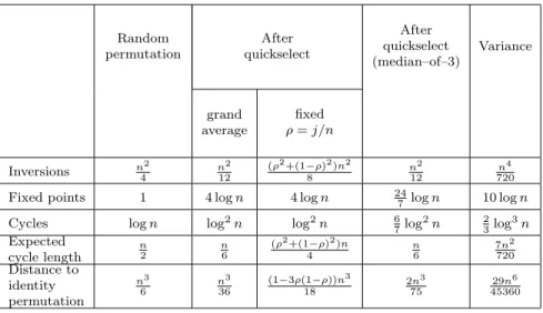
In Table 5 we collect our basic findings. Note for instance that the number of cycles is increasing, since we are “closer” to the identity permutation, which has the most number of cycles.
At first glance it might seem surprising that the parameters “num-ber of fixed points” and “num“num-ber of cycles” are smaller after the median-of-three algorithm than after the ordinary quickselect algo-rithm, which means that for these statistics the permutations are
Table 5: Averages and variances with/without one round of quickse-lect (leading term only).
Random permutation
After quickselect
After quickselect (median–of–3)
Variance
grand average
fixed
ρ=j/n
Inversions n42 n122 (ρ2+(1−8ρ)2)n2 n122 720n4
Fixed points 1 4 logn 4 logn 247 logn 10 logn
Cycles logn log2n log2n 67log2n 23log3n
Expected cycle length
n
2
n
6
(ρ2+(1−ρ)2)n
4
n
6
7n2
720 Distance to
identity permutation
n3
6
n3
36
(1−3ρ(1−ρ))n3 18
2n3
75
29n6
45360
on average more disordered in the median-of-three case. The reason for this is that with median-of-three partition the number of recursive calls in the algorithm decreases and thus the requested element can be found “faster.” Because every recursive call places one pivot element in the correct position and on average in every segment between the pivots we have one additional fixed point (these segments are random permutations), one expects that the average number of fixed points will asymptotically behave like twice the average number of recursive calls in Quickselect, a parameter that was studied in [6]. With the heuristic that for largenalmost no pivots are neighbors, we get that asymptotically the number of fixed points is twice the number of piv-ots (or recursive calls). On average we make in the median-of-three case asymptotically 1/7 fewer recursive calls and thus we have about 1/7 fewer fixed points.
8
Appendix
8.1 Explicit results for median-of-three pivoting
We use here the abbreviationEn,j :=E(Qn,j).
• Inversions:
En,j=−
6 35Hn(3n
2−6jn−3n+ 4−6j+ 6j2) + 9 35Hj(2j
2−6j+ 5)
+ 9
35Hn+1−j(2n 2−
2n−4jn+ 2j2+ 2j+ 1)− 6
7j
− 6
7(n+ 1−j) + 3 28n 2 +18 35jn −167
140n+ 814 245
− 921
2450j 2−153
70j
− 3
35
48j−25−36j2+ 3j3
n +
3 35
(j2−2j+ 10)(j−1)2
n(n−1) + 1
175
(j−1)(j−2)(2j−3)(3j2−9j+ 50)
n(n−1)(n−2) + 3
175
(j−1)(j−3)(j2−4j+ 25)(j−2)2
n(n−1)(n−2)(n−3)
− 3
245
(j−1)(j−2)(j−3)(j−4)(2j−5)(j2−5j+ 35)
n(n−1)(n−2)(n−3)(n−4) + 1
490
(j−1)(j−2)(j−4)(j−5)(3j2−18j+ 140)(j−3)2
n(n−1)(n−2)(n−3)(n−4)(n−5) for 5
≤j≤n−4,
En,4=−87
35Hn+ 1 4900
525n5−4900n4−131843n2+ 48556n3+ 104042n−13440
n(n−1)(n−2) forn≥8,
E4,4=1 4, E5,4=
13 20, E6,4=
17 20, E7,4=
13 10,
En,3=− 3 7Hn+
1 980
105n4−770n3−2090n+ 2755n2−588
n(n−1) forn≥7, E3,3= 0, E4,3=
1 4, E5,3=
2 5, E6,3=
17 20,
En,2= 3 28n
2−19 28n−
1 175+
3
5Hnforn≥6, E2,2= 0, E3,2= 0, E4,2= 1 4, E5,2=
13 20,
En,1= 3 28n
2−19 28n
− 1
175+ 3 5Hnforn
≥5, E1,1= 0, E2,1= 0, E3,1= 0, E4,1= 1 4.
• Fixed points:
En,j=
48 35Hn+
36 35Hj+
36
35Hn+1−j+ 24 35j+
24 35(n+ 1−j)
−583
175+ 12 35
3j−5
n −
24 35
(j−1)2
n(n−1)− 8 35
(j−1)(j−2)(2j−3)
n(n−2)(n−1) − 12 35
(j−1)(j−3)(j−2)2
n(n−2)(n−1)(n−3) +12
35
(2j−5)(j−1)(j−2)(j−3)(j−4)
n(n−2)(n−1)(n−3)(n−4) − 8 35
(j−5)(j−1)(j−2)(j−4)(j−3)2
n(n−2)(n−1)(n−3)(n−4)(n−5) for 5≤j≤n−4,
En,4=12 5Hn−
1 175
−537n2+ 179n3+ 1618n−1680
n(n−2)(n−1) forn≥8,
E4,4= 7
2, E5,4= 4, E6,4= 23
5, E7,4= 5,
En,3= 12
5Hn− 1 175
209n2−209n+ 420
n(n−1) forn≥7, E3,3= 3, E4,3= 7 2, E5,3=
21 5, E6,3=
23 5,
En,2=− 37 25+
12
5Hnforn≥6, E2,2= 2, E3,2= 3, E4,2= 7
2, E5,2= 4,
En,1=− 37 25+
12 5Hnforn
≥5, E1,1= 1, E2,1= 2, E3,1= 3, E4,1= 7 2.
• Cycles:
En,j=
12 35HnHj+
12
35HnHn+1−j+ 34
35− 12 35j−
12 35(n+ 1−j)
Hn+
9 35H 2 j+ 9 35H 2
n+1−j
−12
35HjHn+1−j+ 12
35j+
12 35(n+ 1−j)+
103 175 −12 35 j n − 6 35
j(j−1)
nn−1
− 4
35
j(j−1)j−2
n(n−1)(n−2)
− 3
35
j(j−1)(j−2)(j−3)
n(n−1)(n−2)(n−3)+ 6 35
j(j−1)(j−2)(j−3)(j−4)
n(n−1)(n−2)(n−3)(n−4)
− 2
35
j(j−1)(j−2)(j−3)(j−4)(j−5)
n(n−1)(n−2)(n−3)(n−4)(n−5)
Hj
+12 35j+
12 35(n+ 1−j)−
2 175+
6 7
j−1
n −
6 35
(j−1)(j−2)
n(n−1) − 4 35
(j−1)(j−2)(j−3)
n(n−1)(n−2)
− 3
35
(j−1)(j−2)(j−3)(j−4)
n(n−1)(n−2)(n−3) + 6 35
(j−1)(j−2)(j−3)(j−4)(j−5)
n(n−1)(n−2)(n−3)(n−4)
− 2
35
(j−1)(j−2)(j−3)(j−4)(j−5)(j−6)
n(n−1)(n−2)(n−3)(n−4)(n−5)
Hn+1−j
−3 5H (2) j − 3 5H (2)
n+1−j+
1 35
17n+ 5 (n+ 1)(n+ 1−j)+
1 35
17n+ 5 (n+ 1)j−
6221 5250−
1 175
2j+ 23
n
− 1
35
(3j−7)(j−1)
n(n−1) + 1 105
(8j−9)(j−1)(j−2)
n(n−1)(n−2) + 1 35
(9j−28)(j−1)(j−2)(j−3)
n(n−1)(n−2)(n−3)
− 2
175
(31j−90)(j−1)(j−2)(j−3)(j−4)
n(n−1)(n−2)(n−3)(n−4) + 62
525
(j−1)(j−2)(j−3)2(j−4)(j−5)
n(n−1)(n−2)(n−3)(n−4)(n−5)for 5≤j≤n−4,
En,4= 3 5H 2 n+ 6 25
4n3−12n2−7n+ 20
n(n−1)(n−2) Hn− 3 5H (2) n + 3 3500
53760n+ 701n6+ 4353n4−11200 + 24348n3−66356n2−4206n5
n2(n−1)2(n−2)2 forn≥8,
E4,4= 15
4, E5,4= 89 20, E6,4=
21 4, E7,4=
59 10,
En,3= 3 5H 2 n+ 6 25
4n2−4n−5
n(n−1) Hn
−3 5H (2) n + 2 875
−525−282n3−454n2+ 141n4+ 1645n n2(n−1)2
forn≥7, E3,3= 3, E4,3= 15
4, E5,3= 23
5, E6,3= 21
4,
En,2=3 5H
2
n+
24 25Hn−
3 5H
(2)
n +
1
125 forn≥6, E2,2= 2, E3,2= 3, E4,2= 15
4, E5,2= 89 20,
En,1=3 5H
2
n+
24 25Hn−
3 5H
(2)
n +
1
125 forn≥5, E1,1= 1, E2,1= 2, E3,1= 3, E4,1= 15
4.
• Expected cycle length:
En,j=
18 35
2j2−6j+ 5
n Hj+
18 35
2n2−4jn−2n+ 2j2+ 2j+ 1
n Hn+1−j
−12
35
3n2−6jn−3n+ 6j2−6j+ 4
n Hn−
12 7 1 jn− 12 7 1 (n+ 1−j)n+
3 14n+
36 35j
−97
70+ 1628 245n−
921 1225 j2 n − 153 35 j n− 6 35
48j−25−36j2+ 3j3 n2 + 6
35
(j2−2j+ 10)(j−1)2
n2(n−1) + 2 175
(j−1)(j−2)(2j−3)(3j2−9j+ 50)
n2(n−1)(n−2) + 6
175
(j−1)(j−3)(j2−4j+ 25)(j−2)2
n2(n−1)(n−2)(n−3)
− 6
245
(j−1)(j−2)(j−3)(j−4)(2j−5)(j2−5j+ 35)
n2(n−1)(n−2)(n−3)(n−4)
+ 1 245
(j−1)(j−2)(j−4)(j−5)(3j2−18j+ 140)(j−3)2
n2(n−1)(n−2)(n−3)(n−4)(n−5) for 5≤j≤n−4,
En,4=− 174 35 Hn n + 1 2450
525n5−2450n4+ 41206n3−126943n2+ 104042n−13440
n2(n−1)(n−2) forn≥8,
E4,4= 9 8, E5,4=
63 50, E6,4=
77 60, E7,4=
48 35,
En,3=− 6 7 Hn n + 1 490
105n4−280n3+ 2265n2−2090n−588
n2(n−1) forn
≥7,
E3,3= 1, E4,3= 9 8, E5,3=
29 25, E6,3=
77 60,
En,2= 6 5 Hn n + 3n 14− 5 14− 2
175nforn≥6, E2,2= 1, E3,2= 1, E4,2=
9 8, E5,2=
63 50,
En,1= 6 5 Hn n + 3n 14− 5 14− 2
175nforn≥5, E1,1= 1, E2,1= 1, E3,1= 1, E4,1=
9 8.
• Distance to the identity permutation:
En,j=
6 35Hn(7n
3−21jn2−9n2+ 21j2n+ 2n+ 18jn−18−39j2+ 39j)
− 6
35Hj(j−1)(j−2)(7j−9)− 6
35Hn+1−j(7n−2−7j)(n−j)(n−1−j) + 1
24n 3−6
5jn 2
+143 140n
2−3419 840n+
9 4j
2
n+279 140jn
−255
28j+ 70743 4900 −21 10j 3 + 57 196j 2 −108
35j−
108 35(n+ 1−j)+
3 140
49j4−218j3+ 803j2−850j+ 360
n
+ 6 35
(5j2−10j+ 18)(j−1)2
n(n−1) + 6 35
(j−1)(j−2)(2j−3)(j2−3j+ 6)
n(n−1)(n−2) + 6
35
(j−1)(j−3)(j2−4j+ 9)(j−2)2
n(n−1)(n−2)(n−3)
− 6
245
(j−1)(j−2)(j−3)(j−4)(2j−5)(5j2−25j+ 63)
n(n−1)(n−2)(n−3)(n−4) + 3
245
(j−1)(j−2)(j−4)(j−5)(5j2−30j+ 84)(j−3)2
n(n−1)(n−2)(n−3)(n−4)(n−5) for 5≤j≤n−4,
En,4= 684 35Hn+
1 29400
1225n4−5250n3−127225n2−711282n+ 302400
n forn≥8,
E4,4= 1 2, E5,4=
8
5, E6,4= 2, E7,4= 16
5,
En,3= 1 24n
3−5 28n
2−223 168n+
144 35Hn−
13177
4900 forn≥7, E3,3= 0, E4,3= 1 2, E5,3=
4
5, E6,3= 2,
En,2=− 5 28n 2 + 1 24n 3 + 29 168n − 1
140 forn
≥6, E2,2= 0, E3,2= 0, E4,2= 1 2, E5,2=
8 5,
En,1=−5
28n 2 + 1 24n 3 + 29
168n− 1
140 forn≥5, E1,1= 0, E2,1= 0, E3,1= 0, E4,1= 1 2.
Due to the symmetry En,j = En+1−j,j, this parameter is fully
described by the above values.
8.2 Explicit expressions for the second factorial mo-ments for ordinary quickselect
We obtain the following results for the second factorial moments Mn,j(2):=E Qn,j(Qn,j −1)
.
• Inversions:
Mn,j(2)=−1
4H (2) j − 1 4H (2)
n+1−j
− 1
24
Hn(n+ 1)(n3j−4n2j2+ 3n2j+ 6j3n−8j2n−10jn+ 9j2−3j4−12 + 6j3−12j)
j(n+ 1−j) +1 4H 2 j+ 1 4H 2
n+1−j+
1
2Hn+1−jHj + 1
24
Hj
j(n+ 1−j)(3n 3
j−12n2j−9n2j2+ 12j3n−4j2n+j4n−12n−43jn+ 15j2−j5
−28j−5j4+ 19j3−12) + 1
24
Hn+1−j
j(n+ 1−j)(n
4j+ 7n3j−4n3j2−21n2j2−13n2j+ 6n2j3−12n−53jn+ 5j2n
+ 24j3n−4j4n−10j4−34j+ 32j2+ 11j3+j5−12) + 1
3456 1
j(n+ 1−j)(1626j 4
+ 702j5−4422j3−4296j2+ 6624j−234j6+ 1728 + 702j5n
+ 63jn5+ 9382jn−805n3j+ 3783n2j2+ 2191n2j−5094j3n−834j4n+ 2468j2n
−175n4j+ 304n3j2−954j4n2+ 66n2j3−315n4j2+ 738n3j3) forn≥j≥1.
• Fixed points:
Mn,j(2)=−4H(2)j −4Hn(2)+1−j+ 8 Hn(n+ 1) (n+ 1−j)j+ 4H
2
j+ 4H
2
n+1−j+ 8Hn+1−jHj
−Hj(−9j
2+ 9jn+ 9j+ 8n+ 8) (n+ 1−j)j −
Hn+1−j(−9j2+ 9jn+ 9j+ 8n+ 8)
(n+ 1−j)j
+1 3
118j+ 23n2j2−46j3+ 47n2j−46j3n−j2n+ 23j4+ 60n−95j2+ 72 + 165jn+ 12n2 j(n+ 2−j)(j+ 1)(n+ 1−j)
forn−1≥j≥2, Mn,(2)1= 4Hn2−4H(2)n −Hn+4
n−
5 2 forn≥2, M(2)1,1= 0.
• Cycles:
Mn,j(2)= ( 2 (n+ 1−j)2−
2
n+ 1−j
−2Hn+1−j
n+ 1−j)
j
X
k=1
Hn−j+k
k + (
2
j2− 2
j
−2Hj
j )
n+1−j
X
k=1
Hk+j−1
k
+ 2Hn+1−jHn(3)+1−j+ 2HjHj(3)−4HjHj(2)−4Hn+1−jHn(2)+1−j−
3 2H
(4)
n+1−j−
3 2H (4) j +8 3H (3)
n+1−j+
8 3H
(3)
j +
3 4(H
(2)
j )
2 +3
4(H (2)
n+1−j)
2−3 2H 2 jH (2) j − 3 2H 2
n+1−jH
(2)
n+1−j
+1 4H 4 j+ 1 4H 4
n+1−j+
4 3H 3 j+ 4 3H 3
n+1−j+
1 2H
2
jH2n+1−j+
1 2H
(2)
j H
(2)
n+1−j −1
2H 2
jH
(2)
n+1−j−
1 2H
2
n+1−jH
(2)
j + (
1
j−1)HjH
(2)
n+1−j+ (
1
n+ 1−j−1)Hn+1−jH
(2)
j
+ (−1 +1
j
− 1
j2)H (2)
n+1−j+ (−1 +
1
n+ 1−j
− 1
(n+ 1−j)2)H (2)
j
+ (1−1
j)HjH
2
n+1−j+ (1−
1
n+ 1−j)Hn+1−jH
2
j
+ (−2
j2− 2
j+
1 (n+ 1−j)2−
1
n+ 1−j+ 1)H
2
j
+ (− 2
(n+ 1−j)2− 2
n+ 1−j+
1
j2− 1
j+ 1)H
2
n+1−j
+ (−2− 2(2n+ 1)
(n+ 1)(n+ 1−j)−
2
(n+ 1−j)2(n+ 1)+ 2 (n+ 1−j)3−
2(2n+ 1) (n+ 1)j
+ 2 (n+ 1)j2 +
2
j3)Hj + (−2− 2(2n+ 1)
(n+ 1)(n+ 1−j)+
2
(n+ 1−j)2(n+ 1)+ 2 (n+ 1−j)3−
2(2n+ 1) (n+ 1)j
− 2
(n+ 1)j2+ 2
j3)Hn+1−j + (2− 2n
(n+ 1)(n+ 1−j)− 2 (n+ 1−j)2−
2n
(n+ 1)j−
2
j2)HjHn+1−j + (2
j2+ 2
j−
2 (n+ 1−j)2+
2
n+ 1−j)HnHj
+ ( 2 (n+ 1−j)2 +
2
n+ 1−j−
2
j2+ 2
j)HnHn+1−j
+ (2
j+
2
n+ 1−j)HnHjHn+1−j+ (−
2
j3+ 4
j−
2 (n+ 1−j)3+
4
n+ 1−j)Hn
−2(2n−1)
(n+ 1)j −
2(2n−1) (n+ 1)(n+ 1−j)−
2 (n+ 1)j3−
2
(n+ 1)(n+ 1−j)3+ 12 forn≥j≥1.
• Expected cycle length:
Mn,j(2)=H 2
j
n2 +
H2n+1−j n2 −
Hj(2) n2 −
Hn(2)+1−j n2 + 2
HjHn+1−j
n2
−(1 6
n3−3jn2+ 3n2+ 3j2n−6jn−10n+ 3j2−3j−12
n2 −
2
jn2− 2
n2(n+ 1−j))Hn
+ (1 6
3n2−6jn−9n+j3+ 6j2−13j−18
n2 −
2
jn2− 2
n2(n+ 1−j))Hj + (1
6
n3−3jn2+ 6n2+ 3j2n−12jn−13n−j3+ 9j2−2j−24
n2
− 2
jn2− 2
n2(n+ 1−j))Hn+1−j + 1
72n2(6n
4−24jn3−2n3+ 45j2n2−9jn2−72n2−42j3n+ 27j2n+ 147jn+ 68n+ 21j4
−42j3−111j2+ 132j+ 432) + 2
jn2(n+ 1)+
2
n2(n+ 1−j)(n+ 1)forn≥j≥1.
• Distance to the identity permutation:
Mn,j(2)= 2
45Hn(n+ 1)(n 4−
5n3j+ 4n3+ 10n2j2+n2−15n2j+ 20j2n−10j3n−6n+ 10j−5j2
+ 5j4−10j3)− 2
45jHj(j−1)(j−2)(j+ 2)(j+ 1)
− 2
45Hn+1−j(n+ 1−j)(n−j)(n−1−j)(n+ 3−j)(n+ 2−j) +31n
6 6480
−n
5(−27 + 62j) 2160 +
n4(343 + 465j2−693j) 6480
−n
3(2588j+ 580j3−1986j2−687) 6480
+n
2(202 + 345j4−2466j3+ 5562j2−2349j)
6480 −
n(4628j3−1053j4+ 66j5−236j+ 1344−3909j2) 6480
+ 1
3240j(j−1)(11j
4−22j3+ 691j2−680j−252) forn≥j≥1.
References
[1] Comtet, L. (1974), Advanced Combinatorics. D. Reidel Publish-ing Company.
[2] Graham, R. L., Knuth, D. E., and Patashnik, O. (1994), Con-crete Mathematics. Second Edition, Reading, Massachussetts: Addison-Wesley.
[3] Greene, D. H. and Knuth. D. E. (1982), Mathematics for the Analysis of Algorithms. Second Edition, Berlin: Birkh¨auser. [4] Hoare, C. A. R. (1961), Find (Algorithm 65). Communications of
the ACM, 4, 321–322.
[5] Hoare, C. A. R. (1962), Quicksort. Computer Journal, 5, 10–15. [6] Kirschenhofer, P., Mart´ınez, C., and Prodinger, H. (1997),
Anal-ysis of Hoare’s Find algorithm with median–of–three partition. Random Structures and Algorithms, 10, 143–156.
[7] Knuth, D. E. (1998), The Art of Computer Programming. Vol-ume 3: Sorting and Searching, 2nd ed. Reading, Massachussetts: Addison-Wesley.
[8] Mart´ınez, C., Panholzer, A., and Prodinger, H. (1998), Descen-dants and ascenDescen-dants in random search trees. Electronic Journal of Combinatorics,5, R20.
[9] Panholzer, A. (1997), Untersuchungen zur durchschnittlichen Gestalt gewisser Baumfamilien (Mit besonderer Ber¨ucksichtigung von Anwendungen in der Informatik). Ph. D. Thesis, TU Vienna, 219 pages.
[10] Panholzer, A. and Prodinger, H. (2002), Binary search tree re-cursions with harmonic toll functions. Journal of Computational and Applied Mathematics, 142, 211–225.
[11] Sedgewick, R. and Flajolet, P. (1996), An Introduction to the Analysis of Algorithms. Reading, Massachussetts: Addison-Wesley.