Vol. 13, No. 1, pp 43-56
Analysis of Dependency Structure of Default
Processes Based on Bayesian Copula
Mohammad Seidpisheh1,2, Armin Pourkhanali3, Karim Norouzipour3, Adel Mohammadpour1
1Department of Statistics, Faculty of Mathematics and Computer Science,
Amirkabir University of Technology, Tehran, Iran.
2Department of Statistics, Allameh Tabataba’i University, Tehran, Iran. 3Department of Mathematics, Institute for Advanced Studies in Basic Sciences
(IASBS), Zanjan, Iran.
Abstract. One of the main problems in credit risk management is the correlated default. In large portfolios, computing the default depen-dencies among issuers is an essential part in quantifying the portfolio’s credit. The most important problems related to credit risk management are understanding the complex dependence structure of the associated variables and lacking the data. This paper aims at introducing a new methodology for credit risk management based on Bayesian copulas. In this paper, the focus is specifically on a new method of simulating the joint distribution of default risk. This methodology joins the use of cop-ulas and Bayesian models. Using copcop-ulas, the joint multivariate prob-ability distribution of a random vector can be separated into individ-ual components characterized by marginal distributions. The model is based on a jump diffusion process for the intensities. Another important problem in credit risk management is the lack of data, which influences the parameter estimation. Considering this drawback, the employment of Bayesian methods and simulation tools could be a natural solution to the problem. This suggests the use of Bayesian models, computed
Mohammad Seidpisheh(m84 [email protected]), Armin Pourkhanali ([email protected]), Karim Norouzipour([email protected]), Adel Mohammadpour( )([email protected])
Received: December 2012; Accepted: August 2013
via simulation methods and in particular, Markov chain Monte Carlo. Bayesian methods in Student’s t copula are efficient enough for heavy tail distribution. Moreover, our main outcome is that the application of Bayesian methodology causes a reduction of measure while that copula is Student’s t. Finally, the conclusion of Bayesian copulas with classic copulas was compared through a simulation study.
Keywords. Bayesian copula, credit risk, jump diffusion process, Markov chain Monte Carlo.
MSC: 62C10, 60E05, 91G40, 65C05.
1
Introduction
Financial management systems especially credit risk is one of the main issues in today’s world. Credit risk is the risk of changes in value asso-ciated with unexpected changes in credit quality (Duffie and Singleton [11]). To measure the credit risk, the probability of default is one of the usual methods. The history of financial institutions has shown that many failures of banking associations were due to dependent defaults. As a result, the analysis of dependency among defaults in risk investiga-tion of loan portfolio will be very important. The complex structure of the credit losses critically depends on the dependencies between default events. To estimate default risk in the portfolio, both the individual default rates of each firm and dependency structure probability of de-faults across all firms need to be considered (more about the financial importance of default dependence see, Giesecke [15] and Lucas [19]).
Rating agencies now play a crucial role in determining the return on bonds and the cast for issuers. Issuer ratings ( PD (Probability of De-fault) ratings) focus on the ability of a borrower to honor its obligations promptly. Many popular approaches exist to compute PDs in the mar-ketplace, developed by firms such as KMV Corporation, Moodys Risk Management Systems (MRMS), CreditMetricsTM model etc.
There are three main approaches to simulate the joint distribution of dependent probability of defaults: using credit market historical data (Lucas [19]), using Structural models (Das and Tufano [8]) and using reduced form models (also called Intensity-based models). For more details see Jarrow and Turnbull [17], Madan and Unal [20] and Das and Sundaram [7]. There are several settings for intensity. One simple setting is the Poisson process with constant positive intensity that was extended by Jarrow and Turnbull [17]. These traditional generalizations
allow the default intensities to be time dependent and these became stochastic default intensities. In reduced models, it is assumed that the default intensities are exponential distribution. To generalize the basic models, Duffie and Singleton [10] developed a basic model in that it was assumed default intensities varies randomly during the time that it is called doubly stochastic intensity. There are various stochastic processes for intensities such as CIR processes (Cox, Ingersoll and Ross [2]).
There are several ways to investigate the intensity approach of credit risk: models of contagion, doubly stochastic correlated default intensity process and copula functions. In the simplest approach it is assumed that there is a dependency among defaults because of dependency among the probability of defaults in various firms. This dependency is the result of common economic factors that affect on these probabilities. One of the usual approaches in the analysis of dependent probability of defaults is the copula function approach.
Das and Geng [6] simulated joint probabilities of ”default for the U.S.” corporations using credit ratings data for copula functions, which has been developed less in this paper. For more details about this ap-proach see Schonbucher and Schubert [24], Yu [25] and Frey et al. [13]. In reduced form models, default probabilities are usually expressed as intensities, which we show as λi(t), i= 1, . . . , N. The intensities for all N issuers vary over time. The survival probabilities over a horizon
T are shown as si(T) =E
exp
−T
0 λi(t)dt
and the probability of default is therefore P Di(t) = 1−si(t). At the rating level, a jump-diffusion model is chosen for the average intensity of the class. This approach has been suggested by Das and Geng [6], that their focus is on the classical method to estimate parameters of copulas. But we ex-tended it to a mixture of Gaussian marginal distributions for the residual of default processes and moreover, to estimate parameters of copulas we used classical and Bayesian methods. In many cases there is a depen-dency between two stochastic processesX(t) and Y(t). To study these processes, simulation is inevitable. So using some alterations, first we changed the residuals to time independent ones and second using copula we simulated the residuals of these processes and at last using simulated residuals, we studied the behavior of processes.
This paper aims to show the efficiency of the copula method in mod-eling correlated default. There are some useful features of the analysis for modelers of portfolio credit risk. For instance simulation model, based on estimating the joint system of over 200 issuers is able to replicate the
empirical joint distribution of default. Also the simulation approach is fast, efficient and allows the rapid generation of scenarios to assess risk in credit portfolios. For more details about copulas, see Joe [18], Nelsen [22], Denuit et al. [9] or Mari and Kotz [21], and for more on the use of copulas in credit risk modeling, see Schonbucher and Schubert [24], Frey et al. [13], Cherubini et al. [1] and Durante and Sempi [12].
So it was shown that the application of Bayesian methodology causes a great reduction of measure when copula is Student’st. But the defi-ciency of the Bayesian method in normal copula compared to the obvious advantage in Student’s tis that the reduction of measure is negligible.
The rest of the paper was organized as follows: Section 2 describes the dataset and Section 3 focuses on copula functions. Section 4 de-scribes the model proposed, Section 5 reports the results of correlated defaults simulation and comparisons, and the last section expresses con-clusion.
2
Data Description
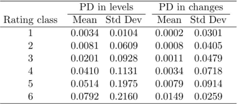
Our study on default risk is in hundreds active corporations in Tehran Stock Exchange. The Tehran Stock Exchange database was used to develop a parsimonious numerical method of modeling and simulating correlated default processes for hundreds of issuers. The empirical ex-amination of the joint stochastic process of default risk was carried out during the period of 1999-2011, and for each issuer, we had PDs based on their econometric models for every semester. The algorithm of Har-tigan and Wong [16] was used for partitioning the data into resembling classes to produce an operational assortment. This method was run us-ing R software (k-means function). Firms were clustered by the k-means method, which aims to partition firms into six groups such that the sum of squares from firms to the assigned cluster centers is minimized. Some issuers fall into rating class 7, which comprises unrated issuers, and the PDs within this class range from high to low. PDs from rating class 7 were not considered. Table 1 reports empirical averages and standard deviations of our data from the first rating class to the sixth rating class. It is obvious from Table 1 that the mean increases from the first rating class to the sixth rating class, as the standard deviation. According to Table 2, Kendall’sτ of default probability of each rating class shows the dependence between rating classes, therefore it needs to joint distribu-tion funcdistribu-tion of rating classes.
Table 1: The results of the time series of average PDs for each rating class. Mean and standard deviation (StdDev) of default probability explained by the common component of default probability are reported both for default probability levels and changes ( PD in changes(t)=PD in levels(t+ 1)-PD in levels(t)=PD in levels(t) ).
PD in levels PD in changes Rating class Mean Std Dev Mean Std Dev
1 0.0034 0.0104 0.0002 0.0301 2 0.0081 0.0609 0.0008 0.0405 3 0.0201 0.0928 0.0011 0.0479 4 0.0410 0.1131 0.0034 0.0718 5 0.0514 0.1975 0.0079 0.0914 6 0.0792 0.2160 0.0149 0.0259
Table 2: Computed Kendall’s τ for default probability of each rating class. Note that the upper right triangle shows the dependence for PD levels. Moreover, the lower left triangle expresses the dependence for PD changes.
Rating class 1 2 3 4 5 6 1 1.0000 0.3125 0.4532 0.2133 0.1963 0.3210 2 -0.2097 1.0000 0.3209 0.1960 0.3317 0.2809 3 -0.1232 -0.2019 1.0000 0.3294 0.1006 0.5919 4 -0.0194 0.0109 -0.3648 1.0000 0.4510 0.3918 5 -0.0930 0.3385 0.4534 0.3289 1.0000 0.3973 6 -0.0978 0.1094 0.1931 0.3893 0.4103 1.0000
3
Copula Functions
Now we define a statistical tool widely and especially used in the finan-cial field, that allows us to express the dependence structure of a vector of variables: the copula. A copula is a statistical tool which has been recently used in finance and engineering to build flexible joint distribu-tions in order to model a high number of variables. ConsiderX1, . . . , Xr
to be random variables andH as their joint distribution function. Then we have the following definition.
Definition 3.1. A r-dimensional copula is a function C : [0,1]r → [0,1] with the following properties:
1. For all (u1, . . . , ur)∈[0,1]r, thenC(u1, . . . , ur) = 0 if at least one coordinate of (u1, . . . , ur) is 0;
2. C(1, . . . ,1, ui,1, . . . ,1) =ui, for all ui ∈[0,1],(i= 1, . . . , r); 3. C is r-increasing, (see Nelsen [22], Definition 2.10.2).
Sklar’s theorem clarifies the role that copulae play in the relation-ship between multivariate distribution functions and their univariate margins.
Theorem 3.1 (Sklar’s theorem). Let H be a joint distribution function with margins F and G. Then there exists a copulaC such that for all x, y in R¯,
H(x, y) =C(F(x), G(y)). (1)
If F and G are continuous, then C is unique; otherwise, C is uniquely determined on RanF×RanG. Conversely, if C is a copula and F and G are distribution functions, then the function H defined by (1) is a joint distribution function with margins F and G (Nelsen [22]).
Hence, if C is a copula, then it is the distribution of a multivariate uniform random vector, as it was stated in Sklar’s theorem and in the corollary derived by Nelsen in 1999, see Nelsen [22]. A copula is thus a function that, when applied to marginal distributions, results in a proper multivariate probability distribution function. Since this pdf embodies all the information about the random vector, it contains all the infor-mation about the dependence structure of its components. Hence by implementing this technique, we split the distribution of a random vec-tor into individual components (marginal) with a dependence structure (the copula) without losing any information. In this paper, the nor-mal and the Student’stcopula are applied. These two types of copulas belong to the class of elliptical copulas. Elliptical copulas are the cop-ulas of elliptical distributions. Archimedean copulae are an alternative to Elliptical copulae . However, to model only positive dependence (or only partial negative dependence), they present the serious limitations while their multivariate extension involve strict restrictions on bivariate dependence parameters. This is why we do not focus on them here.
4
Model Description
Our data were comprised of firms that were categorized into six classes. After using the clustering method for categorizing the data in six rat-ing classes, an attempt was made to study the dependency structure of default for these classes. We averaged across firms within a rating class to obtain a time series of the average intensityλk for eachkrating class. We assumed that the stochastic processes for the six averages λks are drawn from a joint distribution characterized by a copula, which establishes the joint dependence between rating classes. For the inter-pretation of the model and simulation of the joint default process, we also needed the following structure. The rest of the section was orga-nized as follows: Subsection 4.1 introduces a jump diffusion process and Subsection 4.2 explains parameter estimation of marginal distributions and copulas.
4.1 Estimation of the average of each rating class using a Jump Diffusion process
We computed the individual intensity as:
λkj(t) =−log(1−P Dkj(t)), j= 1, . . . , Mk, k= 1, . . . , N, t= 1, . . . , T.
The componentMkdescribes the total number of issuers within the rat-ing class for which data are available in thekth rating class. Moreover, we assume that N = 6 and data size of sample is T (41 sample). Let
λk(t) be the average intensity across rating class kat timet. Therefore,
λk(t) = 1
Mk
Mk j=1
λkj(t), t= 1, . . . , T.
We are now prepared to compute theλk. Letλk(t) follows the stochastic process below:
Δλk(t) =κk(θk−λk(t))Δt+Xk(t), (2) where
Xk(t) =k(t) +Jk(t)Lk(qk, t), k ∼N(0, σ2k), Jk∼N(μk, δ2k),
and
Lk(qk(t), t) =
1 with probability qk
0 with probability 1−qk
Parameters of the jump diffusion process were estimated via Maximum Likelihood Estimation. The jump-sizes were considered to be normal distributed (mean μk and variance δ2k). Here, κk is a parameter con-trolling the speed of mean- reversion of λk. Moreover θk is the level of mean reversion. It was also assumed thatJk,Lkandkare independent. Then residualsXk(t) had a mixture of two normal components. We can depict density function for the residual termXk(t) into the following:
f[xk(t)] =qkf[xk(t)|Lk = 1] + (1−qk)f[xk(t)|Lk= 0], f[xk(t)] =qkfN(μk,σ2
k+δk2)+ (1−qk)fN(0,σ2k).
As we mentioned to simulate (λ1, . . . , λ6) in the first step, we simulated (x1, . . . , x6), and then according to (2) the average of the intensities of each rating class, it can be obtained. When all parameters were estimated, the residuals can be simulated using the copula and marginal distributions of (X1, . . . , X6). For more details about the simulation of intensities see the Appendix.
4.2 Parameter estimation of marginal distributions and
copulas
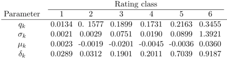
In this step, parameters of the marginal distributions of Xk (residuals) were estimated by the maximum-likelihood method for each rating class. The results of parameter estimation were shown in Table 3. Note that the standard deviation (i.e. δk) increases with declining credit quality. θk
and κk were estimated using data (Das and Geng [6]). After estimating the parameters, residuals for each rating class were computed.
Table 3: Estimated parameters by the maximum likelihood method for the average of the intensities of each rating class.
Rating class
Parameter 1 2 3 4 5 6
qk 0.0134 0. 1577 0.1899 0.1731 0.2163 0.3455
σk 0.0021 0.0029 0.0751 0.0190 0.0899 1.3921
μk 0.0023 -0.0019 -0.0201 -0.0045 -0.0036 0.0360
δk 0.0289 0.0312 0.1901 0.2011 0.7039 0.9187
This approach has been suggested by Das and Geng [6] that their focus is on the classical method, but in this paper two methods were used
to estimate parameters of copulas: the classical and Bayesian method, in addition we have extended it to a mixture of Gaussian distributions for marginal distributions of the residuals of default processes in the classical and Bayesian methods. In order to apply the Bayesian methods for estimation of parameters of copula, we need the posterior distribution, calculated by multiplying the likelihood function to the prior distribution (see the B).
In order to generate a random vector from the copula, first, the dis-tributions of marginal are used, deriving from the residual disdis-tributions (a mixture of Gaussian). Second, a lot of correlation matrices of copu-las were used (i.e. 100000), simulated from the posterior distribution. These matrices were obtained from the MCMC (Markov chain Monte Carlo) method instead of using a fixed parameter estimate of correlation matrices of copulas (see Dalla Valle [4]).
5
Simulating Correlated Defaults
In this section the results of the measure calculated with the classical and Bayesian methods would be shown. Parameters of Student’st and normal copula according to both the classical and the Bayesian methods are estimated then Student’stand normal copula are simulated (see the A) for comparing them with measures in Table 4 in whichdk,t is defined as an element of matrixdas follows:
dk,t=|Rk,t+1−Sk,t+1|, k= 1, . . . ,6, t= 1, . . . ,40,
and measure ¯d
¯
d=
6 k=1
40 t=1dk,t
240 ,
whereRk,t+1 is denoted as the element in the kth rating class and time
t+ 1 of our real data and Sk,t+1 is the element in the kth rating class and the time t+ 1 of matrix S that is obtained from simulated data. Since four methods were applied for these simulations, there are four matrixS. It is obvious that if the measure ¯dis small and it tend to zero, the related simulation of the copula is effective because of two reasons: first, parameter estimation is efficient. Second, in comparison with other copulas, the related copula fits well.
6
Conclusions
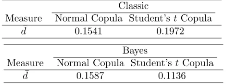
As it is shown in Table 4, Bayesian method in Student’s t copula leads to an improvement of simulation, but it does not in normal copula. This verifies the fact that Bayesian method is not always more efficient than classic one. In this case it is efficient enough for heavy tail distribution. Moreover, our main outcome is that the application of Bayesian method-ology causes a great reduction of measure when copula is Student’s t, but the drawback of the Bayesian method in normal copula compared to the obvious advantage in Student’stis that the reduction is negligible.
Table 4: Results of calculating measures with the classical and Bayesian copulas.
Classic
Measure Normal Copula Student’s tCopula ¯
d 0.1541 0.1972 Bayes
Measure Normal Copula Student’st Copula ¯
d 0.1587 0.1136
As in Table 5 is illustrated, the Student’stcopula is applied with the same correlation matrix and two different degrees of freedom in order to calculate measures. Although calculating measures show that the small degree of freedom improves the simulation, it’s not tangible. The Student’s t copula with high degrees of freedom approximates to the normal copula, therefore according to Table 5, heavy tail distribution fits well on our data.
Table 5: Results of calculating measures using Student’s t copula with the same correlation matrix and two differences degrees of freedom.
Measure Student’stCopula(ν= 13, Σ0) Student’stCopula(ν= 43, Σ0)
¯
d 0.1934 0.1972
Acknowledgements
The authors would like to thank the anonymous reviewers for their valu-able comments and suggestions to improve the manuscript.
References
[1] Cherubini, U., Luciano, E., and Vecchiato, W. (2004), Copula Meth-ods in Finance. New York: Wiley.
[2] Cox, J. C., Ingersoll, J., and Ross, S. (1985), A theory of the term structure of interest rates. Journal of Econometrica, 53, 385-408. [3] Dalla Valle, L. (2012), Erratum to: Bayesian copulae distributions,
with application to operational risk management. Meth. and Comp. in App. Prob.,14, 1121.
[4] Dalla Valle, L. (2009), Bayesian copulae distributions, with applica-tion to operaapplica-tional risk management. Meth. and Comp. in App. Prob.,
11, 95-115.
[5] Dalla Valle, L., Fantazzini, D., and Giudici, P. (2008), Copulae and operational risks. International J. of Risk Assess. and Manag.,9, 238-257.
[6] Das, S. and Geng, G. (2004), Correlated default processes: A criterion-based copula. J. of Invest. Manag., 2, 44-70.
[7] Das, S. and Sundaram, P. (2000), A discrete-time approach to arbitrage-free Pricing of credit derivatives. J. of Manag. Science, 46, 46-62.
[8] Das, S. and Tufano, P. (1996), Pricing credit sensitive debt when interest rates, credit ratings and credit spreads are stochastic. J. of Financial Engineering, 5, 161-198.
[9] Denuit, M., Dhaene, J., Goovaerts, M., and Kass, R. (2005), Actu-arial Theory for Dependent Risk: Measures, Orders and Models. New York: Wiley.
[10] Duffie, D. J. and Singleton, K. J. (1999), Simulating correlated defaults. working paper.
[11] Duffie, D. J. and Singleton, K. J. (2003), Credit Risk: Pricing, Mea-surement, and Management. Princeton: Princeton University Press.
[12] Durante, F. and Sempi, C. (2010), Copula Theory: An Introduc-tion. Bickel, P.(Ed.), Copula Theory and Its Applications, Heidelberg: Springer.
[13] Frey R., McNeil, A., and Nyfeler, M. (2001), Copulas and credit models. International J. of Risk, 4, 111-114.
[14] Genest, C. and Favre, A. C. (2007), Everything you always wanted to know about copula modeling but were afraid to ask. J. of Hydrologic Engineering, 12, 347-368.
[15] Giesecke, K. (2004), Correlated defaults with incomplete informa-tion. J. of Banking and Finance, 4, 1521-1545.
[16] Hartigan, J. and Wong, M. (1979), Algorithm AS136: A k-means clustering algorithm. J. of Applied Statistics, 28, 100-108.
[17] Jarrow, R. A. and Turnbull, S. M. (1995), Pricing derivatives on financial securities subject to credit risk. J. of Finance,50, 53-85. [18] Joe, H. (1997), Multivariate Models and Dependence Concepts.
London: Chapman & Hall.
[19] Lucas, D. J. (1995), Default correlation and credit analysis. J. of Fixed Income,4, 76-87.
[20] Madan, D. and Unal, H. (1999), Pricing the risks of default. Review of Derivatives Research,4, 121-160.
[21] Mari, D. and Kotz, S. (2001), Correlation and Dependence. New York: Imperial College Press.
[22] Nelsen, R. B. (2006), An Introduction to Copulas. New York: Springer.
[23] Robert, C. P. and Casella, G. (2010), Introducing Monte Carlo Methods with R. New York: Springer.
[24] Schonbucher, P. and Schubert, D. (2001), Copula-dependent default risk in intensity models. Working paper, Department of Statistics, Bonn University.
[25] Yu, F. (2004), Correlated defaults and the valuation of default able securities. J. of Finance, 56, 1765-1799.
A
We report below the main steps in order to simulate from a multivariate default process with a given copula. For a detailed review of copula simulation see Dalla Valle et al. [5]. To generate random variables from multivariate default processes, the following algorithm is suggested.
1. Estimate parameters (κkandθk) using real intensities;
2. Determine residuals using equation (2) and step 1;
3. Estimate parameters of the marginal distributions of residuals with numerical method (maximum likelihood method for a mixture of Gaussian);
4. Estimate the parameters of copulas by calculating residuals from step 2;
5. Simulate (x1, . . . , x6) using copula and marginal distributions resid-uals (for more details see Dalla Valle et al. [5]);
6. Finally determine (λ1, . . . , λ6) using simulated (x1, . . . , x6) and equation (2).
B
The copula of the multivariate normal distribution is the normal copula:
C(u1, . . . , ur) = ΦrΦ−1(u1), . . . ,Φ−1(ur)
where C shows the normal copula, Φr implies the joint distribution function of the r-variate standard normal distribution and Φ−1 shows the inverse of the distribution function of the univariate standard normal distribution.
Letx= (Φ−1(u1), . . . ,Φ−1(ur)) named the vector of univariate nor-mal inverse distribution functions, whereui = Φ(xi) fori= 1, . . . , r, and
let Σ named the correlation matrix, then the normal copula probability density function is presented in the following form
c(Φ (x1), . . . ,Φ (xr)) = 1
|Σ|1/2 exp
− 1
2x
Σ−1− I rx
(3)
using equation (3), the normal copula probability density, we calculate the product over t to get the likelihood function using residuals of in-tensity processes, which has the following form:
f(x|Σ) = 1
|Σ|T/2 exp
− T
t=1
1 2x
tΣ−1− Irxt
.
The parameter to be estimated is Σ and we selected the Inverse Wishart distribution as a conjugate prior:
Σ∼InverseWishart (α, B).
Then the posterior distribution is computed using Bayes’ theorem:
π(Σ|x)∼InverseW ishart
T
2 +α;B+ 1 2
T t=1
xtxt
.
We applied the Gibbs sampler algorithm to simulate the correlation matrix’s estimate. We used the 100,000 matrices simulated by the pos-terior distribution obtained with the MCMC method. For more details about parameter estimation of copulas see Dalla Valle [4], Dalla Valle [3], Dalla Valle et al. [5], Genest and Favre [14], Bayesian method see Robert and Casella [23].