TABLE OF CONTENTS
ACKNOWLEDGEMENTS ii LIST OF FIGURES iii LIST OF TABLES iv
ABSTRACT
BRUCE A. PATE. The Monitoring of Underground
Storage Tanks with Passive Dosimetry. (Under the
direction of DR. DAVID LEITH and DR. FRANCIS A.
DIGIANO)
Laboratory tests were conducted to determine the capability
of a dosimeter to measure vapor-phase and aqueous-phase organics.
Satisfactory results led to field testing at the fire training
site at Pope Air Force Base outside of Fayetteville, North Carolina. The dosimeters showed good sensitivity as the vapor-phase dosimeters could measure Ippm after 90 minutes and the aqueous-phase dosimeters could measure 0.2ppm after 5 hours. On
the other hand, the results were not consistent enough to
recommend quantitative monitoring. However, this is believed to
be due more to the sampling methodology employed rather than to
11
ACKNOWLEDGEMENTS
This investigation was conducted as part of a research
program supported by the Water Resources Research Institute of
the University of North Carolina, Grant No. 88-10-70085.
I would like to thank Dr. David Leith and Dr. Francis A.
DiGiano for their guidance during my study in the Department
of Environmental Sciences and Engineering.
I am also grateful to those at Pope Air Force Base who
permitted the use of the fire training site in support of this
LIST OF FIGURES
.Ll
1. Vapor-phase laboratory test of dosimeter 6 2. Design of vapor-phase dosimeter 7
3. Laboratory results of vapor-phase tests 9
4. Field site 11
5. Structure of a permanent vapor well 13
6. Design of an aqueous-phase dosimeter 16 7. Charcoal tube sampling method 20
8. Octane in well VI 26
9. M-xylene in well VI 27 10. 0-xylene in well VI 28
11. Octane in well V2 29
IV
LIST OF TABLES
1. A comparison of JP-4 and gasoline 12 2. Physical properties of the target compounds 17
3. A summary of the methods used to obtain vapor- and 19
aqueous-phase data
4. Vapor measurements for well VI 2 3 5. Vapor measurements for well V2 24
»*!i5"'->\f
INTRODUCTION
In the United States alone, there are between three and
five million underground storage tanks (USTs) which store regulated substances, the most common of which are petroleum products(1). Many of these tanks were installed with the belief that they would never leak, and thus, the possible
deleterious effects of a leak were overlooked. As a result,
there were over 100,000 leaking underground storage tanks
(LUSTs) in 1985 and more than 300,000 were expected to be
leaking by 1990(2).
To deal with this problem, the EPA was required to
promulgate UST standards in accordance with the 1984 Hazardous and Solid Waste Amendments to the Resource Conservation and
Recovery Act. A tank must have at least ten percent of its
volume (including piping) underground and contain a regulated
substance to be considered an UST by the EPA(3). Exemptions
include residential fuel tanks less than 1100 gallons, septic tanks and heating oil tanks. The Office of Underground Storage
Tanks (OUST) was established by the EPA to administer and create the necessary regulations. At present, all piping is
required to be monitored for leaks by December 1990, and all
tanks by 1993(4).
The financial and environmental consequences of a leaking
tank can be enormous. The average cleanup cost is $70,000
surface water becomes contaminated, then the costs become
exorbitant. In fact, each tank today is required to carry one million dollars of insurance per possible occurrence(6). Thus, to minimize possible environmental and financial costs, an effective leak detection progam is of vital importance.
Many leak detection methods are available. These
procedures range from simple inventory control or volumetric testing to the employment of sophisticated equipment using
lasers or x-ray fluorescence. Regardless of the method used,
the processes of determining the existence of a leak, the leak rate and its pathway, are complicated. As a result, there is no single preferred procedure as each has good and bad
features(7).
Passive dosimeters have long been used in the nuclear industry and have also become an important industrial hygiene tool for monitoring noxious inorganic gases and volatile
organic compounds. However, only recently have passive
samplers been used outside of the industrial environment. In 1986 Kerfoot and Mayer used passive samplers in their soil-gas survey of a site in Nevada contaminated with chloroform(8). Their samplers showed a correlation of greater than 99% significance with grab-sampling measurements and gave an
"accurate picture of the ground water contamination at the
OBJECTIVES
1. To execute vapor-phase laboratory tests of passive
dosimetry.
2. To develop vapor-phase and aqueous-phase dosimeters
suitable for field testing.
3. To conduct field testing of the dosimeters. 4. To analyze the field results and recommend applications of passisve dosimetry in the monitoring
of underground storage tanks.
THEORY
Unlike conventional methods of collection, passive dosimetry requires no active parts or energy input since it operates on the principle of molecular diffusion for the transport of contaminant to the collecting surface. Assuming steady-state conditions, where molecular concentrations do not change with time, this process can be described using Pick's
first law of diffusion:
J= -D dc/dx (1)
where: J= contaminant mass flux (ng/cm^s)
0= diffusion coefficient of contaminant (cmVs)
dc/dx= concentration gradient (ng/cm') along
diffusion pathlength (cm)
Substituting (C, - Co)= dc, the change in concentration over
the pathlength, and -I> (X, - Xq)= dx, the diffusion
J= (D/L) (C, - C,) (2)
where: L= diffusion pathlength (cm)
C,= ambient concentration of contaminant (ng/cm')
Cj,= contaminant concentration at the
collecting surface
Since the sorbent, granular activated carbon(GAC), tightly
binds most organic constituents, C^ can be assumed to be zero,
i.e., the dosimeter has a 100% collection efficiency.
Multiplying both sides of equation (2) by time and area gives: M= (D/L) AC.t (3)
where: M= contaminant mass collected (ng)
A= cumulative cross-sectional area of the diffusion channels (cm^)
t= time of exposure (s) The mass collected (M) is given by:
M= m/EF (4)
where: m= contaminant mass detected from GC analysis E= extraction efficiency of solvent
F= instrument response factor
The average ambient concentration can be calculated by rearranging equation (3) to give:
C,= (ML)/(DAt) (5)
Two of the parameters, length and area, are physical
dimensions of the dosimeter and are accurately known, as is
the time of exposure. The diffusion coefficient, which is
pressure, remains relatively constant during field tests. Thus, the only significant uncertainty associated with
equation (5) is the calculation of M, which is determined experimentally in the laboratory.
If the ambient concentration varies rapidly, then the dosimeter may not be able to respond quickly enough to give accurate results. Hearl and Manning showed that the dosimeter
will be accurate if t<<LVD, where t is the time between
significant changes in concentration(9). In this study, lVd
varied from .15 seconds for the aqueous phase to 16 seconds for the vapor phase. Thus, unless the ambient concentration changes every few seconds, the dosimeter will give
representative results. Since ground water and soil vapor
concentrations change slowly, this concern did not affect this
study.
LABORATORY TESTING OF THE DOSIMETER
A laboratory experiment, seen in Figure 1, was conducted to determine what concentration a dosimeter would predict in a relatively stagnant situation, which would be analogous to the planned vapor-phase field tests. A prototype dosimeter 7.5 cm across, made of an acrylic polymer, with 1.0 cm length
channels and a diffusion area of 3.75 cm^, was placed on a
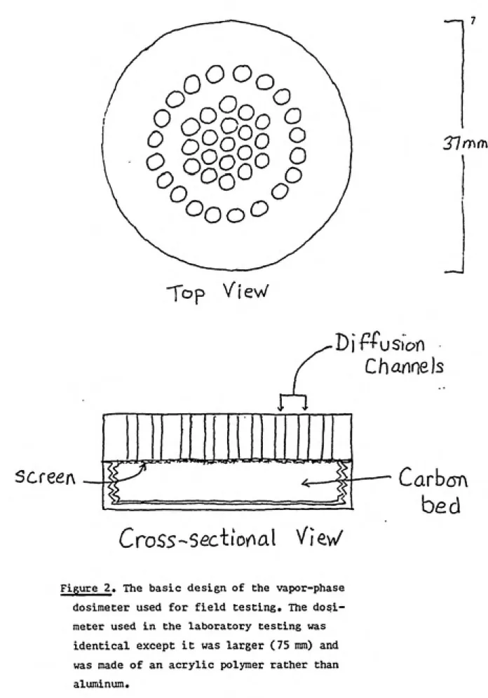
simple cardboard stand in an 8 liter dessicator. The basic design of the prototype dosimeter can be seen in Figure 2, which gives the design of the dosimeter used in the field
1 ppm
Octane -^
^
Do5i'meter
Figure l«The laboratory testing of the vapor-phase
dosimeter was conducted in a dessicator. Octane at
a concentration of 1 ppn was added at a rate of 50 scfh for two minutes, at which time a 1 ppm
concentration was established in the dessicator.
The system was then sealed and the dosimeter was
exposed for varying lengths of time. The purpose of this test was to determine how the dessicator
0 gSgog O
screen
OqoO
"fop VieW
31n\(T\
_J
Channels
Carh(m
bed
Cross-Seciiof^al Viev/
Figure 2. The basic design of the vapor-phase
dosimeter used for field testing. The dosi¬ meter used in the laboratory testing was
identical except it was larger (75 mm) and
grease was used to form a seal between the lid and the
dessicator.
The system was flooded with 1 ppm octane from a
compressed gas cylinder at a 50 scfh flow for two minutes to
establish a 1 ppm concentration. At this time the dessicator
was closed off and allowed to sit for 50 to 12 0 minutes. The
carbon (Ig) was desorbed with 10 ml CSg and spiked with
m-xylene, which served as the internal standard for the gas
chromatographic analysis. Appendices A and B outline the
procedures for recovery of the contaminant and the
standardization of the gas chromatograph.
The results were fairly consistent, with decreasing
average concentration with increasing time(Figure 3). This was
due to the concentration inside the dessicator decreasing
significantly as the dosimeter removed more and more octane.
The dosimeter removed less than 8% of available octane after
60 min and less than 9% after 80 min. While this procedure was
not a perfect test, the results were believed to be a
reasonable indicator of how the dosimeter performed in a
quiescent atmosphere.
The feasibility of using passive dosimetry for
aqueous-phase monitoring was determined with a series of laboratory
experiments in an adjunct research project(lO). Toluene,
ethylbenzene and m-xylene were added to a 53.5 liter Nalgene
polyethylene tank filled with tap water. Three dosimeters were
placed in the tank and the results obtained were consistently
Vapor-Phase Test of Dosimeter
g.
a
c
o U (4 U d 0) u
c
o
0.9-Time (minutes)
Figure 3. Laboratory results of dosimeter vapor-phase
sampling of octane in a quiescent atmosphere. (The vertical bars represent the data range at:a
10
FIELD SITE
Field work was conducted at the fire training site at Pope Air Force Base outside of Fayetteville, North
Carolina(Figure 4). The central part of the training site
consisted of a circular, 3 foot sand barrier approximately 135 feet across. The pit contained no liner and had a pool of
water with a layer of JP-4 jet fuel floating on top. There was also a thick non-aqueous-phase hydrocarbon layer just above the water table. Table 1 compares the distribution of
components of JP-4 with gasoline as measured by gas
chromatography(12). Prior to a burn, JP-4 would be pumped into the pool of water. Since the site has been in use for many decades, and the water table was only 4-6 feet below the pit, there was a significant contamination of the surrounding area.
The site was surrounded by permanent wells established by University of North Carolina study teams which were used to take groundwater and vapor measurements(Figure 5). The vapor wells, labeled "V, had a three inch metal casing which
extended into the groundwater. The casing had a hole drilled 20 inches below the top end and at 12 inch increments
thereafter. Metal tvibing(l/8 inch diameter) was attached to each hole and stretched to the surface to take vapor
ALDISH RD.
POPE AIR FORCE BASE
NORTH CAROLINA
FIRE TRAINING AREA mFT5 O
O V3
O O FT1
0 permanent sampling wells
ͫ
temporary sampling well VI
/^ temporary saunpling well V2 Test Days 3-5
4 temporary sampling well V2 Test Days 6-11
"TI non-aqueous-phase
/} hydrocarbon layer
NORTH
Scalsi laa*
Figure ^. Field testing site. Pope Air Force Base, Fayetteville, North Carolinadl)
12
compound mol. wt. fa/mol) a3re?i% JP-^ area% aas.
propane 44.04 1.00 2.10
isobutane 52.18 2.65 6.00
n-butane 52.18 5.60 32.50
methyl butane 72.15 12.25 21.80
n-pentane 72.15 13.05 10.90
dimethyl butane 86.18 2.45 1.90
methyl pentane 86.18 11.30 5.50
n-hexane 86.18 8.15 2.30
methyl cyclopentane 84.16 3.45 1.00
benzene 78.12 1.25 .50
cyclohexane 84.16 3.10 .30
methyl hexane 100.21 2.70 .50
dimethyl pentane 100.21 2.70 .00
n-heptane 100.21 4.30 .40
methyl cyclohexane 98.19 2.75 .00
toluene 92.15 1.15 .90
methyl heptane 114.23 1.50 .00
dimethyl cyclohexane 112.22 1.50 .00
n-octane 114.23 2.00 ,10
ethyl benzene 106.17 .18 .20
xylenes 106.17 .68 .55
<fOOrtd Sor'ffluie
Frcrfecfi ^^e Co\/cr
7,0 inches
\A
CO£>it\
IS In^-hfi
12 /nclie5
^ Tc«i
13
5 inches
Figure 5« Basic design of permanent vapor-phase sampling
wells VI and V2, The aqueous-phase sampling well, FT6,
14
The soil was composed of medium sand particles to a depth of 8-10 inches, before becoming mixed with a small amount of clay. The soil in the woods nearby had a much higher organic
content in the top layer and hard clay at a depth of about 12
inches. During the testing period from March 15, 1989 to June
9, 1989, there was a large amount of rain which raised the
water table 24-26 inches.
MATERIALS
New dosimeters were made from aluminum since the original
design used an acrylic polymer that was capable of absorbing hydrocarbons. While this would not be a problem for the vapor
measurements, there was a thick hydrocarbon layer floating on
the aquifer which could irreversibly damage the dosimeters used for aqueous-phase sampling. Both the vapor-phase and aqueous-phase dosimeters had a diameter of 37 mm and were composed of two pieces that screwed together.
The top-half of the vapor-phase dosimeters contained 39
diffusion channels, each 1 cm in length and 0.05 cm^ in
cross-sectional area, giving a total area of 1.95 cm^(Figure 2).
This section was backed by a 30 mesh screen to prevent loss of
carbon. The top-half also contained a hollowed space which
held 0.8 g of carbon and an o-ring around its edge to
establish an effective seal. The bottom served as a screw-on
cap which held the carbon in place.
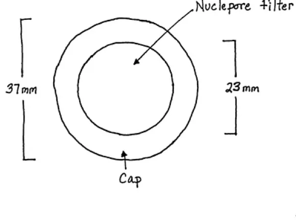
The bottom-half of the aqueous-phase dosimeter had a
15
carbon(Figure 6). A polycarbonate Nuclepore filter was placed over the carbon and served as the diffusion barrier. The
filter was 10 um thick with 7.9% open surface area, which was
determined using a scanning electron microscope(Appendix C).
Since the filters were too wide, they were cut from 37 mm to 32 mm. A small hole was drilled through the center of the dosimeter and a 10 mm Supelco microsep septum was placed on
the backside. This design allowed the needle of a syringe to
pass into the carbon bed to draw water through the filter and
eliminate any air pockets beneath it. A screw-on cap, with an
open center which matched the hollowed space of the bottom half, held the filter in place.
The GAC used was Calgon Filtrasorb 400. It was ground to 20-30 mesh and washed with distilled water to remove all fine particles. The carbon used in the water analysis was boiled
for 30 minutes and stored in water. This was done to remove air from the carbon pores which could reduce the carbon's adsorptive efficiency.
SELECTION OF TARGET COMPOUNDS
Three constituents of JP-4; n-octane, m-xylene and o-xylene,
were targeted since they gave clean peaks on the chromatogram and they represented alkane and aromatic compounds. The
physical characteristics of the target compounds are listed in Table 2. Thus, these chemicals were used in the laboratory to establish carbon desorption efficiencies and instrument
16
r
31m(r\
\
f\oc\tf(rrt filier
23 mm
-fiWev
S
Carbcm hed
(drills h<?l<
17 were of reagent grade. Carbon disulfide was used to desorb
organic constituents from the GAC and 1-chloroheptane was
employed as the internal standard. Sodium sulphate was used as
a drying agent.
Table 2. Physical properties of the target compounds
compound
mol. wt. fa/mol)
114
density
0.703
boil, pt. dif. CO aii:^'
0.062
ef. (cmVs) sol. water^* fma/1)
octane 126 5.63E-6 0.66
m-xylene 106 0.868 138 0.069 6.71E-6 175 o-xylene 106 0.870 142 0.073 6.71E-6 175
METHODS OF SAMPLING
Two temporary wells were dug near permanent wells VI and
V2 for the obtaining of vapor measurements(Figure 4). Wells VI
and V2 were chosen because they were in the region of highest
concentration which permitted the largest number of samples to
be taken during a Test Day. The temporary wells were dug with
a post hole digger and were six inches in diameter. At the end
of each Test Day, the wells were refilled. The temporary well
located near (40 inches) well VI was dug to a depth of 17.5
inches for all Test Days to correspond to the highest drilled
hole of well VI. The temporary well located near (69 inches) well V2 was dug to a depth of 27 inches to correspond to the
second highest drilled hole of V2. However, because of rising
ground water levels, a new hole, 38 inches from V2, was dug to
18
6-11. Table 3 summarizes and labels the various methods used
to measure field concentrations.
The GAC for each dosimeter sample(VP/D) was placed in
separate vials in preparation for each trip (except for Test
Days 3 and 4 in which the carbon was dispensed from a single
vial). At the test site, the contents of a vial were poured
into a dosimeter, the two halves were screwed together, then
the dosimeter was pressed against the side of the well. Care
was taken to ensure no gap was present between the dosimeter
face and the soil. After 90 minutes (well VI) or 75 minutes
(well V2), the dosimeter was removed and the carbon was placed
into its vial.
At some point during the day, measurements(VP/CT/PW) were
taken from the permanent vapor wells to serve as a "standard"
to which the dosimeter results could be compared. This was
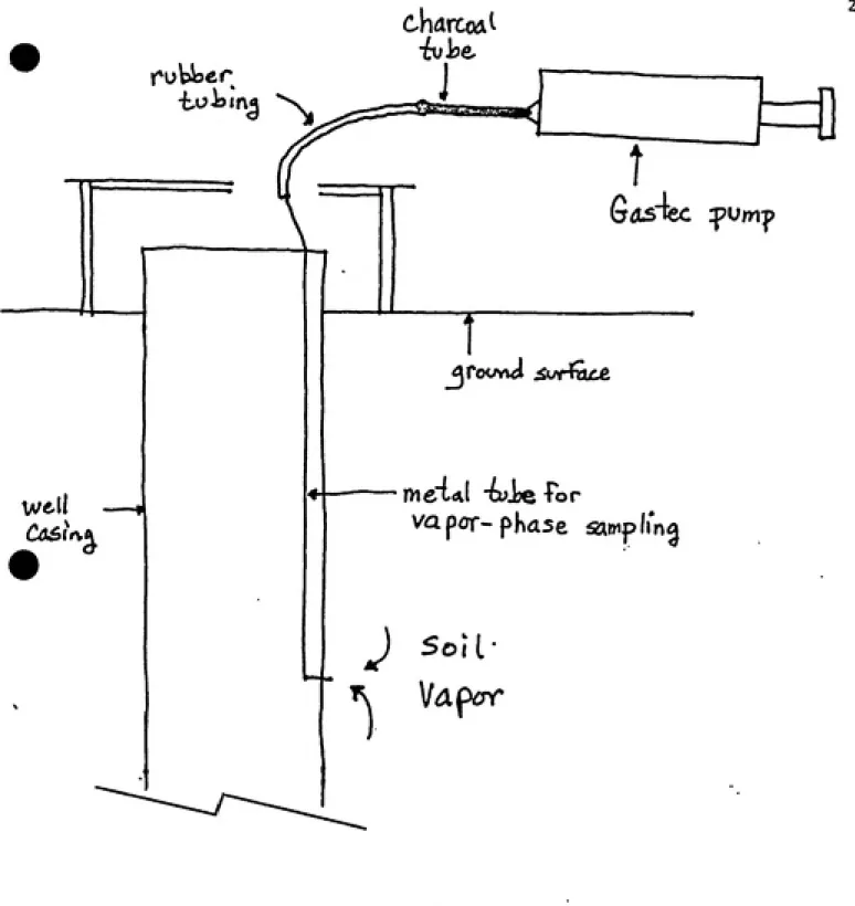
done by using 400 mg/200 mg SKC charcoal tubes and a 100 cc
Gastec precision gas detector system(Figure 7). First, 200 cc
of air was pumped from the metal tube, then the charcoal tube
was attached and 200 cc were drawn slowly through. After the
tube was removed and capped, the procedure was repeated with a
second tube. Used charcoal tubes were placed in a small
cooler, and upon returning, they were frozen until analysis,
usually 3-4 days later.
For Test Days 8-11, "standard" measurements(VP/CT/TW)
were taken from the temporary well where the dosimeter was
located. A thin piece of cardboard was placed along the side
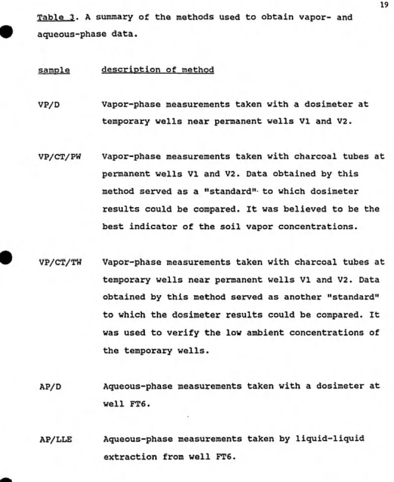
Table 3. A summary of the methods used to obtain vapor- and
aqueous-phase data.
19
sample description of method
VP/D Vapor-phase measurements taken with a dosimeter at
temporary wells near permanent wells VI and V2.
VP/CT/PW Vapor-phase measurements taken with charcoal tubes at
permanent wells VI and V2. Data obtained by this
method served as a "standard" to which dosimeter
results could be compared. It was believed to be the best indicator of the soil vapor concentrations.
VP/CT/TW Vapor-phase measurements taken with charcoal tubes at
temporary wells near permanent wells VI and V2. Data
obtained by this method served as another "standard"
to which the dosimeter results could be compared. It was used to verify the low ambient concentrations of
the temporary wells.
AP/D Aqueous-phase measurements taken with a dosimeter at well FT6.
20
jrowwsl jStY^ftlC^
mex«*( -^jic Tor
vapor-phase sawfli'n^
Figure 7. Method employed for obtaining vapor samples from
permanent wells VI and V2, All VP/CT/PW samples were collected
21
into the soil. A two inch, 19 gauge needle was fastened to a
piece of rubber tubing which was connected to the pump. The
needle was punched through the cardboard at the bottom of the
well. After 200 cc of air was removed the charcoal tube was
attached. No results were obtained during Test Days 8 and 9 because not enough air was pumped. For Test Day 10, 800 cc of air were pumped from the soil and for Test Day 11, 1000 cc of
air was removed.
The dosimeter used for water measurements(AP/D) was
filled with GAC, covered with a nuclepore filter, and capped. The dosimeter was submerged in water and the needle of a
syringe was passed through the septum on the bottom of the dosimeter. Water was drawn through the dosimeter and into the syringe to remove the air pockets that formed between the filter and the carbon bed. The dosimeter was then placed in well FT6 for 4.5-5 hours. After this time, the dosimeter was
removed from the well and the carbon was placed in a vial. To obtain a measurement(AP/LLE) to serve as a standard
concentration, a 40 ml vial was used to draw out water from the well. Enough water was removed to make two 60-70 ml samples which were analyzed after a liquid-liquid
extraction(LLE).
RECOVERY OF CONTAMINANTS
The VP/D samples were analyzed 1-2 days after each field
test. To each vial was added 9 ml CSj which had been spiked
22 the charcoal tubes(VP/CT/PW and VP/CT/TW) were placed in
separate vials with 6 ml and 2 ml CS2 being added
respectively. At least 30 minutes were allowed for desorption.
The AP/D samples had 8 ml spiked CSj and 1 g sodium sulphate added and were allowed to stand (with intermittant shaking) for several hours before analysis. Each AP/LLE
sample(removed from the well with a vial) was placed in a 250
ml separatory funnel with 12-15 ml of unspiked CSj. The
mixture was shaken and allowed to settle before the CSj layer
was drained into a 15 ml Erlenmeyer flask. The extract was spiked with the internal standard and 1 g of sodium sulphate was also added. A liquid-liquid extraction efficiency of 100%
was assumed.
Aliquots of 0.9 ul were injected into a Varian 3700 Aerograph gas chromatograph equipped with an FID and an SP-2100 fused silica capillary column. All samples were run with the same temperature program; five minutes at 60"?, then
ramped at 4°F/min to an end temperature of 78"?. Although
JP-4 is a complex mixture, the vapor-phase chromatograra was made relatively simple by the low vapor pressures of the heavier organics. The aqueous-phase chromatograms were simplified by the low solubilities of the aliphatic constituents.
RESULTS
The results of the vapor-phase measurements for octane, m-xylene and o-xylene are given in Tables 4 and 5, in which
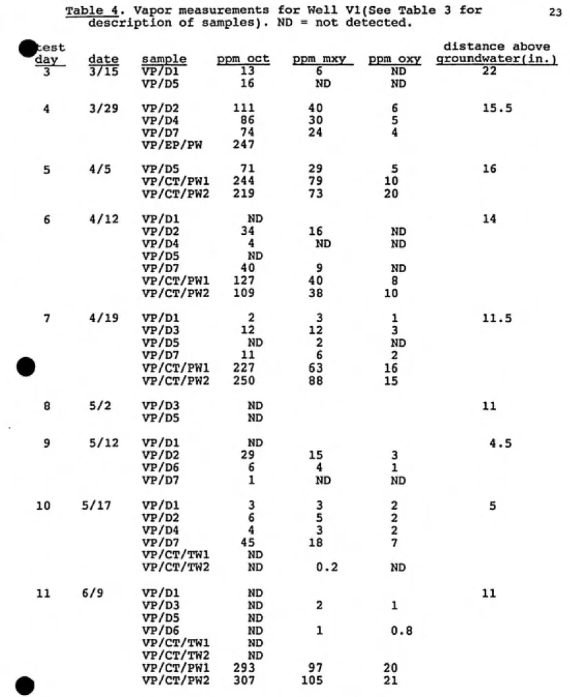
Table 4. Vapor measurements for Well VI(See Table 3 for 23
description of samples). ND = not (detected.
^est distance above
day date sample ppm oct ppm mxy ppm oxy qroundwater(in.)
3 3/15 VP/Dl 13 6 ND 22
VP/D5 16 ND ND
4 3/29 VP/D2 111 40 6 15.5
VP/D4 86 30 5
VP/D7 74 24 4
VP/EP/PW 247
5 4/5 VP/D5 71 29 5 16
VP/CT/PWl 244 79 10
VP/CT/PW2 219 73 20
6 4/12 VP/Dl ND 14
VP/D2 34 16 ND
VP/D4 4 ND ND
VP/D5 ND
VP/D7 40 9 ND
VP/CT/PWl 127 40 8
VP/CT/PW2 109 38 10
7 4/19 VP/Dl 2 3 1 11.5
VP/D3 12 12 3
VP/D5 ND 2 ND
VP/D7 11 6 2
» VP/CT/PWl 227 63 16
VP/CT/PW2 250 88 15
8 5/2 VP/D3
VP/D5
ND
ND
11
9 5/12 VP/Dl ND 4.5
VP/D2 29 15 3
VP/D6 6 4 1
-VP/D7
I ND ND
10 5/17 VP/Dl 3 3 2 5
VP/D2 6 5 2
VP/D4 4 3 2
VP/D7 45 18 7
VP/CT/TWl ND
VP/CT/TW2 ND 0.2 ND
11 6/9 VP/Dl ND 11
VP/D3 ND 2 1
VP/D5 ND
VP/D6 ND 1 0.8
VP/CT/TWl ND
VP/CT/TW2 ND
VP/CT/PWl 293 97 20
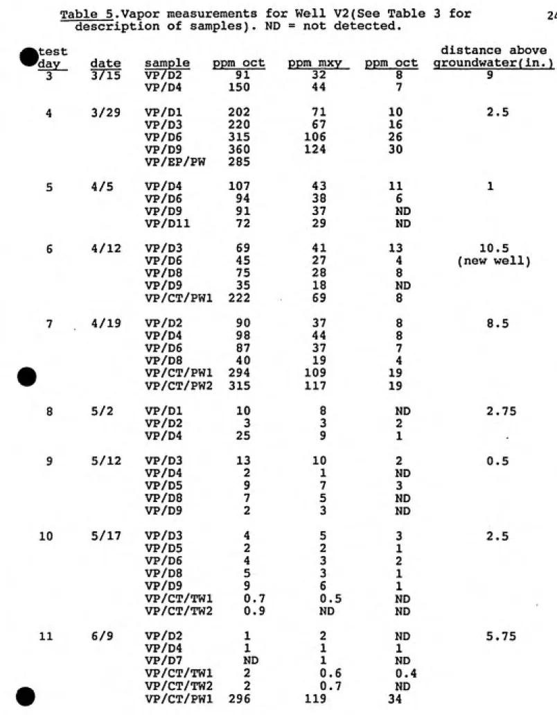
Table 5.Vapor measurements for Well V2(See Table 3 for description of samples). ND = not detected.
24
ktest
^day date
3 1715
3/29 4/5 4/12 4/19 5/2 5/12 10 5/17 11 6/9
sample ppm oct ppm mxy ppm oct
VP/D2 91 32 8
VP/D4 150 44 7
VP/Dl 202 71 10
VP/D3 220 67 16
VP/D6 315 106 26
VP/D9 360 124 30
VP/EP/PW 285
VP/D4 107 43 11
VP/D6 94 38 6
VP/D9 91 37 ND
VP/Dll 72 29 MD
VP/D3 69 41 13
VP/D6 45 27 4
VP/D8 75 28 8
VP/D9 35 18 ND
VP/CT/PWl 222 69 8
VP/D2 90 37 8
VP/D4 98 44 8
VP/D6 87 37 7
VP/D8 40 19 4
VP/CT/PWl 294 109 19
VP/CT/PW2 315 117 19
VP/Dl 10 8 ND
VP/D2 3 3 2
VP/D4 25 9 1
VP/D3 13 10 2
VP/D4 2 1 ND
VP/D5 9 7 3
VP/D8 7 5 ND
VP/D9 2 3 ND
VP/D3 4 5 3
VP/D5 2 2 1
VP/D6 4 3 2
VP/D8 5 3 1
VP/D9 9 6 1
VP/CT/TWl 0.7 0.5 ND
VP/CT/TW2 0.9 ND ND
VP/D2 1 2 ND
VP/D4 1 1 1
VP/D7 ND 1 ND
VP/CT/TWl 2 0.6 0.4
VP/CT/TW2 2 0.7 ND
VP/CT/PWl 296 119 34
25
samples were obtained with the dosimeter, the VP/CT/PW samples
were taken from the permanent wells, and the VP/CT/TW samples were taken from the temporary wells. The VP/EP/PW data for Test Day 4, is an average of the samples taken from the
permanent wells with an electric pump. These measurements were
taken on the same day as part of another research project. The last column refers to how far above the groundwater the
dosimeters were placed and gives some indication of how much the water table rose during the field work.
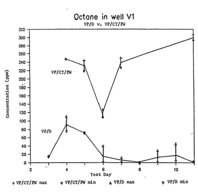
A comparison of the vapor-phase concentrations measured by VP/D and VP/CT/PW at well VI can be seen in Figures 8 to
10. A similar comparison at well V2 can be seen in Figures Il¬ ls. Although the VP/CT/PW concentrations remained relatively constant, there was significant variation of the dosimeter results from Test Day to Test Day as well as during a single day. The dosimeter data collected during Test Day 4 is unusual
in that the concentrations are extremely high. While there is no suitable explanation for the sharp increase, it should be considered that this was the only test during which JP-4 was pumped into the burn pit. The VP/CT/PW data for Test Day four
in Table 4 is also notable. The charcoal tubes had a large amount of contaminant adsorbed in the back-up section which affect the credibility of the results(15).
The results of the aqueous-phase measurements are given in Table 6. The AP/D samples were measured with the dosimeter and the AP/LLE samples were obtained by liquid-liquid
26
I.
a c o
•l-l u
nJ U
XJ
C 0) o c o u
Octane in well V1
VP/D V. VP/CT/PW
VP/CT/PW
Test Day
+ VP/CT/PW max ^ VP/CT/PW rain ^ VP/D max
10
7 VP/D min
Figure 8. A comparison of dosimeter results for octane
with those obtained by the charcoal tube and pump
27
i
c o
U c o fi o o
110
M-xylene in well V1
VP/D V. VP/CT/PW
100 -^
VP/CT/IW
+ VP/CT/PW max
5 6 7 8 Test Day
« VP/CT/PW min ^ VP/D max
r
10 11
7 VP/D min
Figure 9. A comparison of dosimeter results for m-xylene with those obtained by the charcoal tube and pump
28
a,
c o
•H U
nj
c
u c o
0-xylene in well VI
VP/D V. VP/CT/EW
VP/CT/PW
+ VP/CT/PW max
Test Day
« VP/CT/PW min ^ VP/D max 7 VP/D rain
Figure 10. A comparison of dosimeter results for 6-xylene
with those obtained by the charcoal tube and pump
29
o. c o
•H
(4 U
4J
fl
0) o
c
o o
400
350
300
-
250-
200-150-i>
100
-
50-Octane in well V2
VP/D V. VP/CT/PW
VP/CT/PW
+ VP/CT/PW max
Test Day
« VP/CT/PW min a VP/D max 7 VP/D min
Figure 11. A comparison of dosimeter results for octane
with those obtained by the charcoal tube and pump
30
a a
(3
O
u u c o
o
M-xylene in well V2
VP/D V. VP/CT/PW
120 110 00
-VP/CT/PW
50
-+ VP/CT/PW max
Test Day
« VP/CT/PW min & VP/D max ͣ7 VP/D min
Figure 12. A comparison of dosimeter results for m-xylene
with those obtained by the charcoal tube and pump method using permanent well V2. (The vertical bars
31
a
c o
4J
nj !-i
4J
C UJ o c o o
0-xy!ene in well V2
VP/D V. VP/CT/PW
VP/CT/PW
Test Day
+ VP/CT/IVf max o VP/CT/PW rain ^ VP/D max 7 VP/D min
Figure 13., A comparison of dosimeter results for o-xylene
with those obtained by the charcoal tube and pump
method using permanent well V2. (The vertical bars
32
Table 6. Aqueous-phase measurements of target compounds
for well FT6.
test day date 3/29 4/5 4/12 4/19 5/2 5/12
sample ppm mxy ppm oxy
AP/D 0.73 0.48
AP/LLEl 1.24 0.98
AP/T,LE2 0.92 0.78
AVG LLE 1.08 0.88
DF/AVG LLE 0.68 0.55
AP/D 1.80 1.12
AP/LLEl 1.61 1.27
AP/LLE2 2.01 1.69
AVG LLE 1.81 1.48
DF/AVG LLE 0.99 0.76
AP/D 1.20 0.80
AP/LLEl 2.64 2.04
AP/LLE2 3.62 3.09
AVG LLE 3.13 2.56
DF/AVG LLE 0.38 0.31
AP/D 0.39 0.33
AP/LLEl 2.27 1.87
AP/LLE2 1.41 1.18
AVG LLE 1.84 1.52
DF/AVG LLE 0.21 0.22
AP/D 0.22 0.14
AP/LLEl 1.08 1.10
AP/LLE2 1.33 1.29
AVG LLE 1.20 1.20
DF/AVG LLE 0.18 0.12
AP/D 0.24 0.26
AP/LLEl 0.40 0.53
AP/LLE2 0.36 0.51
AVG LLE 0.38 0.52
DF/AVG LLE 0.63 0.50
water level
(inches below ground)
33
samples. The DF/AVG LLE denotes the ratio of the dosimeter to the average of the LLE measurements. This ratio varied but was
always less than one. A comparison of AP/D and LLE
measurements can be seen more clearly in Figures 14 and 15. The last column in Table 6 gives the number of inches below the ground surface that the water table was measured.
DISCUSSION
From Figures 8 to 13 it can be seen that the
concentration of target compounds measured by the dosimeter were far lower than those obtained in the permanent wells using the Gastec system. This comparison is important because the VP/CT/PW data is the best indicator of what the actual soil~vapor concentration might be. There were undoubtedly many factors leading to this difference. Perhaps most important is that the ambient concentration that the dosimeter was exposed to was probably much less than the true vapor-phase
concentration. This could have been due to the mixing of soil vapor with outdoor air that occurred each time the temporary wells were dug. Mixing due to the movement of outside air into
the well during exposure was also considered to be a
contributing factor. However, the data from Test Days 8-10, in which the wells were covered, did not show an increase as
would be expected if dilution with outside air were a problem
during a run.
34
3,5
-a
a
o •rl
U
(6 U U
c u
(3
O o
2.5
1.5
-
0.5-Water measurements of m-xylene
AP/D V. AP/LLE
AP/LLE
+ AP/LLE max
Test Day
^ AP/LLE min AP/D
Figure 14« A comparison of dosimeter results for m-xylene with those obtained by liquid-liquid extraction from
35
a
c o
.1-1
j-> nj U
i->
c <u o c o
Water measurements of o-xylene
AP/D V. AP/LLE
0.6-+ AP/LLE max
Test Day
^ AP/LLE min AP/D
Figure 15. A comparison of dosimeter results for o-xylene
with those obtained by liquid-liquid extraction from
permanent well FT6. (The vertical bars represent the
36
verified when the Gastec system was used for measuring the temporary wells. The data from these measurements(VP/CT/TW) can be seen in Tables 4 and 5. Even though the method for obtaining this data was identical to that used for the VP/CT/PW data, four to five times more air was required to adsorb enough contaminant to even analyze, since the amount adsorbed was far less than that obtained from the permanent wells. While some dilution from outside air probably occurred, there is little doubt that the ambient concentration around
the temporary wells was reduced.
Other possible contributing factors are theoretical. For a dosimeter to give representative results, a minimum face velocity is required (16,17,18). However, in this study the dosimeters were pressed against the side of a well so that there would be minimal movement of air across the face. When the air being measured is relatively stagnant, the diffusion channel length is essentially extended and the ambient
concentration at the dosimeter face is reduced (Figure 16). This lengthening occurs because as the dosimeter removes the
ambient organics, there is insufficient movement of
contaminant to replace what was adsorbed. In other words, the steady-state requirement of Pick's First Law has been
breached.
While stagnant air does present problems for the dosimeter, the laboratory tests indicate that reasonable
37
DlFFU5lOM
PoSlAiBTEl? FACE
SOIU
0EP
I
DlFFUSXOh^
Figure 16. Diagram 16a shows how the dosimeter operates under ideal conditions, DiagraJti 16b shows what can happen when there is insufficient flow across the dosimeter face. Since the adsorbed organics are not being replaced, the
38
the dosimeter can give reasonable results in the field as well. Unfortunately, there are not enough VP/CT/TW
measurements to draw any solid conclusions.
The aqueous-phase dosimeters gave a fairly good
comparison of target compound concentrations to those measured by LLE. As can be seen from Figures 14 and 15, the target
concentrations rose and then decreased. Since there was a
significant increase in the water table, a drop in the ambient concentration might be expected because of dilution. However, this reasoning is not supported by the data. For example, the concentration between Test Days 4 and 6 tripled even though the water level remained relatively constant. Thus, if it is possible for a large increase in concentration to occur
without a change in the water level, then it may also be possible for a large decrease in concentration with a change
in the water level.
A better explanation for the decrease in concentration is that stagnant water was being measured(Figure 17). As water levels rose, the water in the well ascended past the screened portion. This created a volume of immobile water in which the contaminant concentration was significantly less, as seen by the disappearance of the hydrocarbon layer inside the well. Since the water used for liquid-liquid extraction came from the stagnant layer, it provided a good indication of how much the sampling was affected by the rising water table.
39
17a
17b
Coell
I
gspaogssEBsssEE
I
J
Nov-Aqueous
HYT>flOCfiif30NS
LEVEL.
t
ST^e^^ANT
LaysR <Ca
screened
Figure 17. Diagram 17a shows well FT6 under normal
operating conditions. In diagram 17b, the rising water level is above the screened portion and there is no non-aqueous-phase hydrocarbon layer present. Since there is no groundwater flow above the screen, a stagnant layer of water forms in the well in
which the concentration is reduced.
ͣ
* 1 ͣ 9ia A
40
lower in the well than outside, then the dosimeter data for
Test Days 7 and 8 should have been a much higher ratio of AVG LLE. However, the dosimeter was not placed at the same depth for each test. The fact that the dosimeter measurements were
lower than the LLE measurements for Test Days 7 and 8 could
have been due to the dosimeter being in the stagnant layer as well. As the dosimeter removed the available xylenes, there
was no influx of new hydrocarbons to replace what was adsorbed
and the ambient concentration quickly diminished.
It is interesting to compare the data for Test Days 8 and
9. Even though the LLE measurements were reduced by a factor of three, the m-xylene concentration remained constant while
the o-xylene concentration nearly doubled. The decrease in thu
measurements were probably due to the increased stagnation and
dilution as the water level rose five inches in the ten days
between tests. A corresponding decrease in the dosimeter data would be expected but did not occur. This could have been the
result of the dosimeter being placed closer to the screened
portion for Test 9.
CONCLUSIONS
Passive dosimetry can be a useful qualitative tool for the mapping of a contaminated area. If the extent of
contamination at a site was unknown, this method could be ur.c<l
to get a relatively easy and quick determination of the
problem. The dosimeters showed good sensitivity by measuring
41
90 minutes and 0.2 ppm in the aqueous-phase after 5 hours. The sensitivity can be increased easily by allowing longer
exposure times. Another advantage is that there would be no disruption of service while monitoring.
However, the vapor-phase results are not consistent enough for the method to be used quantitatively. This may be due more to the sampling methodology employed rather than to
limitations of passive dosimetry. The vapor-phase measurements could be improved if a vapor manifold assembly, similar to what Kerfoot and Mayer used, was implemented in the field tests(19). Their assembly consisted of hanging a passive sampler in an inverted metal can(l quart volume). The
apparatus was buried and left for two weeks. This method would
have the advantage of allowing the ambient concentration around the temporary wells to return to their normal level.
The aqueous-phase dosimeters gave more promising quantitative results, although care must be taken to ensure that stagnant
water is not being measured.
RECOMMENDATIONS
1. An improved vapor-phase sampling methodolgy should bo
developed.
2. More laboratory tests need to be conducted to get a
definite idea of how the dosimeter performs in a
quiescent atmosphere.
42
economically and qualitatively desireable.
4. A colorimetric dosimeter would be simpler to use and would increase the acceptance of this method as a
monitoring tool. Research to develop such a dosimeter is currently being conducted as part of the same grant
ii3
APPENDIX A
Desorption efficiency for vapor-phase carbon
Carbon (0.8 g) was placed in five vials. A solution of
octane, m-xylene and o-xylene was prepared and A 0.8 ul
aliquot was injected into the carbon of the first vial. The
solution was diluted with CSj and another aliquot was injected
into the second vial. This process was repeated until all five
vials received varying amounts of the solution. The different
amounts were selected to correspond to the mass area ratios
detected in the preliminary work.
After 17 hours, 10 ml of spiked CSj was added to each
vial and an analysis of each sample was performed as outlined
previously. The desorption efficiency was equal to the mass
detected/mass added where the mass detected was equal to the
area ratio(determined by GC) times the mass of internal
standard divided by the instrument response factor. The five
desorption efficiencies were averaged to give a final result
for each compound. This procedure was also used to determine
the desorption efficiencies in the charcoal tubes.
Desorption efficiency for aqeous-phase carbon
Aqueous-phase carbon(0.9 g) was placed in four wide mouth
8 ounce bottles with 100 ml tap water. Varying amounts(.1-.5
ul) of m-xylene and o-xylene were added to each bottle with a
4A
contents of a bottle into a vacuum filtration apparatus. The
carbon from each bottle was placed in separate vials with 9 mi
of spiked CSj and 1 g sodium sulphate. The desorption
45 APPENDIX B
Internal standardization and instrument response factor
Octane, m-xylene and o-xylene were added to 24 ml spiked
CSj. After a portion of this solution was analyzed with the GC, 15 ml of spiked CSj was added and the solution was
analyzed again. This process was repeated three more times until 84 ml of solution was present. A 25 ml aliquot was taken and analyzed after additions of 12 ml, 5 ml, 10 ml and 10 ml of spiked CSj. In this manner, the internal standard
concentration remained constant while the octane, m-xylene and
o-xylene concentrations decreased due to dilution.
Plotting mass ratios on the x-axis and area ratios on the y-axis, a least mean squares fit was performed on the data.
The instrument response factor for each compound was equal to
46
APPENDIX C
Measurement of Nuclepore filter
The pore diameter and pore density of the nuclepore filters were measured using a scanning electron microscope. This was done because previous studies have noted that the manufacturer's specifications can be inaccurate. Two pictures were taken at 10,400x magnification to identify pore diameter. Since the pores were elliptical and some overlapped, giving an elliptical shape, the diameter was calculated using
d=(a*b)^^^; where a= the semi-major axis and b= the semi-minor
axis and is perpendicular to a. A total of 29 pores were measured with the average diameter being 0.764 um, much less
than the 1.0 um specified.
The pore density was determined from one SEM picture taken at 284Ox magnification. The number of pores was counted twice (204,205) and the average was divided by the area,
1.182E-5 cra^, to give a pore density of 1.73E7 pores/cm^. All
overlapping pores were counted as one.
To determine the actual open surface area, expressed as a fraction, the average pore diameter was multiplied by the pore density. The measured open surface area was 0.079, only half
of the manufacturer's 0.15 value. These measurements were done on a 47 mm filter rather than a 37 mm filter as used in this
in
REFERENCES
1. Tyler, S.W.; Whitbeck, M.R.; Kirk, M.W.; Hess, J.W.;
Everett, L.G.; Kreamer, D.K.; Wilson, B.H.,"Processes
Affecting Subsurface Transport of Underground Storage Tank
Fluids," Desert Research Institute, EPA-600/6-87/005, 1987.
2. ibid, Tyler, S.W. et al.
3. Cochran, R. et al,"Underground Storage Tank Corrective
Action Technologies," PEI Associates Inc., EPA-625/6-87/015,
1987.
4. Water Pollution Control Federation Highlights, pp. 6,
Feb. 1989.
5. ibid, Cochran, R. et al.
6. Leaking Underground Storage Tank Line^ The Northeast
Interstate Water Pollution Control Commission, Bulletin 10,
Feb. 1989. >.
7. More About Leaking Underground Storage Tanks: A Background
Booklet for the Chemical Advisory. Office of Toxic
Substances, U.S. EPA, 1984.
8. Kerfoot, H.; Mayer, C.,"The Use of Industrial Hygiene
Samplers for Soil-Gas Surveying," Ground Water Monitoring Review. Vol. 66, pp. 74, 1986.
9. Hearl, F.J.; Manning, M.P., "Transient Response of Diffusion Dosimeters," American Industrial Hygiene Association Journal.
A8
10. DiGiano, F.A.; Elliot, D.; Leith, D., "Application of Passive Dosimetry to the Detection of Trace Organic
Contaminants in Water," Environmental Science and Technology.
Vol. 22, pp. 1365, 1988.
11. Staes, E.,"Vapor-phase Mass Transport of a Contaminated Ground Water Site, Pope Air Force Base, North Carolina," Master of Science Technical Report, University of North Carolina at Chapel Hill, 1989.
12. Bishop, E.; MacNaughton, M.; deTreville, R.; Drawbaugh, R., "Rationale for a Threshold Limit Value(TLV) for JP-4/
Jet B Wide Cut Aviation Turbine Fuel," U. S. Air Force
Occupational and Environmental Health Lab, Brooks AFB, Texas. 13. Lugg, G.A., "Diffusion Coefficients of Some Organics and
Other Vapors in Air," Analytical Chemistiry. Vol. 40, pp.
1072.
14. Chemical Engineering Handbook. 5th edition, pp. 3-234. 15. Saalwaechter, A.T.; McCammon, C.S.; Roper, C.P.; Carlberg,
K.5.,"Performance Testing of the NIOSH Charcoal Tube Technique for the Determination of Air Concentrations of Organic Vapors," American Industrial Hygiene Association
Journal. Vol. 38, pp. 476, 1977.
16. Lewis, R.G.; Mulik, J.D.; Coutant, R.W.; Wooten, G.W.; McMillin, C.R.,"Thermally Desorbable Passive
Sampling Device for Volatile Organic Chemicals in Ambient