Numerical Approach for Solving Stiff Differential Equations Through the Extended Trapezoidal Rule Formulae

(1)

http://www.sciencepublishinggroup.com/j/ajmcm doi: 10.11648/j.ajmcm.20170204.13

Numerical Approach for Solving Stiff Differential Equations

Through the Extended Trapezoidal Rule Formulae

Yohanna Sani Awari

1, *

, Micah Geoffrey Kumleng

2

1

Department of Mathematical Sciences, Taraba State University, Jalingo, Nigeria 2

Department of Mathematics, University of Jos, Jos, Nigeria

Email address:

awari04c@yahoo.com (Y. S. Awari), kumleng_g@yahoo.com (M. G. Kumleng) *

Corresponding author

To cite this article:

Yohanna Sani Awari, Micah Geoffrey Kumleng. Numerical Approach for Solving Stiff Differential Equations Through the Extended Trapezoidal Rule Formulae. American Journal of Mathematical and Computer Modelling.

Vol. 2, No. 4, 2017, pp. 103-116. doi: 10.11648/j.ajmcm.20170204.13

Received: September 18, 2017; Accepted: October 9, 2017; Published: November 8, 2017

Abstract:

The most popular methods for the solution of stiff initial value problems for ordinary differential equations are the backward differentiation formulae (BDF). In this paper, we focus on the derivation of the fourth, sixth and eighth order extended trapezoidal rule of first kind (ETRs) formulae through Hermite polynomial as basis function which we named FETR, SETR and EETR respectively. We then interpolate and collocate at some points of interest to generate the desire method. The stability analysis on our methods suggests that they are not only convergent but possess regions suitable for the solution of stiff ordinary differential equations (ODEs). The methods were very efficient when implemented in block form, they tend to perform better over existing methods.

Keywords:

Stiffness, Hermite Polynomial, ETRs, A-Stability, Ordinary Differential Equations

1. Introduction

A very important special class of differential equations taken up in the initial value problems termed as stiff differential equations result from the phenomenon with widely differing time scales [3, 7]. There is no universally acceptable definition of stiffness. Stiffness is a subtle, difficult and important concept in the numerical solution of ordinary differential equations. It depends on the differential equation, the initial condition and the interval under consideration. The initial value problems with stiff ordinary differential equation systems occur in many field of engineering science, particularly in the studies of electrical circuits, vibrations, chemical reactions and so on. Stiff differential equations are ubiquitous in astrochemical kinetics, many non-industrial areas like weather prediction and biology.

A set of differential equations is ‘stiff’ when an excessively small step is needed to obtain correct integration. In other words we can say a set of differential equations is ‘stiff’ when it contains at least two ‘time constants’ (where time is supposed to be the joint independent variable) that

differ by several orders of magnitude. A more rigorous definition of stiffness was also given by Shampine and Gear: “By a stiff problem we mean one for which no solution component is unstable (no Eigen-value of the Jacobian matrix has a real part which is at all large and positive) and at least some component is very stable (at least one Eigen-value has a real part which is large and negative). Further, we will not call a problem stiff unless its solution is slowly varying with respect to most negative part of the Eigen-values. Consequently a problem may be stiff for some intervals and not for others.

We seek to propose a new numerical integrator for the solution of first-order ordinary differential equation of the form:

( ) ( , ),

y x′ = f x y y a( )= y₀,I=x x0, N (1)

where, f is continuous within the interval of integration, we assume that f satisfies Lipchitz condition which guarantees the existence and uniqueness of solution of (1).

(2)

of these scholars include; [6, 7, 3, 4, 1, 2, 9, 10].

2. Derivation of the Method

The approach in this paper basically entails substituting into (1) a trail solution of the form

0

: , _N m

y _x x _→R (2)

where f :_x x₀, _N_×Rm→Rm an d I_j = +a jh, are the interpolation and collocation points, j=0,...,N−1, is the Hermite polynomial generated by the formula:

1 b a h

N − =

− (3)

For the sake of reporting, we present some few terms of the Hermite polynomial as

k−step,

0 0

( )

k k

j n j j n j

j j

y h x f

α + β +

= =

 

 

=

 

 

∑

,yn j+ ,fn j+ ,

( _{n j})

y x ₊ _,f x( _{n j}₊ , (y x_{n j}₊ ))

From (2)

t

e−λ (4)

Substituting (4) into (1) we obtained

λ (5)

2.1. Derivation of the Block ETRs Method

2.1.1. Fourth Order Block ETRs (FETR)

Interpolating (2) at 1[ ] [ ], 2 ,..., [ ]

n n n

s

Y Y Y and collocating (5) at

[ ]

( )

[ ]

( )

[ ]

1 , 2 ,...,

n n n

s

f Y f Y f Y gives a system of equation which

can be put in the form

[ ] [ ]1 1 [ ]1

1 , 2 ,...,

n n n

r

Y − Y − Y − (6)

Solving (6) for the 1[ ] [ ], 2 ,..., [ ]

n n n

r

Y Y Y yields

[ ]n_,

( )

[ ]n _,

Y f Y

[ ]n 1 y −

[ ]n y

[ ] [ ] [ ]

[ ] 1

2

. . .

n

n s Y

Y

 

 

=_ _

 

 

[ ]

( )

[ ]

( )

[ ]

( )

[ ]

( )

1

2

. . . n

n

n s f Y

f Y

 

 

=_ _

 

 

(7)

substituting (7) into (2) for [ ]

[ ] [ ]

[ ]

1 1

1 2 1

1 . . . n

n

n r y

y

−

 

 

=_ _

 

 

and [ ]

[ ] [ ]

[ ]

1

2 . . . n

n

n r y

y

 

 

=_ _

 

 

give

an equation which is evaluated at some points of interest to generate the following set of main and additional equations.

Additional Equations

[ ] [ ] [ ]

1 , 2 ,...,

n n n

s

Y Y Y

[ ]n

₍

₎

( )

[ ]n

₍

₎

[ ]n 1

m m

Y =h A⊕I f Y + U⊕I y − (8)

2.1.2. Sixth Order Block ETRs (SETR)

Interpolating (2) at

[ ]n

₍

₎

( )

[ ]n

₍

₎

[ ]n 1

m m

y =h B⊕I f Y + V⊕I y − and collocating (5)

at⊕we obtained

[ ]n

( )

[ ]n [ ]n 1

Y =hAf Y +Uy − (9)

whose solution gives the coefficients of

[ ]n

( )

[ ]n [ ]n 1

y =hBf Y +Vy − as

A U M

B V

 

= 

 

1 2

0 2

( ) ( ) ( ) ( ) ( )

k

j n j q n q j n j q n q

j j k

y x α x y α x y h β x f β x f

−

+ + + +

= = −

 

 

= + + +

 

 

∑

( )

j x

α

( )

j x

β

3 0(1) , 2

2 j=

( )

q x

β

( )

q x

α

(10)

substituting (10) into (2) for q a b

= , 2 1, 1, 2

2 r

r

(3)

evaluating at points of interest to generate: Additional Equations

2 3 4 5 6

0 ₂ ₃ ₄ ₅ ₆

1225 8035 3419 3187 193 19

( ) 1

303 1212 606 1212 303 303

x

h h h h h h

ξ ξ ξ ξ ξ ξ

φ = − + − + − +

3 2 5 4 6

1 3 2 5 4 6

22016 17268 3876 13329 5040 436

( )

101 101 101 101 101 101

x

h

h h h h h

ξ ξ ξ ξ ξ ξ

φ = − + − + − +

5 2 3 6 4

2 5 2 3 6 4

4017 60687 40631 475 4365 52203

( )

101 404 202 101 101 404

x

h

h h h h h

ξ ξ ξ ξ ξ ξ

φ = − + − + − +

2 5 6 3 4

3 ₂ ₅ ₆ ₃ ₄

2

29440 99328 23872 2752 128704 79936

( )

303 303 303 303 303 303

x

h h h h h h

ξ ξ ξ ξ ξ ξ

φ = − + − + − (11)

2.1.3. Eighth Order Block ETRs (EETR)

Following the same procedure as in fourth and sixth order ETRs, we obtained Additional Equations

4 3 2 6 5

1 ₃ ₂ ₅ ₄

11947 6953 17704 1940 364 1112 ( )

303 101 303 101 303 101

x

h

h h h h

ξ ξ ξ ξ ξ

ψ = − + − ξ+ −

4 2 3 6 5

2 ₃ ₂ ₅ ₄

7359 8167 5584 1155 142 1166

( )

202 202 101 101 101 101

x

h

h h h h

ξ ξ ξ ξ ξ

ψ = − + + ξ− +

2 4 6 3 5

3 ₃ ₅ ₂ ₄

2

704 64 704 32 336 80

( )

303 101 303 303 101 101

x

h h h h h

ξ ξ ξ ξ ξ

ψ = − ξ+ + − −

0 0 0 0 0 0 0 0 0 1

101 388 231 4 97 5888 35

0 0 0

5040 1008 1008 315 112 3024 432

159 303 387 3 4023 891 11

0 0 0

112 56 244 56 448 112 448

113 530 256 101 68864 152

0 0 0

633 1477 4431 13293 39879 211

75 675 15

0 0 0

404 808 101

366 738 192

0 0 0

101 101 101

− − − − −

− − − −

−

257 39879

675 225 325 9

1616 101 404 1616

2187 3584 1485 13 101 101 101 101

366 738 192 2187 3584 1485 13

0 0 0

101 101 101 101 101 101 101

113 530 256 101 6

0 0 0

633 1477 4431 13293

159 303 387 3

0 0

112 56 244 56

101 388 231 4

0 0

5040 1008 1008 315

− − −

−

− −

− − −

8864 152 257 39879 211 39879

4023 891 11

0

448 112 448

97 5888 35

0

112 3024 432

 

 

− −

 

 ₋ ₋ 

 

− −

 

(4)

1 0 0 0 0 0 1 0 0 0 0 0 1 0 0 0 0 0 1 0

0 0 0 0 1

I

 

 

=

 

 

0 0 0 0 1 0 0 0 0 1 0 0 0 0 1 0 0 0 0 1 0 0 0 0 1 A

 

 

=

 

 

(12)

2.2. Main Equation for FETR, SETR and EETR Respectively

1

673 104 211 32 43

360 45 120 45 360

1323 77 1053 27 73

640 40 640 40 640

92 224 29 32 16

45 135 15 45 135

2375 125 875 35 125 1152 72 384 72 1152

81 8 81 11

0

40 5 40 40

B

 

− −

 

 ₋ ₋ 

 

=_ − − _

 

− −

 

 ₋ 

 

 

0

11

0 0 0 0

40

35

0 0 0 0

128

37

0 0 0 0

135

35

0 0 0 0

128

11

0 0 0 0

40

B

 

 

=_ _

 

 

( ) ( , ),

y x′ = f x y (13)

The class of methods we have developed shall each be implemented in block form to generate approximate solutions

0 ( )

y a =y simultaneously without the need for starters.

3. Analysis of Basic Properties of the

Newly Derived Block Methods

3.1. Order of the Block ETRs Method

3.1.1. Consider Equation (8) and Its Main Equation in (13)

Applying (5), we obtained

0, N

I =_x x _ (14)

Expanding (14) in Taylor Series gives

0

: , _N m

y _x x _→R (15)

Following (15), we obtained the order and error constants of (8), including its main equation in (13) as

0

: , _N m m

f _x x _×R →R and I_j = +a jh, respectively.

3.1.2. Consider Equation (2.6)

Applying (5) on (11), including its main equation in (13), yields

0,..., 1,

j= N− ₍₁₆₎

1 b a h

N − =

−

k−step

0 0

( )

k k

j n j j n j

j j

y h x f

α + β +

= =

 

 

= _ _

 

∑

n j

y ₊

n j

f ₊

( _{n j})

y x ₊ (17)

Following (17), we obtained a uniform order

( _{n j}, ( _{n j}))

f x₊ y x₊ for (11) and its main equation in (13), whose error constants were calculated as e−λt.

3.1.3. Consider Equation (2.7)

Application of (5) on (12), including its main equation in (13) yields

λ

[ ] [ ] [ ]

1 , 2 ,...,

n n n

s

Y Y Y (18)

[ ]

( )

[ ]

( )

[ ]

1 , 2 ,.,

n n n

s

f Y f Y f Y

[ ] [ ]1 1 [ ]1

1 , 2 ,...,

n n n

r

Y − Y − Y −

[ ] [ ] [ ]

1 , 2 ,...,

n n n

r

Y Y Y

[ ]n_,

( )

[ ]n _,

(5)

[ ]n 1 y −

[ ]n y

[ ] [ ] [ ]

[ ]

1

2

.

n

n s

Y





















=

_

_





















[ ]

( )

[ ]

( )

[ ]

( )

[ ]

( )

1

2 .

.

. n

n

n s f Y

f Y

 

 

=_ _

 

 

(19)

From (19), we get the order of equation (12) and main

equation (13) as [ ]

[ ] [ ]

[ ]

1 1

1 2 1

1 . . . n

n

n r y

y

−

 

 

=_ _

 

 

and error constants as

[ ] [ ] [ ]

[ ]

1 2 .

. .

n n n

n r

y y

y

 

 

=_ _

 

 

.

3.2. Zero Stability of the Main Method(s)

3.2.1. Zero Stability of Main Method for SETR

Consider the characteristic equation associated with the main discrete scheme of (11) given by

[ ] [ ] [ ]

1 , 2 ,...,

n n n

s

Y Y Y Y[ ]n h A

(

Im

)

f Y

( )

[ ]n

(

U Im

)

y[ ]n1

−

= ⊕ + ⊕ (20)

where [ ]n

(

)

( )

[ ]n

(

)

[ ]n1

m m

y =h B⊕I f Y + V⊕I y − is the

eigen-value(s) of the Jacobian of (1). ⊕ and

[ ]n

( )

[ ]n [ ]n1

Y =hAf Y +Uy − are the first and second characteristic

polynomials of the scheme in (11) respectively and which is given by

[ ]n

( )

[ ]n [ ]n1

y =hBf Y +Vy − (21)

A U M

B V

 

= 

  (22)

Solving (21), we obtained

1 2

0 2

( ) ( ) ( ) ( ) ( )

k

j n j q n q j n j q n q

j j k

−

+ + + +

= = −

 

 

= + + +

 

 

∑

(23)

Zero-Stability property requires that the roots of (23) must satisfy

α

_j( )x and every root with

β

_j( )x must have multiplicity 1.

3.2.2. Zero Stability of Main Method for EETR

Similarly, the first and second characteristic polynomials of the main scheme in (12) is given by

3 0(1) , 2

2

j= (24)

( )

q x

β

(25)

From (24), it can easily be shown that themain scheme of the eighth order ETRs is zero stable.

3.3. Zero Stability of the Block Method(s)

Definition 1: The block method SETR is said to be zero-stable provided the roots

α

_q( )x of the first characteristics polynomial q a

b

= _{specified by}

2 1

, 1, 2 2

r r

+ ₌

(26)

satisfies 0 22 33 44 55 66

1225 8035 3419 3187 193 19 ( ) 1

303 1212 606 1212 303 303 x

h h h h h h

ξ ξ ξ ξ ξ ξ

φ = − + − + − +

and for those roots with

3 2 5 4 6

1 3 2 5 4 6

22016 17268 3876 13329 5040 436

( )

101 101 101 101 101 101

x

h

h h h h h

ξ ξ ξ ξ ξ ξ

φ = − + − + − +

the multiplicity does not exceed two.

Consistency and Convergence: Since each of the block methods (8), (11), (12) and their individual main equations in

(13) has order

5 2 3 6 4

2 5 2 3 6 4

4017 60687 40631 475 4365 52203

( )

101 404 202 101 101 404

x

h

h h h h h

ξ ξ ξ ξ ξ ξ

φ = − + − + − +

(6)

Figure 1. Stability Region for the Fourth, Sixth and Eighth Order Block ETRs Method.

4. Numerical Implementation of

FETR, SETR

Problem 1: consider a highly stiff ODE of the form

2 5 6 3 4

3 2 5 6 3 4

2

29440 99328 23872 2752 128704 79936

( )

303 303 303 303 303 303

x

h h h h h h

ξ ξ ξ ξ ξ ξ

φ = − + − + − _,

4 3 2 6 5

1 3 2 5 4

11947 6953 17704 1940 364 1112

( )

303 101 303 101 303 101

x

h

h h h h

ξ ξ ξ ξ ξ

ψ = − + − ξ+ −

4 2 3 6 5

2 3 2 5 4

7359 8167 5584 1155 142 1166

( )

202 202 101 101 101 101

x

h

h h h h

ξ ξ ξ ξ ξ

ψ = − + + ξ− + ,

2 4 6 3 5

3 3 5 2 4

2

704 64 704 32 336 80

( )

303 101 303 303 101 101

x

h h h h h

ξ ξ ξ ξ ξ

ψ = − ξ+ + − − _,

0 0 0 0 0 0 0 0 0 1

101 388 231 4 97 5888 35

0 0 0

5040 1008 1008 315 112 3024 432

159 303 387 3 4023 891 11

0 0 0

112 56 244 56 448 112 448

113 530 256 101 68864 152

0 0 0

633 1477 4431 13293 39879 211

75 675 15

0 0 0

404 808 101

366 738 192

0 0 0

101 101 101

− − − − −

− − − −

−

257 39879

675 225 325 9

1616 101 404 1616

2187 3584 1485 13

101 101 101 101

366 738 192 2187 3584 1485 13

0 0 0

101 101 101 101 101 101 101

113 530 256 101 6

0 0 0

633 1477 4431 13293

159 303 387 3

0 0

112 56 244 56

101 388 231 4

0 0

5040 1008 1008 315

− − −

−

− −

− − −

8864 152 257 39879 211 39879

4023 891 11

0

448 112 448

97 5888 35

0

112 3024 432

 

 

− −

 

 ₋ ₋ 

 

 ₋ ₋ 

 

 

-1 0 1 2 3 4 5 6 7 8

-5 -4 -3 -2 -1 0 1 2 3 4 5

Re(z)

Im

(z

)

(7)

Exact Solution

1 0 0 0 0 0 1 0 0 0 0 0 1 0 0 0 0 0 1 0 0 0 0 0 1 I

 

 

=

 

 

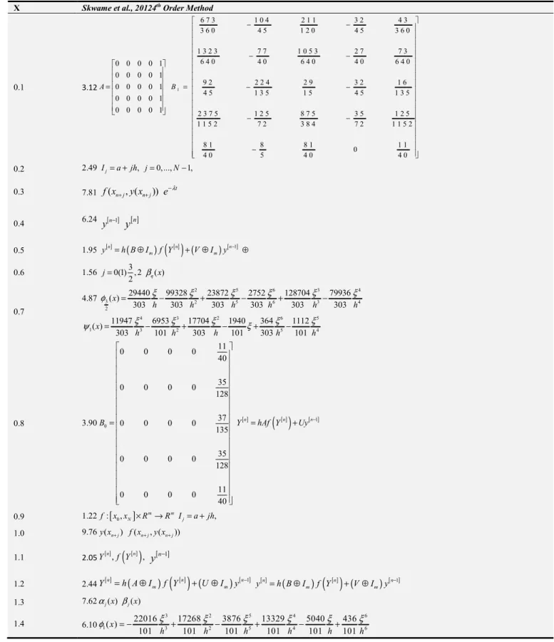
Table 1. Maximum Errors for Example 1.

X Skwame et al., 20124th_{Order Method}

0.1 3.12

0 0 0 0 1 0 0 0 0 1 0 0 0 0 1 0 0 0 0 1 0 0 0 0 1 A

 

 

=

 

 

1

6 7 3 1 0 4 2 1 1 3 2 4 3

3 6 0 4 5 1 2 0 4 5 3 6 0

1 3 2 3 7 7 1 0 5 3 2 7 7 3

6 4 0 4 0 6 4 0 4 0 6 4 0

9 2 2 2 4 2 9 3 2 1 6

4 5 1 3 5 1 5 4 5 1 3 5

2 3 7 5 1 2 5 8 7 5 3 5 1 2 5

1 1 5 2 7 2 3 8 4 7 2 1 1 5 2

8 1 8 8 1 1 1

0

4 0 5 4 0 4 0

 

− −

 

 ₋ ₋ 

 

= _ − − _

 

− −

 

 ₋ 

 

 

B

0.2 2.49 Ij= +a jh, j=0,...,N−1,

0.3 7.81 f x( n j+ , (y xn j+ )) e−λt

0.4 6.24 y[ ]n−1

y

[ ]n

0.5 1.95 y[ ]n h B( Im)f Y

( )

[ ]n (V Im)y[ ]n1

−

= ⊕ + ⊕ ⊕

0.6 1.56 0(1) , 23 2 j= βq( )x

0.7

4.87

2 5 6 3 4

3 2 5 6 3 4

2

29440 99328 23872 2752 128704 79936

( )

303 303 303 303 303 303

x

h h h h h h

ξ ξ ξ ξ ξ ξ

φ = − + − + −

4 3 2 6 5

1 3 2 5 4

11947 6953 17704 1940 364 1112

( )

303 101 303 101 303 101

x

h h h h h

ξ ξ ξ ξ ξ

ψ = − + − ξ+ −

0.8 3.90 0

11

0 0 0 0

40

35

0 0 0 0

128

37

0 0 0 0

135

35

0 0 0 0

128

11

0 0 0 0

40 B

 

 

=_ _

 

 

[ ]n

( )

[ ]n [ ]n1

Y =hAf Y +Uy −

0.9 1.22 :

[

0,

]

m m N

f x x ×R →R Ij= +a jh, 1.0 9.76 (y xn j+) f x( n j+, (y xn j+))

1.1 2.05Y[ ]n,f Y

( )

[ ]n , _y[ ]n−1

1.2 2.44Y[ ]n =h A

(

⊕Im

)

f Y

( )

[ ]n +

(

U⊕Im

)

y[ ]n−1

[ ]n

₍

₎

( )

[ ]n

₍

₎

[ ]n1

m m

y =h B⊕I f Y + V⊕I y − 1.3 7.62αj( )x βj( )x

1.4 6.10

3 2 5 4 6

1 3 2 5 4 6

22016 17268 3876 13329 5040 436

( )

101 101 101 101 101 101

x

h h h h h h

ξ ξ ξ ξ ξ ξ

(8)

X Skwame et al., 20124th_{Order Method}

5 2 3 6 4

2 5 2 3 6 4

4017 60687 40631 475 4365 52203

( )

101 404 202 101 101 404

x

h h h h h h

ξ ξ ξ ξ ξ ξ

φ = − + − + − +

1.5 1.90

0 0 0 0 1 0 0 0 0 1 0 0 0 0 1 0 0 0 0 1 0 0 0 0 1 A

 

 

=

 

 

1

673 104 211 32 43 360 45 120 45 360

1323 77 1053 27 73 640 40 640 40 640

92 224 29 32 16

45 135 15 45 135

2375 125 875 35 125 1152 72 384 72 1152

81 8 81 11

0

40 5 40 40

 

− −

 

 ₋ ₋ 

 

= − − 

 

− −

 

 ₋ 

 

 

B

1.6 1.52 :

[

0,

]

m m

N

f x x ×R →R Ij= +a jh,

1.7 4.76y x( n j+ ) f x( n j+ , (y xn j+ ))

1.8 3.81Y[ ]n,f Y

( )

[ ]n , y[ ]n−1

1.9 1.19Y[ ]n h A

(

Im

)

f Y

( )

[ ]n

(

U Im

)

y[ ]n1

−

= ⊕ + ⊕ [ ]n

(

)

( )

[ ]n

(

)

[ ]n1

m m

y =h B⊕I f Y + V⊕I y −

2.0 _9.52

1 2

0 2

( ) ( ) ( ) ( ) ( )

k

j n j q n q j n j q n q

j j k

−

+ + + +

= = −

 

= + +  + 

 

∑

α_j( )x

X Skwame et al., 2012 6th Order Method

0.1 5.00 0

11

0 0 0 0

40

35

0 0 0 0

128

37

0 0 0 0

135

35

0 0 0 0

128

11

0 0 0 0

40 B

 

 

=_ _

 

 

( ) ( , ),

y x′ = f x y

0.2 1.67 1 b a h

N − =

− k−step

0.3 5.00λ

Y

₁[ ]n

,

Y

₂[ ]n

, ...,

Y

_s[ ]n

0.4 3.00 [ ] [ ]

[ ]

[ ] 1

2

. . .

n

n s Y Y

Y

          =_ _        

[ ]

( )

[ ]

( )

[ ]

( )

[ ]

( )

1

2

.

n

n s f Y

f Y

 

 

= 

 

 

0.5 1.50Y[ ]n =hAf Y

( )

[ ]n +Uy[ ]n−1 y[ ]n =hBf Y

( )

[ ]n +Vy[ ]n−1

0.6 5.00αq( )x a q

(9)

X Skwame et al., 2012 6th Order Method

0.7 1.50

4 2 3 6 5

2 3 2 5 4

7359 8167 5584 1155 142 1166

( )

202 202 101 101 101 101

x

h h h h h

ξ ξ ξ ξ ξ

ψ = − + + ξ− + 3 2 34 65 32 54

2

704 64 704 32 336 80

( )

303 101 303 303 101 101

x

h h h h h

ξ ξ ξ ξ ξ

ψ = − ξ+ + − −

0.8 9.00Y[ ]n =hAf Y

( )

[ ]n +Uy[ ]n−1

( )

(

)

1

M z = +V zB I−zA−U

0.9 4.50 j=0,...,N−1,

1 b a h

N − =

−

1.0 1.50 t

e−λ

λ

1.1 4.50y[ ]n [ ] [ ]

[ ]

[ ] 1

2 .

.

n

n s Y Y

Y

 

 

=_ _

 

 

1.2 2.70⊕Y[ ]n =hAf Y

( )

[ ]n +Uy[ ]n−1 1.3 1.35 0(1) , 23

2

j= βq( )x

1.4 4.50

2 5 6 3 4

3 2 5 6 3 4

2

29440 99328 23872 2752 128704 79936 ( )

303 303 303 303 303 303

x

h h h h h h

ξ ξ ξ ξ ξ ξ

φ = − + − + − 1 43 23 2 65 45

11947 6953 17704 1940 364 1112 ( )

303 101 303 101 303 101

x

h h h h h

ξ ξ ξ ξ ξ

ψ = − + − ξ+ −

1.5 1.35 0

11

0 0 0 0

40

35

0 0 0 0

128

37

0 0 0 0

135

35

0 0 0 0

128

11

0 0 0 0

40 B

 

 

=_ _

 

 

( , )w z det(wI M z( ))

Φ = −

1.6 8.10 j=0,...,N−1,

1

b a h

N

− =

−

1.7 4.05 t

e−λ λ

1.8 1.35

_y

[ ]n [ ]

[ ] [ ]

[ ]

1 2

.

n n

n

n s

Y





















=

_

_

















1.9 4.05

⊕

Y[ ]n =hAf Y

( )

[ ]n +Uy[ ]n−1 2.0 2.43βj( )x

3 0(1) , 2

2 j=

X FETR

0.1 1.5576y a( )=y0I=

[

x x0, N

]

0.2 1.7321

0 0

( )

k k

j n j j n j

j j

y h x f

α + β +

= =

 

=  

 

(10)

X FETR

0.3 1.1797 f Y

( )

₁[ ]n ,f Y

( )

₂[ ]n ,...,f Y

( )

s[ ]n [ ] [ ] [ ]

1 1 1

1 , 2 ,...,

n n n

r

Y − Y − Y −

0.4 3.8528 [ ]

[ ] [ ] [ ] 1 1 1 2 1 1 . . . n n n n r y y y y − − − −           =_ _         [ ] [ ] [ ] [ ] 1 2

.

n n n n r

y





















=

_

_

















0.5 4.1553M A U B V   =    1 2 0 2 ( ) ( ) ( ) ( ) ( ) k

j n j q n q j n j q n q

j j k

− + + + + = = −   = + +  +   

∑

0.6 2.17002 1, 1, 2 2

r r

+ ₌ 2 3 4 5 6

0 2 3 4 5 6

1225 8035 3419 3187 193 19

( ) 1

303 1212 606 1212 303 303

x

h h h h h h

ξ ξ ξ ξ ξ ξ

φ = − + − + − +

0.7 1.8980

0 0 0 0 0 0 0 0 0 1

101 388 231 4 97 5888 35

0 0 0

5040 1008 1008 315 112 3024 432

159 303 387 3 4023 891 11

0 0 0

112 56 244 56 448 112 448

113 530 256 101 68864 152

0 0 0

633 1477 4431 13293 39879 211

75 675 15

0 0 0

404 808 101

366 738 192

0 0 0

101 101 101

− − − − − − − − − − − − − − − − 257 39879

675 225 325 9

1616 101 404 1616

2187 3584 1485 13

101 101 101 101

366 738 192 2187 3584 1485 13

0 0 0

101 101 101 101 101 101 101

113 530 256 101 6

0 0 0

633 1477 4431 13293

159 303 387 3

0 0

112 56 244 56

101 388 231 4

0 0

5040 1008 1008 315

− − − − − − − − − − − − − −

8864 152 257 39879 211 39879

4023 891 11

0

448 112 448

97 5888 35

0

112 3024 432

                                                                       ₋ ₋          − −          ₋ ₋       

1 0 0 0 0 0 1 0 0 0 0 0 1 0 0 0 0 0 1 0 0 0 0 0 1 I         =        

0.8 5.1155y x′( )= f x y( , ), y a( )=y₀

0.9 4.4037

k

−

step

0 0

( )

k k

j n j j n j

j j

y h x f

α + β +

= =

 

=  

 

∑

1.0 2.1834Y₁[ ]n,Y₂[ ]n,...,Ys[ ]n [ ]

( )

[ ]

( )

[ ]

1 , 2 ,...,

n n n

s

f Y f Y f Y

1.1 4.6956

( )

[ ]

(11)

X FETR

1.2 1.5467

y

[ ]n

=

hBf Y

( )

[ ]n

+

Vy

[ ]n−1 M A U

B V

 

= 

 

1.3 6.8444

α

_q

( )

x

q a b

=

1.4 1.6501

4 2 3 6 5

2 3 2 5 4

7359 8167 5584 1155 142 1166

( )

202 202 101 101 101 101

x

h h h h h

ξ ξ ξ ξ ξ

ψ = − + + ξ− +

2 4 6 3 5

3 3 5 2 4

2

704 64 704 32 336 80

( )

303 101 303 303 101 101

x

h h h h h

ξ ξ ξ ξ ξ

ψ = − ξ+ + − −

1.5 1.7794y x′( )= f x y( , ), y a( )=y0

1.6 2.0002k−step

0 0

( )

k k

j n j j n j

j j

y h x f

α + β +

= =

 

=  

 

∑

1.7 1.4414Y₁[ ]n,Y₂[ ]n,...,Y_s[ ]n

( )

1[ ] ,

( )

2[ ] ,...,

( )

[ ]

n n n

s

f Y f Y f Y

1.8 8.5234

( )

[ ]

( )

[ ]

( )

[ ]

( )

1 2

. . .

n

n s

f Y f Y f Y

f Y

 

 

= 

 

 

[ ] [ ]

[ ]

[ ] 1 1

1 2

1

1 .

.

n

n r y y

y

−

 

 

=_ _

 

 

1.9 2.6913y[ ]n =hBf Y

( )

[ ]n +Vy[ ]n−1 M A U

B V

 

= 

 

2.0 5.8666

β

_q

( )

x

α

_q

( )

x

X SETR

0.1 8.9860 :

[

₀,

]

m N

y x x →R :

[

₀,

]

m m

N

f x x ×R →R

0.2 3.5800

f

_{n j}₊

y x

(

_{n j}₊

)

0.3 2.2793

Y

₁[ ]n

,

Y

₂[ ]n

,...,

Y

_r[ ]n Y[ ]n,f Y

( )

[ ]n , 0.4 2.3103 [ ] [ ] [ ]

1

,

2

,...,

n n n s

Y

[ ]n

(

)

( )

[ ]n

(

)

[ ]n1

m m

Y =h A⊕I f Y + U⊕I y − 0.5 9.6111αj( )x βj( )x

0.6 3.5877

3 2 5 4 6

1 3 2 5 4 6

22016 17268 3876 13329 5040 436 ( )

101 101 101 101 101 101

x

h h h h h h

ξ ξ ξ ξ ξ ξ

φ = − + − + − + 2 55 22 33 66 44

4017 60687 40631 475 4365 52203

( )

101 404 202 101 101 404

x

h h h h h h

ξ ξ ξ ξ ξ ξ

φ = − + − + − +

0.7 1.3030

0 0 0 0 1 0 0 0 0 1 0 0 0 0 1 0 0 0 0 1 0 0 0 0 1 A

 

 

=

 

 

1

673 104 211 32 43

360 45 120 45 360

1323 77 1053 27 73

640 40 640 40 640

92 224 29 32 16

45 135 15 45 135

2375 125 875 35 125

1152 72 384 72 1152

81 8 81 11

0

40 5 40 40

B

 

− −

 

 − − 

 

=_ − − _

 

− −

 

 ₋ 

 

 

0.8 4.9168I=

[

x x₀, _N

]

y:

[

x x₀, N

]

→Rm

0.9 1.6269

y

_{n j}₊ fn j+

1.0 1.2028Y₁[ ]n−1,Y₂[ ]n−1,...,Y_r[ ]n−1 1[ ], 2[ ],..., [ ]

n n n

r

(12)

X SETR

1.1 4.4549 [ ]

[ ]

1 2

.

n n

n

n r

y





















=

_

_

















[ ] [ ] [ ] 1

,

2

,...,

n n n s

Y

1.2 1.6290M z

( )

= +V zB I

(

−zA

)

−1U

1 2

0 2

( ) ( ) ( ) ( ) ( )

k

j n j q n q j n j q n q

j j k

−

+ + + +

= = −

 

= + +  + 

 

∑

1.3 6.06452 1, 1, 2 2

r r

+ ₌ 2 3 4 5 6

0 2 3 4 5 6

1225 8035 3419 3187 193 19

( ) 1

303 1212 606 1212 303 303

x

h h h h h h

ξ ξ ξ ξ ξ ξ

φ = − + − + − +

1.4 2.1259

0 0 0 0 0 0 0 0 0 1

101 388 231 4 97 5888 35

0 0 0

5040 1008 1008 315 112 3024 432

159 303 387 3 4023 891 11

0 0 0

112 56 244 56 448 112 448

113 530 256 101 68864 152

0 0 0

633 1477 4431 13293 39879 211

75 675 15

0 0 0

404 808 101

366 738 192

0 0 0

101 101 101

− − − − −

− − − −

−

257 39879

675 225 325 9

1616 101 404 1616

2187 3584 1485 13

101 101 101 101

366 738 192 2187 3584 1485 13

0 0 0

101 101 101 101 101 101 101

113 530 256 101 6

0 0 0

633 1477 4431 13293

159 303 387 3

0 0

112 56 244 56

101 388 231 4

0 0

5040 1008 1008 315

− − −

−

− −

− − −

8864 152 257 39879 211 39879

4023 891 11

0

448 112 448

97 5888 35

0

112 3024 432

 

 

 ₋ ₋ 

 

− −

 

 ₋ ₋ 

 

 

1 0 0 0 0 0 1 0 0 0 0 0 1 0 0 0 0 0 1 0 0 0 0 0 1 I

 

 

=

 

 

1.5 1.1312

I

=

[

x x

₀

,

N

]

:

[

0,

]

m N

y x x →R

1.6 4.1787

y

_{n j}₊ fn j+

1.7 1.5316Y₁[ ]n−1,Y₂[ ]n−1,...,Y_r[ ]n−1 Y₁[ ]n,Y₂[ ]n,...,Yr[ ]n

1.8 5.6758 [ ]

[ ]

1

2 . . .

n

n r y y

y

 

 

=_ _

 

 

[ ] [ ] [ ]

1 , 2 ,...,

n n n

s

Y Y Y

1.9 2.0273M z

( )

= +V zB I

(

−zA

)

−1U Φ( , )w z =det(wI−M z( )). 2.0 9.4748q a

b

= 2 1

, 1, 2 2 r

r

(13)

Problem 2

2 3 4 5 6

0 ₂ ₃ ₄ ₅ ₆

1225 8035 3419 3187 193 19

( ) 1

303 1212 606 1212 303 303

x

h h h h h h

ξ ξ ξ ξ ξ ξ

φ = − + − + − +

,

3 2 5 4 6

1 ₃ ₂ ₅ ₄ ₆

22016 17268 3876 13329 5040 436

( )

101 101 101 101 101 101

x

h

h h h h h

ξ ξ ξ ξ ξ ξ

φ = − + − + − +

,

5 2 3 6 4

2 5 2 3 6 4

4017 60687 40631 475 4365 52203

( )

101 404 202 101 101 404

x

h

h h h h h

ξ ξ ξ ξ ξ ξ

φ = − + − + − +

,

2 5 6 3 4

3 ₂ ₅ ₆ ₃ ₄

2

29440 99328 23872 2752 128704 79936

( )

303 303 303 303 303 303

x

h h h h h h

ξ ξ ξ ξ ξ ξ

φ = − + − + −

Exact Solution

4 3 2 6 5

1 ₃ ₂ ₅ ₄

11947 6953 17704 1940 364 1112 ( )

303 101 303 101 303 101

x

h

h h h h

ξ ξ ξ ξ ξ

ψ = − + − ξ+ −

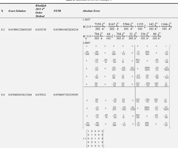
Table 2. Maximum Errors for Example 1.

X Exact Solution

Khadijah 2015 4th

Order Method

FETR Absolute Error

0.2 0.019801326693245 0.818738 0.0198014832636218 1.5657

4 2 3 6 5

2 3 2 5 4

7359 8167 5584 1155 142 1166

( )

202 202 101 101 101 101

x

h h h h h

ξ ξ ξ ξ ξ

ψ = − + + ξ− +

2 4 6 3 5

3 3 5 2 4

2

704 64 704 32 336 80

( )

303 101 303 303 101 101

x

h h h h h

ξ ξ ξ ξ ξ

ψ = − ξ+ + − −

0.4 0.076883653613364 0.670321 0.0768857343339293 2.0807

0 0 0 0 0 0 0 0 0 1

101 388 231 4 97 5888 35

0 0 0

5040 1008 1008 315 112 3024 432

159 303 387 3 4023 891 11

0 0 0

112 56 244 56 448 112 448

113 530 256 101 68864 152

0 0 0

633 1477 4431 13293 39879 211

75 675 15

0 0 0

404 808 101

366 738 192

0 0 0

101 101 101

− − − − −

− − − −

−

257 39879

675 225 325 9

1616 101 404 1616

2187 3584 1485 13

101 101 101 101

366 738 192 2187 3584 1485 13

0 0 0

101 101 101 101 101 101 101

113 530 256 101 6

0 0 0

633 1477 4431 13293

159 303 387 3

0 0

112 56 244 56

101 388 231 4

0 0

5040 1008 1008 315

− − −

−

− −

− − −

8864 152 257 39879 211 39879

4023 891 11

0

448 112 448

97 5888 35

0

112 3024 432

 

 

 ₋ ₋ 

 

− −

 

 ₋ ₋ 

 

 

1 0 0 0 0 0 1 0 0 0 0 0 1 0 0 0 0 0 1 0 0 0 0 0 1 I

 

 

=_ _

 

(14)

X Exact Solution

Khadijah 2015 4th

Order Method

FETR Absolute Error

0.6 0.164729788588728 0.545813 0.164732324486997

1.2061

0 0 0 0 1 0 0 0 0 1 0 0 0 0 1 0 0 0 0 1 0 0 0 0 1 A

 

 

=

 

  1

673 104 211 32 43

360 45 120 45 360

1323 77 1053 27 73

640 40 640 40 640

92 224 29 32 16

45 135 15 45 135

2375 125 875 35 125 1152 72 384 72 1152

81 8 81 11

0

40 5 40 40

B

 ₋ ₋ 

 

 − − 

 

=_ − − _

 

− −

 

 ₋ 

 

 

0.8 0.273850962926309 0.449325 0.273853652953028

2.6900

0

11

0 0 0 0

40 35

0 0 0 0

128 37

0 0 0 0

135 35

0 0 0 0

128 11

0 0 0 0

40

B

 

 

=_ _

 

 

( , )w z det(wI M z( )).

Φ = −

1.0 0.393469340287367 0.367873 0.393473662912352 4.3226Φ( , )w z =det(wI−M z( )) Φ( , )w z =det(wI−M z( ))

5. Conclusion

We derived block Extended Trapezoidal Rule of First (ETRs) that are A-stable of up to order 8. The methods were shown tocompete favorablythan other existing methodsin terms of accuracy (see tables 1 and 2). Our newly derived methods in block form are shown to have extensive regions of stability and in particular are A-stable up to order 8 and so very suitable for stiff system of ordinary differential equations. The continuous formulation for each step number kis evaluated at the end point of the interval to recover the individual main method for FETR, SETR and EETR in (13) and their counterparts schemes in (8), (11) and (12) respectively, to this end, the idea of additional conditions is discarded. Furthermore, we do not need any pair in our implementation. Our block methods preserve the A-stability property of the trapezoidal rule (refer to figure 1), they are also less expensive in terms of the number of functions evaluation per step.

References

[1] Awari, Y. S. (2017). A-Stable Block ETRs/ETR2s Methods for Stiff ODEs, MAYFEB Journal of Mathematics Vol. 4: Pages 33-52.

[2] Awari, Y. S., Garba, E. J. D., Kumleng, M. G. and Tsaku, N. (2016). Efficient implementation of Some Block Extended Trapezoidal rule of first kind (ETRs) class of method Applied to First Order Initial Value Problems of Differential Equations, Global Journal of Mathematics, Vol. 7 (2).

[3] Biala, T. A., Jator, S. N., Adeniyi, R. B. and Ndukum, P. L. (2015). Block Hybrid Simpson’s Method with Two Off-grid Points for Stiff Systems International Journal of Nonlinear Science Vol. 20 (1), pp. 3-10.

[4] Happy K., Shelly, Arora and Nagaich, R. K. (2013). Solution of Non Linear Singular Perturbation Equation Using Hermite Collocation Method, Applied Mathematical Sciences, Vol. 7, 2013, no. 109, 5397–5408.

[5] Khadijah, M. Abualnaja, (2015). A Block Procedure with Linear Multistep Methods Using Legendre Polynomials for Solving ODEs, Applied Mathematics 6:717-723.

[6] Miletics, E. and Moln´arka, G. (2009). Taylor Series Method with Numerical Derivatives for Numerical Solution of ODE Initial Value Problems, HU ISSN 1418-7108: HEJ Manuscript no.: ANM-030110-B.

[7] Okuonghae, R. I. andIkhile, M. N. O. (2011). A(α)-Stable Linear Multistep Methods. for Stiff IVPs in ODEs Acta Univ. Palacki. Olomuc., Fac. rer. nat., Mathematica 50 (1), 73–90. [8] Skwame, Y., Sunday, J., Ibijola, E. A. (2012). L-Stable Block

Hybrid Simpson’s Methods for Numerical Solution of Initial Value Problems in Stiff Ordinary Differential Equations, International Journal of Pure and Applied Sciences and Technology 11(2):45-54.

[9] Tahmasbi, A. (2008). Numerical Solutions for Stiff Ordinary Differential Equation Systems, International Mathematical Forum, 3, 2008, no. 15, 703 – 711.