J. C. F. Pereira and A. Sequeira (Eds) Lisbon, Portugal,14-17 June 2010
HIGH ORDER NUMERICAL SIMULATION OF FLUID-STRUCTURE INTERACTION IN HUMAN PHONATION
Martin Larsson and Bernhard M¨uller Norwegian University of Science and Technology
Department of Energy and Process Engineering, 7491 Trondheim, Norway e-mail: {martin.larsson,bernhard.muller}@ntnu.no
Key words: Fluid-Structure Interaction, High Order Method, Finite Difference, Phona-tion
Abstract. Fluid-structure interaction in a simplified two-dimensional model of the larynx is considered in order to study human phonation. The flow is driven by an imposed pressure gradient across the glottis and interacts with the moving vocal folds in a self-sustained oscillation. The flow is computed by solving the 2D compressible Navier–Stokes equations using a high order finite difference method, which has been constructed to be strictly stable for linear hyperbolic and parabolic problems. The motion of the vocal folds is obtained by integrating the linear elastic wave equation using a similar high order difference method as for the flow equations. Fluid and structure interact in a two-way coupling. In each time step at the fluid-structure interface, the structure provides the fluid with new no-slip boundary conditions and new grid velocities, and the fluid provides the structure with new traction boundary conditions which are imposed via the simultaneous approximation term (SAT) approach.
1 INTRODUCTION
Fluid-structure interaction (FSI) occurs when a flexible structure interacts with a fluid. The fluid flow exerts a stress on the structure which causes it to deform, thereby generating a new geometry for the fluid flow. A direct consequence of FSI in the vocal tract is voice generation, where the motion of the soft tissue of the vocal folds interacts dynamically with the glottal airflow to produce sound. The self-sustained oscillations of the vocal folds can be explained by the Bernoulli principle which states that in the absence of gravity for inviscid incompressible steady flow, the velocity v, pressure p and density ρ are related byp+ρv2/2 = const. The vocal folds being closed in their equilibrium position, initially at rest, are forced apart by the increasing lung pressure. As the air starts flowing, the velocity in the glottis increases and thus the pressure must decrease according to the Bernoulli principle. The pressure drop together with restoring elastic forces results in a closure of the vocal folds and a build-up of pressure. This cycle then repeats itself, driven only by the lung pressure. The computational challenge in aeroelastic simulations lies in dealing with unsteady flows at high Reynolds numbers, large deformations, moving interfaces, fluid-structure interaction and intrinsically 3D motion [3].
In this paper, we employ a high order finite difference approach based on summation by parts (SBP) operators [16, 5, 4] to solve the compressible Navier–Stokes equations and the linear elastic wave equation on first order form. Fluid and structure interact in a two-way coupling, meaning that fluid stresses deform the flexible structure which in turn causes the fluid to conform to the new structural boundary via boundary conditions. The approach has been tested for a 2D model of the larynx and the vocal folds.
2 GOVERNING EQUATIONS
2.1 Compressible Navier–Stokes equations
The perturbation formulation is used to minimize cancellation errors when discretizing the Navier–Stokes equations for compressible low Mach number flow [15, 12]. The 2D compressible Navier–Stokes equations in conservative form can be expressed in perturba-tion form as [13, 8] U0t + Fc 0 x+G c0 y = F v0 x+G v0 y, (1)
where the vector U0 denotes the perturbation of the conservative variables with respect to the stagnation values. U0 and the inviscid (superscript c) and viscous (superscript v) flux vectors are e.g. defined in [8].
General moving geometries are treated by a time dependent coordinate transformation τ =t,ξ =ξ(t, x, y),η=η(t, x, y). The transformed 2D conservative compressible Navier– Stokes equations in perturbation form read [8]
ˆ Uτ0 + ˆFξ0+ ˆG0η = 0, (2) where Uˆ0 = J−1U0, Fˆ0 = J−1(ξ tU0 +ξx(Fc0 −Fv0) + ξy(Gc0 −Gv0)) and Gˆ0 = J−1(η tU0+ηx(Fc0−Fv0) + ηy(Gc0−Gv0)).
No-slip adiabatic wall boundary conditions and the Navier–Stokes Characteristic Bound-ary Conditions (NSCBC) technique by Poinsot and Lele in [14] are employed at the outflow [9]. At the inflow, pressure, temperature and velocity in the y-direction are imposed as p=patm+ ∆p, T =T0 = 310 K, andv = 0, respectively.
2.2 Linear elastic wave equation
The 2D linear elastic wave equation written as a first order hyperbolic system reads in Cartesian coordinates
qt=Aqx+Bqy, (3) where the unknown vector q = (u, v, f, g, h)T contains the velocity components u, v and the stress componentsf, g, hand the coefficient matricesA,B (cf. e.g. [2, 11, 10]) depend on the the Lam´e parametersλ, µand the densityρwhich are here all taken to be constant in space and time.
The linear combinationP(kx, ky) =kxA+kyBcan be diagonalized with real eigenvalues and linearly independent eigenvectors. The eigenvalue matrix is defined as the diagonal matrix with the eigenvalues of P(kx, ky) in decreasing order,
˜ Λ(kx, ky) = (k2x+k 2 y) 1/2diag(c p, cs,0,−cs,−cp) = diag n ˜ λi(kx, ky) o5 i=1 , (4) where the wave speeds arecp =
p
(λ+ 2µ)/ρ andcs =
p
µ/ρ, referred to as primary and secondary (or shear) wave velocity, respectively.
To treat curvilinear grids we introduce the mapping x = x(ξ, η), y = y(ξ, η). The Jacobian determinant J of the transformation is given by J−1 = xξyη −xηyξ and the linear elastic wave equation can then be written as
ˆ
qt= ( ˆAˆq)ξ+ ( ˆBq)ˆη (5) where the hats signify that the quantities are in transformed coordinates, i.e. ˆq = J−1q,
ˆ
A=ξxA+ξyB and ˆB =ηxA+ηyB. 2.3 Characteristic variables
In order to describe the SAT expressions in transformed coordinates we need to find the characteristic variables for the transformed equation in which the coefficient matrices are linear combinations of the coefficient matrices in the x- and y-directions.
ˆ
qt= ((kxA+kyB)ˆq)k (6) where k = ξ, η. We form the linear combination P(kx, ky) =kxA+kyB. The coefficient matrices A and B have the same set of eigenvalues Λ = diag(cp, cs,0,−cs,−cp), whereas for the linear combinationP(kx, ky) we get ˜Λ(kx, ky) = (k2x+k2y)1/2Λ. To find the linearly
independent eigenvectors of P(kx, ky), we solve the underdetermined system (P(kx, ky)− ˜
λiI)vi = 0 for i= 1, ...,5. These five eigenvectorsvi become the columns in the matrix
T(kx, ky) = kxc˜p/λ −ky/k¯ 0 −ky/¯k −kxc˜p/λ kycp/λ˜ kx/k¯ 0 kx/k¯ −ky˜cp/λ k2 xα+ky2 −2kxky˜csρ/(¯kr2) ky2 2kxky˜csρ/(¯kr2) kx2α+ky2 2kxkyµ/λ ρ˜cs −kxky −ρ˜cs 2µkxky/λ k2 yα+kx2 2kxky˜csρ/(¯kr2) kx2 −2kxky˜csρ/(¯kr2) ky2α+kx2 (7)
We have some degrees of freedom in choosing T, because each column can be scaled by any nonzero constant. The inverse of this matrix is obtained with a symbolic computer program, the result being
T−1(kx, ky) = 1 2r2 kxλ ˜ cp kyλ ˜ cp k2x αr2 2 kykx αr2 k2 y αr2 −ky¯k kx¯k − ¯ kkxky ρ˜cs ¯ k2r2 ρ˜cs ¯ kkxky ρ˜cs 0 0 −2¯k α + 4k2 y βr2 −8 kxky(λ+µ) r2(λ+ 2µ) 2¯k α + 4 k2x βr2 −ky¯k kx¯k ¯ kkxky ρ˜cs −¯k 2r2 ρ˜cs −kk¯ xky ρ˜cs −λkx ˜ cp − λky ˜ cp k2 x αr2 2 kykx αr2 k2y αr2 (8)
where the parameters are defined by ¯k = (kx2−k2y)/(k2x+ky2), r = (kx2+ky2)1/2, ˜cp =rcp, ˜
cs = rcs, α = (λ + 2µ)/λ and β = αλ/µ. For all directions (kx, ky) we have that T−1(k
x, ky)P(kx, ky)T(kx, ky) = ˜Λ(kx, ky). The transformation to characteristic variables u is given by u(k) = T−1(kx, ky)ˆq for each of the two coordinate directions k = ξ, η. The transformation back to flow variables is given by ˆq =T(kx, ky)u(k).
3 STRICTLY STABLE HIGH ORDER DIFFERENCE METHOD
3.1 Energy method
The energy method is a general technique to prove sufficient conditions for well-posedness of partial differential equations (PDE) and stability of difference methods with general boundary conditions.
Consider the solution of the model problem in 1D with
ut=λux, λ >0, 0≤x≤1, t≥0, u(x,0) =f(x), u(1, t) = g(t). (9) The symbol λ represents here a general eigenvalue for the hyperbolic system and should not be confused with the Lam´e parameter. Define theL2 scalar product for real functions
v and w on the interval 0≤x≤1 as (v, w) =
Z 1
0
v(x)w(x)dx (10)
which defines a norm of the continuous solution at some time t and an energy E(t) =
||u(·, t)||2 = (u, u). Using integration by parts (v, w
x) = v(1, t)w(1, t)−v(0, t)w(0, t)− (vx, w), we get dEdt = d
||u||2
dt = (ut, u) + (u, ut) = λ[(ux, u) + (u, ux)] = λ[(ux, u) + [u 2]1
0− (ux, u)] =λ[u2(1, t)−u2(0, t)]. If λ >0, the boundary condition u(1, t) = 0 yields a non-growing solution (note that periodic boundary conditions would also yield a non-non-growing solution), i.e. E(t) ≤ E(0) = ||f(x)||2. Thus, the energy of the solution is bounded by the energy of the initial data. Hence the problem is well-posed.
3.2 Summation by parts operators
The idea behind the summation by parts technique (cf. e.g. [4]) is to use an operator Q which satisfies the corresponding discrete property as the integration by parts of the continuous function, called the summation by parts (SBP) property. For the numerical so-lution of (9), we introduce the equidistant gridxj =jh,j = 0, ..., N,h= 1/N, and a solu-tion vector containing the solusolu-tion at the discrete grid points,u= (u0(t), u1(t), ..., uN(t))T. The semi-discrete problem can be stated using a difference operator Qapproximating the first derivative,
du
dt =λQu, ui(0) = f(xi). (11) We also define a discrete scalar product and corresponding norm and energy by
(u,v)h =h
X
i,j
hijuivj =huTHv, Eh(t) =||u||2h = (u,u)h, (12) where the symmetric and positive definite norm matrixH = diag(HL, I, HR) has compo-nents hij. In order for (12) to define a scalar product, HL and HR must be symmetric and positive definite. We say that the scalar product satisfies the summation by parts property (SBP), if
(u, Qv)h =uNvN −u0v0−(Qu,v)h. (13) It can be seen that this property is satisfied if the matrix G=HQ satisfies the condition that G+GT = diag(−1,0, ...,0,1). IfQand its corresponding norm matrix H satisfy the SBP property (13), then the energy method for the discrete problem yields:
dEh dt =
d||u||2 h
dt = (ut, u)h+ (u, ut)h =λ[(Qu, u)h+ (u, Qu)h] (14) = λ[(Qu, u)h+u2N −u
2
0−(Qu, u)h] =λ[u2N −u 2
0]. (15)
For diagonal HL andHRthere exist difference operatorsQaccurate to order O(h2s) in the interior andO(hs) near the boundaries for s= 1,2,3 and 4. These operators have an effective order of accuracy O(hs+1) in the entire domain. Explicit forms of such operators Q and norm matrices H were derived by Strand [16].
For this study, we use an SBP operator based on the central sixth order explicit finite difference operator (s= 3) which has been modified near the boundaries in order to satisfy the SBP property giving an effective O(h4) order of accuracy in the whole domain. 3.3 Simultaneous approximation term
Since one of the terms in (15) is non-negative, strict stability does not follow when us-ing the injection method for the summation by parts operator, i.e. by usus-ing uN(t) =g(t). In contrast, the simultaneous approximation term (SAT) method is an approach where a linear combination of the boundary condition and the differential equation is solved at the boundary. This leads to a weak imposition of the physical boundary conditions. The imposition of SAT boundary conditions is accomplished by adding a source term to the difference operator, proportional to the difference between the value of the discrete solu-tionuN and the boundary condition to be fulfilled. The SAT method for the semidiscrete advection equation (11) can be expressed as
du
dt =λQu−λτS(uN −g(t)) where S=h−1H−1(0,0, ...,0,1)T and τ is a free parameter.
The added term does not alter the accuracy of the scheme since it vanishes when the analytical solution is substituted. Thus, we can imagine the SAT expression as a modification to the difference operator so that we are effectively solving an equation ut =λQu˜ with ˜Q=Q+Qsat without imposing the boundary conditions directly. When H is diagonal, the scheme is only modified at one point on the boundary. We can now show that this scheme is strictly stable for g(t) = 0. The energy rate for the solution of the semi-discrete equation is dEh
dt = d||u||2
h
dt = (ut,u)h + (u,ut)h = λ[(u, Qu−τSuN)h + (Qu−τSuN,u)h] =λ[(u, Qu)h−τ(u,S)huN+(Qu,u)h−τ(S,u)huN] = λ[(1−2τ)u2N−u20] since (S,u)h = (u,S)h = huTHh−1H−1(0,0, ...,0,1)T = uN. The discretization is time stable if τ ≥1/2.
The extension to hyperbolic systems (cf. [1]) of the strictly stable SAT method for hyperbolic systems ut = Λux in one space dimension with diagonal coefficient matrices (r unknowns and r equations) is done in the following way. The coefficient matrix Λ is chosen such that the eigenvalues are in descending order, i.e. λ1 > λ2 > ... > λk > 0 > λk+1 > ... > λr. The solution vector is split into two parts corresponding to positive and negative eigenvalues uI = (u(1), ..., u(k))T and uII = (u(k+1), ..., u(r))T, where u(i) is the eigenvector, i.e. the characteristic variable corresponding to the eigenvalue λ(i). We define uI = (u(1), ...,u(k))T and uII = (u(k+1), ...,u(r))T, where the components u(i) are grid functions of lengthN + 1.
For the components in uI we have boundary conditions at x= 1, and for uII we need to specify boundary conditions at x= 0, as this is required for well-posedness.
Since we are here dealing with characteristic variables, we need to transform our phys-ical boundary conditions to boundary conditions for the characteristic variables. This is done by the boundary functions gI(t) = (g(1)(t), ..., g(k)(t)), gII(t) = (g(k+1)(t), ..., g(r)(t)) and the coupling matrices R and L defined by
uI(1, t) =RuII(1, t) +gI(t), uII(0, t) =LuI(0, t) +gII(t). (16) The SAT method is then:
du(i) dt = λiQu (i)−λ iτS(i)(u (i) N −(RuII) (i) N −g(i)(t)), 1≤i≤k du(i) dt = λiQu (i)+λ iτS(i)(u (i) 0 −(LuI) (i−k) 0 −g(i)(t)), k+ 1≤i≤r (17)
whereS(i) =h−1H−1(0,0, ...,1)T for 1≤i≤k and S(i)=h−1H−1(1,0, ...,0)T fork+ 1≤
i ≤ r. Regarding the notation, (RuII)(i)N should be interpreted as follows: uII is an (r−k)×1 vector where each component is a grid function of length N+ 1. MultiplyingR (being ak×(r−k) matrix) withuIIyields a new vector of grid functions (k×1 vector). Take the (i)th grid function in this vector and finally the Nth component in the resulting grid function. As shown in [1], the SAT method is both stable and time stable provided that 1−p 1− |R||L| |R||L| ≤τ ≤ 1 +p1− |R||L| |R||L| (18)
with the additional constraint that |R||L| ≤ 1, where the matrix norm is defined as
|R|=ρ(RTR)1/2 and ρis the spectral radius.
4 SAT EXPRESSIONS FOR THE LINEAR ELASTIC WAVE EQUATION
Notation for boundary conditions
We adopt the notation u(k0, t) = ¯u(k = k0, t) to represent a 1D boundary condition on the solution variable u in any direction k where k = x or k = y and ¯u(k, t) is the given functions of time on the boundaries k = 0 and k = 1 which the solution variable u should match on those boundaries. For example, ¯u(x = 1, t) is the given u-velocity at the boundary x = 1 and u(1, t) is the corresponding solution to the equations. In 2D, the boundary condition also dependends on the second coordinate direction, which we indicate by ¯u(x = 1, y, t) and ¯u(x, y = 1, t) for boundary conditions in the x- and y-direction, respectively. Finally, for the discretized 2D boundary conditions, we write instead ¯uj(x= 1, t) = ¯u(x= 1, yj, t) and ¯ui(y= 1, t) = ¯u(xi, y = 1, t).
4.1 Presentation of SAT expressions
SAT expressions for the linear elastic wave equation were derived in [10], here we summarize the findings.
The characteristic variables are u(kx, ky) = T−1(kx, ky)ˆq where ˆq = J−1(u, v, f, g, h)T We form the two sub-vectors corresponding to positive and negative eigenvalues as
uI(kx, ky) = (u1, u2)T, uII(kx, ky) = (u4, u5)T (19) with the aim to form boundary conditions with the matrices R and L. Since many components inT−1(k
x, ky) occur in positive/negative pairs, it is easy to find 2×2 matrices L and R which, when applied to uI,II(kx, ky) in Eq. (16), isolate the components which we need in order to state the boundary conditions. Eq. (16) now gives our new boundary functions gI(k
x, ky, t) andgII(kx, ky, t) as
gI(kx, ky, t) = ¯uI(kx, ky, k= 0, t)−R¯uII(kx, ky, k= 0, t) (20) gII(kx, ky, t) = ¯uII(kx, ky, k = 1, t)−L¯uI(kx, ky, k= 1, t) (21) where the functions ¯uI,II(kx, ky, k, t) are the previously defineduI,II(kx, ky) from Eq. (19) but with the solution variables substituted for their corresponding time-dependent bound-ary conditions. Note that L and R are independent of the direction, but depend on the particular type of boundary condition to impose (velocity or traction). For boundary con-ditions on the velocities u and v, we get using the definitions (20)–(21) and choosing L and Rso that the appropriate components of the characteristic variables uare recovered, the following expressions
gI(kx, ky, t) = J −1 r2 λ ˜ cp (kxu(k¯ = 1, t) +kyv(k¯ = 1, t)) ¯ k(−kyu(k¯ = 1, t) +kx¯v(k= 1, t)) , R = 0 1 −1 0 (22) gII(kx, ky, t) = J−1 r2 ¯ k(−kyu(k¯ = 0, t) +kxv(k¯ = 0, t)) λ ˜ cp (−kxu(k¯ = 0, t)−kyv(k¯ = 0, t)) , L= 0 −1 1 0 (23) where ¯u(k, t),v(k, t) are the given boundary conditions on¯ u, v at the boundaries.
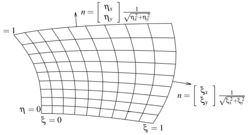
The boundary conditions on the stresses come from a traction boundary condition of the form σn = ¯t where ¯t = (¯tx,¯ty)T is the given traction vector from the fluid and σ is the Cauchy stress tensor in the structure
f g g h
. The unit normaln can be expressed in terms of the coordinate transformation (cf. Figure 1) as n = (1/r)(kx, ky)T and the components of gI and gII for traction boundary conditions can be written as
gI(kx, ky, t) = J−1 r2 1 αr(kx¯tx(k = 1, t) +ky¯ty(k = 1, t)) r¯k ρ˜cs (−ky¯tx(k = 1, t) +kx¯ty(k= 1, t)) , R = 0 −1 1 0 (24) gII(kx, ky, t) = J−1 r2 r¯k ρ˜cs(ky¯tx(k = 0, t)−kxt¯y(k = 0, t)) 1 αr(kx¯tx(k = 0, t) +kyt¯y(k = 0, t)) , L= 0 1 −1 0 (25)
n= ξx ξy 1 √ ξx2+ξy2 n= ηx ηy 1 √ ηx2+ηy2 ξ=0 ξ=1 η=0 η=1
Figure 1: Coordinate transformation
and therefore it is sufficient to specify the two parameters ¯tx and ¯ty on each boundary instead of all of the three ¯f ,¯g,h, which might otherwise violate well-posedness.¯
Inserting the definitions of gI,II and R, L gives with Eq. (17) a SAT expression (which we call simply SAT) for each of the five equations in characteristic variables. For each of the two spatial directions, the transformation matrix T(kx, ky) is applied to get the corresponding SAT expressions in flow variables.
SAT(k)i =T(kx, ky)SAT (k)
i (kx, ky) (26) fork=ξandη. Finally, the total SAT expression is then the sum of the two contributions from the two coordinate directions.
d
SATi,j = SAT (ξ)
i,j(ξx, ξy) + SAT (η)
i,j(ηx, ηy) (27)
5 FLUID-STRUCTURE INTERACTION
5.1 Arbitrary Lagrangean–Eulerian (ALE) formulation
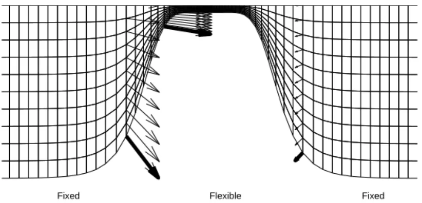
The displacement of the structure interface determines the shape of the fluid domain and the structure velocity at the interface determines the internal grid point velocities in the fluid domain. The right and left boundaries of the fluid domain are the out- and inflow, respectively. The top and bottom parts of the fluid domain are bounded by the flexible vocal folds and the inner wall of the airpipe which is assumed to be rigid. As we do not assume symmetry, the motions of the two vocal folds are solved for individually. In our arbitrary Lagrangean–Eulerian (ALE) formulation, the positions and velocities of the grid points in the fluid domain are linearly interpolated from the positions and velocities of the structures at the interfaces. Figure 2 shows the given structure velocities with bold arrows and the interpolated grid point velocities ˙x,y˙ (thin arrows) for three grid lines.
To obtain the time derivative ofJ−1 as needed in (2), a geometric invariant [17] is used. This geometric conservation law states that (J−1)
Fixed Flexible Fixed
Figure 2: The boundary of the fluid domain consists of fixed and flexible parts. The velocity at the boundary of the flexible part determines the internal grid point velocity. Only half domain shown.
derivatives of the computational coordinatesξ, η can here be obtained from the grid point velocities ˙x,y˙ asξt=−( ˙xξx+ ˙yξy),ηt=−( ˙xηx+ ˙yηy) which can be seen by differentiating the transformation with respect toτ.
5.2 Description of fluid-structure interaction algorithm
At the start of a simulation, we construct the fixed reference configuration for the structure and set the initial variables to zero (no internal stresses and zero velocity). Zero initial conditions are taken for the perturbation variables U0 in the fluid domain (stagnation conditions). In the first time step, the fluid domain is uniquely determined by the reference boundary of the structure. To go from time level n to n+ 1, we first take one time step for the fluid with imposed pressure boundary conditions at the inflow and adiabatic no-slip conditions on the walls, i.e. u = 0 and ∂T /∂n= 0. After the first fluid time step, the viscous fluid stress on the wall is calculated based on the new fluid velocities and pressures. These fluid stresses σf are passed on to the structure solver via the traction boundary condition. The force per unit area exerted on a surface element with unit normal n is ¯t =σfn, where n is here the inward unit normal in the structure, calculated from the displacement vector field.
The traction computed at time levelnfor the fluid is then used to advance the structure solution to time level n+ 1. The solution for the structure at the new time level gives the velocities and displacements on the boundary, which in turn are used to generate the new fluid mesh and internal grid point velocities. This procedure is repeated for each time step.
6 DISCRETIZATION Notation
The Kronecker product of an n×m matrix C and a k×l matrix D is then×m block matrix C⊗D= c11D · · · c1mD .. . . .. ... cn1D · · · cnmD . (28)
This notation will be useful for writing the discretization in a compact form. 6.1 Linear elastic wave equation
Introduce a vector ˆq= (ˆqijk)T = (ˆq001, ...,qˆ005,qˆ101, ...,qˆ105, ...,qˆN M5)T where the three indices i, j and k represent the ξ-coordinate, η-coordinate and the solution variable, re-spectively. We define difference operators in terms of Kronecker products that operate on one index at a time.
Let Qξ = Qξ ⊗IM ⊗I5 and Qη = IN ⊗Qη ⊗I5 where Qξ and Qη are 1D difference operators in the ξ- and η-directions satisfying the SBP property (13). The identity op-erators IN and IM are unit matrices of size (N + 1)×(N + 1) and (M + 1)×(M + 1), respectively. The computation of the spatial differences of ˆqcan then be seen as operat-ing on ˆqwith one of the Kronecker products, i.e. Qηqˆ operates on the second index and yields a vector of the same size as ˆq representing the first derivative approximation in the η-direction. To express the semi-discrete linear elastic wave equation, we also need to define ˆA=IN⊗IM⊗Aˆand ˆB =IN⊗IM⊗B. Note that these products are never actu-ˆ ally explicitly formed as they are merely theoretical constructs to make the notation more compact. The products correspond well to the actual finite difference implementation, i.e. the first derivatives are calculated by operating on successive lines of values in the computational domain. Using the Kronecker products defined above, the semi-discrete linear elastic wave equation with constant coefficients including the SAT expression can be written as
dˆq
dt =Qξ( ˆAˆq) +Qη( ˆBˆq) +
[
SAT (29)
where SAT[ is the SAT expression in transformed coordinates, defined in Eq. (27). 6.2 Navier–Stokes equations
For the fluid equations, we employ a similar procedure, i.e. we define vectors for the solution variables ˆU0 = ( ˆUijk0 )T = ( ˆU0
001, ...,Uˆ 0 004,Uˆ 0 101, ...,Uˆ 0 104, ...,Uˆ 0
N M4)T, and the two flux vectors ˆF0 and ˆG0 similarly defined, where, again, the three indicesi, j andkrepresent the ξ-coordinate, η-coordinate and the solution variable, respectively. The same derivative operators are used as for the linear elastic equation. The discretized fluid equation can
thus be written dUˆ0 dτ =−Qξ ˆ F0−QηGˆ0 (30) 6.3 Time integration
The systems (29) and (30) of ordinary differential equations can readily be solved by the classical 4th order explicit Runge–Kutta method. For the linear elastic wave equation, calling the right-hand side of (29) f(tn,qˆn) at the time level n, we advance the solution to leveln+ 1 by performing the steps
k1 = f(tn,qˆn) k2 = f tn+ ∆t 2 ,qˆ n +∆t 2 k1 k3 = f tn+ ∆t 2 ,qˆ n +∆t 2 k2 k4 = f(tn+ ∆t,ˆqn+ ∆tk3) ˆ qn+1 = ˆqn+ ∆t 6 (k1+ 2k2+ 2k3 +k4)
and similar expressions for the fluid equations (30). The boundary conditions are updated only after all four stages for the respective field have been completed. That is to say, the structure solution at level n + 1 is obtained using only the fluid stress at time level n. Likewise, the fluid solution at time level n+ 1 is based only on the position and velocity of the structure at time level n.
7 RESULTS
Verification
Our fluid solver has previously been verified and tested for numerical simulation of Aeolian tones [13] and qualitatively tested for simulation of human phonation on fixed grids [8] as well as moving grids in ALE formulation [7].
The solver for the linear elastic equations with SAT term has been tested with a manufactured solution and an academic 2D test case in [10] where we obtained a rate of convergence of 3.5 to 4 in 2-norm.
7.1 Problem parameters
The initial geometry for the vocal folds is here based on the geometry used in [19] for an oscillating glottis with a given time dependence. The initial shape of the vocal tract including the vocal fold is given as
rw(x) =
D0−Dmin
4 tanhs+
D0+Dmin
where rw is the half height of the vocal tract, D0 = 5Dg is the height of the channel, Dg = 4 mm is the average glottis height, Dmin = 1.6 mm is the minimum glottis height, s = b|x|/Dg −bDg/|x|, c = 0.42 and b = 1.4. For −2Dg ≤ x ≤ 2Dg, the function (31) describes the curved parts of the reference configuration for the top and bottom (with a minus sign) vocal folds. The x-coordinates for the in- and outflow boundaries are −4Dg and 10Dg, repectively.
7.2 Vocal fold material parameters
The density in the reference configuraiton is ρ0 = 1043 kg/m3, corresponding to the measured density of vocal fold tissue as reported by [6]. The Poisson ratio was chosen as ν = 0.47 for the tissue, corresponding to a nearly incompressible material with ν = 0.5 being the theoretical incompressible limit. The Lam´e parameters were chosen as µ = 3.5 kPa and λ given by λ= 2µν/(1−2ν).
7.3 Fluid model
We used a Reynolds number of 3000 based on the average glottis height Dg = 0.004 m and an assumed average velocity in the glottis ofUm = 40 m/s. We used these particular values in order to be able to compare with previously published results by Zhao et al.
[19, 18] and by ourselves [7, 8]. The Prandtl number was set to 1.0, and the Mach number was 0.2, based on the assumed average velocity and the speed of sound. We deliberately used a lower value for the speed of sound, c0 = 200 m/s in order to speed up the computations. The air density was 1.3 kg/m3 and the atmospheric pressure was patm = 101325 Pa. The equation of state was the perfect gas law, and we assumed a Newtonian fluid. At the inlet, we imposed a typical lung pressure during phonation with a small unsymmetric perturbance by setting the acoustic pressure topacoustic=p−patm = (1 + 0.025 sin 2πη)2736 Pa, where η = 0 at the lower vertex and η = 1 at the upper vertex of the inflow boundary. The outlet pressure was set to atmospheric pressure, i.e. p−patm= 0 Pa.
7.4 Numerical simulation
Both fluid and structure used the same set of variables for nondimensionalization and the same time step was used for both fields so that the two solutions are always at the same time level. The structure grid consisted of 81×61 points for each vocal fold, i.e. for the upper and the lower vocal folds, and the fluid domain was 241×61 points. The time step was determined by the stability condition for the fluid, which was satisfied here by requiring CF L ≤ 1. Since the fluid domain changes with time, the CFL condition puts a stricter constraint on the time step when the glottis is nearly closed. The solution was marched in time with given initial and boundary conditions to dimensional timet = 12 ms (total number of time steps 277310).
would be negligible. After that, the solution was recorded at consecutive 2 ms intervals as shown in Figure 3 where the vorticity is depicted in the left column and the corresponding pressure field is on the right.
Initially, a starting jet is formed in the glottis which becomes unstable near the exit and creates the beginnings of vortical structures at time t= 6 ms. Since the boundary condi-tions are not symmetric with respect to the centerline, also the solution is not symmetric. In the following, vortices are shed near the glottis and propagated downstream driven by the pressure gradient. The pressure plots indicate a sharp pressure drop just before the orifice. Downstream, the pressure minima occur in the vortex centers, as expected.
8 CONCLUSIONS
Our 2D model for the vocal folds based on the linear elastic wave equation in first order form and the air flow based on the compressible Navier–Stokes equations in the vocal tract proves to be able to capture the self-sustained pressure-driven oscillations and vortex generation in the glottis. The high order method for the linear elastic wave equation with a SAT formulation for the boundary conditions ensures a time-stable solution. The fluid and structure fields are simultaneously integrated explicitly in time and boundary data is exchanged only at the end of a time step. With this formulation, there is no need to do iterations in order to find the equilibrium displacement for the structure depending on the fluid stresses. For the problem we consider here, the limiting factor on the time step is the CFL condition from the compressible Navier–Stokes equations. Since the fluid grid has many more grid points, the effort of integrating the linear elastic wave equation, to get the structure displacement, is sub-dominant.
9 ACKNOWLEDGEMENTS
The authors thank Bjørn Skallerud, Paul Leinan and Victorien Prot at the Department of Structural Engineering, NTNU for valuable discussions on the structure model and for Abaqus support. The current research has been funded by the Swedish Research Council under the project ”Numerical Simulation of Respiratory Flow”.
REFERENCES
[1] M. H. Carpenter, D. Gottlieb, and S. Abarbanel. Time-stable boundary conditions for finite-difference schemes solving hyperbolic systems: Methodology and application to high-order compact schemes. J. Comp. Phys., 111:220 – 236, 1994.
[2] B. Fornberg. A Practical Guide to Pseudospectral Methods. Cambridge University Press, 1998.
[3] J.B. Grotberg and O.E. Jensen. Biofluid mechanics in flexible tubes. Annu. Rev. Fluid Mech, 36:121 – 147, 2004.
Figure 3: Vorticity and pressure contours at 2 ms intervals. The left column shows vorticity contours, the right column shows pressure contours. The top row shows the solution evaluated at t = 6 ms, the second row is at t = 8 ms and so on up to t = 14 ms (last row). The colorbar in the vorticity column stretches from 0 to 50 000 s−1and the contour levels are spaced 3 750 s−1apart. For the pressure column,
the inflow is atp=p∞+ ∆p, the outflow is at (approximately)p=p∞and the contour levels are spaced 71 Pa apart.
[4] B. Gustafsson. High order difference methods for time-dependent PDE. Springer-Verlag Berlin Heidelberg, 2008.
[5] B. Gustafsson, H.-O. Kreiss, and J. Oliger. Time Dependent Problems and Difference Methods. John Wiley & Sons, New York, 1995.
[6] E.J. Hunter, I.R. Titze, and F. Alipour. A three-dimensional model of vocal fold abduction/adduction. J. Acoust. Soc. Am., 115(4):1747 – 1759, 2004.
[7] M. Larsson. Numerical Simulation of Human Phonation, Master Thesis, Uppsala University, Department of Information Technology, 2007.
[8] M. Larsson and B. M¨uller. Numerical simulation of confined pulsating jets in human phonation. Computers & Fluids, 38:1375 – 1383, 2009.
[9] M. Larsson and B. M¨uller. Numerical simulation of fluid-structure interaction in hu-man phonation. In B. Skallerud and H.I. Andersson, editors,MekIT 09 Fifth national conference on Computational Mechanics, pages 261 – 280, Trondheim, Norway, 2009. Tapir Academic Press.
[10] M. Larsson and B. M¨uller. Strictly stable high order difference method for the linear elastic wave equation. 2010. Submitted to Commun. Comput. Phys.
[11] R.J. LeVeque. Finite volume methods for hyperbolic problems. Cambridge University Press, 2002.
[12] B. M¨uller. Computation of compressible low Mach number flow, Habilitation Thesis, ETH Z¨urich, 1996.
[13] B. M¨uller. High order numerical simulation of aeolian tones. Computers & Fluids, 37(4):450 – 462, 2008.
[14] T.J. Poinsot and S.K. Lele. Boundary conditions for direct simulations of compress-ible viscous flows. J. Comput. Physics, 101:104 – 129, 1992.
[15] J. Sesterhenn, B. M¨uller, and H. Thomann. On the cancellation problem in cal-culating compressible low Mach number flows. J. Comput. Physics, 151:597 – 615, 1999.
[16] B. Strand. Summation by parts for finite difference approximations for d/dx. J. Comput. Physics, 110:47 – 67, 1994.
[17] M.R. Visbal and D.V. Gaitonde. On the use of higher-order finite-difference schemes on curvilinear and deforming meshes. J. Computat. Physics, 181:155 – 185, 2002.
[18] C. Zhang, W. Zhao, S.H. Frankel, and L. Mongeau. Computational aeroacoustics of phonation, Part II. J. Acoust. Soc. Am., 112(5):2147 – 2154, 2002.
[19] W. Zhao, S.H. Frankel, and L. Mongeau. Computational aeroacoustics of phonation, Part I: Computational methods and sound generation mechanisms. J. Acoust. Soc. Am., 112(5):2134 – 2146, 2002.