Simulation Software for Real Time Forecasting as an Operational Support

Abstract Number 002-0543

Simulation Software for Real Time Forecasting as an Operational Support

Stefan Bjorklund1_{, Naresh Yamani}2_{, Tomas Lloyd}3

1. Linköping Institute of Technology, Linköping University, S 583 81 Linköping Sweden Phone +4613281174 email [email protected].

2. H.No: 8-3-35, Nizampeta, Khammam-507 001 Andhra Pradesh India email [email protected] 3. Rationalia AB, Heidenstams gata 5. 58437 Linköping. Phone +4613172015

Simulation Software for Real Time Forecasting as an Operational Support

1. Linköping Institute of Technology, Linköping University, S 583 81 Linköping Sweden Phone +4613281174 email [email protected].

2. H.No: 8-3-35, Nizampeta, Khammam-507 001 Andhra Pradesh India email [email protected] 3. Rationalia AB, Heidenstams gata 5. 58437 Linköping. Phone +4613172015

email [email protected] ABSTRACT

Simulation has become a more interesting tool for many companies in developed/developing countries to use in different types of production system analysis. Additionally, simulation can be used for operations and not only in the planning or designing phases. Recent advances in

simulation software have allowed simulation to expand its usefulness beyond a purely design function into operational use. The objective is to use the simulation software for the operational support used for scheduling, daily resource allocation, and process monitoring at the same time, identifying all the new features which are available in the Flexsim software. In order to

implement a tool, a virtual production model has been designed to conduct the experiments. In a real time environment all the data has to be retrieved from a company database system but in this work the MS Access database was used to retrieve all the necessary order details.

Keywords: Simulation, operational support, Forecasting

INTRODUCTION

Discrete Event Simulation is a tool that can be used to generate the customized information for decision support. Nowadays simulation is a tool mainly used for different types of production system analysis. But recent advantages in technology have allowed simulation to expand its usefulness beyond a purely design function and into operational use. We have

concluded that the need of a simulation tool to implement any kind of manufacturing system to study a real time forecasting is vital.

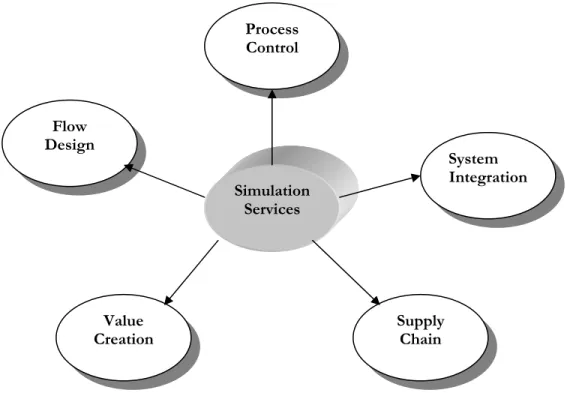
It is difficult to predict software development for even one year; the trends predicted here might be little more than speculation. At present we have many companies providing their own product which can facilitate a more general and also to serve for an individual problems. Most of the products providing with a good graphical user interface and also having options specified by means pull down menus. Many of the tools can accept the other application to connect which gives an add-in feature for example it can able to export or import data from Ms-Excel or other database systems. In manufacturing facility many possible ways to integrate the simulation services between different areas. Today many of the companies integrated with ERP systems, warehouse management systems or at least real time database systems to maintain the material flow. The power of simulation software can be used to connect with the external systems, which further utilized to study the real system. Of course it needs some integration between these systems. This is the basic idea behind this work, how we can implement this methodology in order to solve many shop floor problems to quickly respond to the customers and also to compensate all the uncertainties and disturbances in the system. Another application of such a system, when implementing a model in allocating resources in terms of people, machines and other resources at a terminal. Because the containers come from different places everyday, this will create more problems and complicated if we don’t know how to allocate them properly. Simulating this layout can help to find different storage policies in terms of space and cost of operation. And also it will be easier to find the alternative resource allocation procedures. In other terms the simulation tool is helping us to forecast the model in operational use.

Figure 1: Different Areas to Apply as Operational Support

Nowadays we have more powerful simulations software also available which will need to program either C++ or Visual Basic. And additional programming really performs to solve specialized computations such as scheduling and many other possibilities to customize the model. Flexsim simulation software is a window based application environment. The basic powerfulness comes from its object-oriented technology. It has built by using the current technologies and gives all the power, flexibility and interconnectivity of today’s tools.

The Flexsim is completely integrated with the .NET environment and it also uses flexscript (a C++ precompiled library) and even can write the code in C++. For simulation software the animation is more important to study and show the model to higher levels in the organization, in this software all animation is OpenGL and boasts incredible virtual reality animation. It has the possibility to show all the different views during the model running phase. The virtual reality comes from its 2D, 3D views. It has been used to model manufacturing, warehousing, and material handling processes, semiconductor manufacturing, marine container terminal processes

Simulation Services Process Control Flow Design System Integration Supply Chain Value Creation

and shared access storage network (SANS) simulation. The following section talks about the different areas that we can use this software. The goal of current work is to understand and implement the new features those are available in the Flexsim™ Software. And investigate different methods to design a model to use it for an operational support in a real time environment. The initial condition of the model is the data retrieved from the Company information system usually MPS system.

The main objective of this work will be designed to allocate the target-oriented teams, and also to study the stability of the system by considering few cases.

(a) New orders into the system, which are not in the MPS system. (b) Allocating target oriented teams based on the forecast

(c) Study of model with few operators on leave

(d) Downtime analysis, considering machine failure times.

The number of runs has to be performed for a particular set of data by changing different parameters. Finally the model could be used to analyse the whole system in order to incorporate value addition, financial and costing aspects as well as the expansion of the model to include other parts of the production process.

METHOD

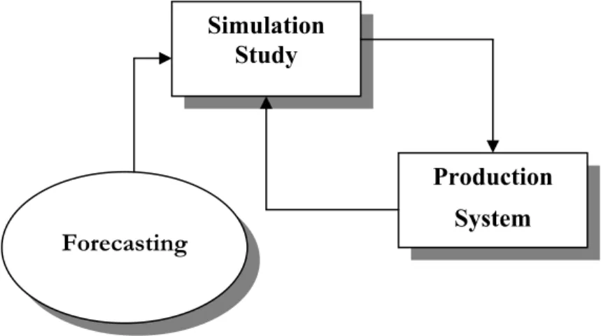
The method is to connect the Simulation model to the company information system (MPS system). If we can define the manufacturing system as a block diagram, in which there are three main modules defined in the diagram, Figure 2.

9 A Simulation study module, in which the whole manufacturing system can be modeled in terms of resources, processes, flow items etc.,

9 A Production system module is the manufacturing facility, where the production work involves.

9 A Forecasting module is the section where it analyzes the updated data from the simulation result as well as historical data to be compared to enhance the production system.

Figure 2: Basic Conceptual Diagram of any Application

The interaction between the Simulation module and the Production System module is an important factor here. The Simulation model has to be updated as per the real system. This can be updated by connecting simulation model with the database of the company information system. Based on the production schedule the time between the simulation runs can be maintained. And it is possible to check any time by running the model at condensed time. The results from the simulation model can be analyzed, but how this forecast information be presented? This could be possible by means of sending the information to the concerned departments before the time. For this there are few possible solutions either sending to the web browser to display the related information (either image or tabular format) or can make it as an understandable form and send it to the different departments.

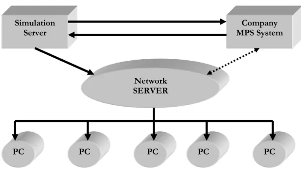
The computer running with simulation is always contacted with the company MPS system to update the information about the material flow. The simulation server can able to send the

Simulation Study

Production System

simulated information to the web server or network server where this server has been connected to the other systems in the production department. Today many companies are doing resource allocation manually by estimating the present situation and deciding where to work and who should work where? The following diagram explains about the detailed method to the information between the servers.

Figure 3: Integrating Different Departments with a Server to send data

It also helps to support in analyzing the scheduling problems. These days we have many scheduling software available from different company providers. It is possible to incorporate that scheduling into the simulation model and see how the behavior of the production system in order to make decisions. The effect on system stability and resource allocation would give an overall cost reduction in a long run of the production. Many other internal disturbances can be studied and make an alert before the production. For example we can even test for an order that is not in the MPS system, whether we can able to deliver before the deadline or not? At another instance

Company MPS System Simulation Server PC PC PC PC PC Network SERVER Various Departments

if few workers will be absent on a particular day within a week, we don’t know how this affects the system stability, these kinds of uncertainties can be included into the Simulation model and tests can be made. It will be a great interest if we can do this experimental analysis in a real time environment in order to implement the real time simulation study. But this could be even possible to build virtual model to analyze different problems and at the same time to finding the affects on the system. But where is the MPS system or company information? From the above diagram it is clear that the simulation model has to interact with the company database, in this case Microsoft Access database has been used to do the experiments. In the following sections the model design and all other assumptions have explained clearly to build the virtual model.

MODEL DESIGN

Basically this model has been built to do the experiments in order to implement the objective of the work. There are many assumptions made in building this model. After building the model the steps in simulation study are applied to it.

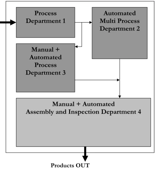
There are four departments in the virtual factory, Figure 4. 1) Process department 1

2) Automated multi process department 2 3) Manual + Automated process department 3

4) Manual + Automated assembly and Inspections department 4

The functional specifications of different departments are given below; this is assumed to make the model.

(1) Process department 1

It is assumed that the material comes from other section in the manufacturing unit. This department consists of 8 machines in which four machines needs an operator for setup and

operational use of the machine. And the other four are automatic machines does require the operator but the negligible time, so not considered while allocating the operators to these machines when the material comes to this section.

Figure 4: Virtual Model Layout Design (2) Automated multi process department 2

It is the second department situated right side from 1st department in the model. This department has got 5 machines, but these machines have the capability to process different operations and of course having a setup time in between. These machines require a dedicated operator but all of these machines are fully automated.

Process

Department 1

Automated

Multi Process

Department 2

Manual + Automated

Assembly and Inspection Department 4

Manual +

Automated

Process

Department 3

(3) Manual and automated process department 3

Actually the products having their unique flow, means based on the product type it has its own way to follow the machines and the departments. This process department consists of 12 machines in which 8 machines require the operator for setup and its operational use.

(4) Manual and automated assembly and inspection department 4

It is the final department, and all of the products must go through this department irrespective of its product type. The products come from department 2 and 3 using a transport. It consists of 20 machines, but all the assembly is not fully automated and needs an operator help on few machines. The inspection is fully automated. The manual assembly utilizes few operators and assuming that the assembly section having enough resource to utilize few more operators if possible to finish the work fast. Based on the products queue the allocation would be made. This is an important department to consider, because if we know the products queue on a particular day before, we could easily make a decision in allocating people to that section. From the above concept the final model has been designed in Flexsim. The full functionality of the model comes from powerful objects provided in Flexsim. In order to build a proper simulation model the input data is necessary. This products arrival data comes from the database connected to the simulation model. And other data required is assumed in the model. The MS access database is used here to implement this model. This data is the real data from the company information system, and it has to be updated before the simulation run. The initial condition of the simulation model is the company current status. All the data from the database is retrieved into the model to run the simulation.

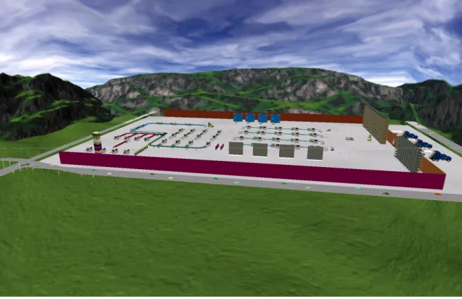
Figure 5 Flexsim designed model

The production schedule is designed and run for 1-week time. And it has three shifts a day (8 hours each shift). While designing the model, it is important to consider the routing of each individual product based on its type. The reason for this is because each product has its own route to follow different machines in each department. In Flexsim the routing could be done either to give an option in send to port of a particular object or can assign all the data in a global table to read it based on the product type. In this model we have used conveyors between different processes and department. This conveyer object gives this functionality.

It is assumed that the production facility can process about 20 different types of products and the routing of each individual product is assigned and given in products flow, Appendix 1.

Model Conceptualization

We have defined few assumptions in the previous topics but in this topic the conceptual model in which all the input factors and level of abstraction will be discussed. And the assumptions in the model have been given at the end of this topic. After building the simulation model, it is important to talk about the different products, which involves in the model.

Product Mix and Product Volume

It is assumed that, there is a lot of different products about 20 different item types involves in the production. Each order may contain different item types and variable quantity. The customer demand can’t be predictable; hence the production facility should capable to resist any product mix with variable volume to deliver the orders in time. This model can also helpful to run the simulation by changing the data like increasing number of orders and at the same time with different product mix and volume.

Level of Abstraction

The level of abstraction is concerned with the level of study required in the model. The following level of details included in the model:

• All products are considered as individual items

• Setup times are included in the objects where required

• Operational times are included in a global table to retrieve data based on the product type

• Operators schedules are stated in a timetables

• The products routing is assigned in the conveyor object

Assumptions

These assumptions are made to run the simulation model efficiently, and the same time to make the model as easy as possible.

• The production schedule is for 1 week to forecast

• The working day has 8 hours per shift and 3 shifts per day and half day on week-ends

• The arrivals into the simulation model is based on the data available in the MS access database (i.e. company information system)

• No rework for product types are necessary

• In the assembly department the enough resources available to work more number of operators.

• The queues in front of the processors have unlimited capacity, it is an important assumption because this data in the assembly section has to be recorded day by day, in allocating the operators.

• The operator’s breakfast and lunch breaks are included, and human factor also considered.

• Transportation times are not included as well as the conveyer times also not included in the model.

• All other relevant data is assumed as and input into the model Data Collection and Database

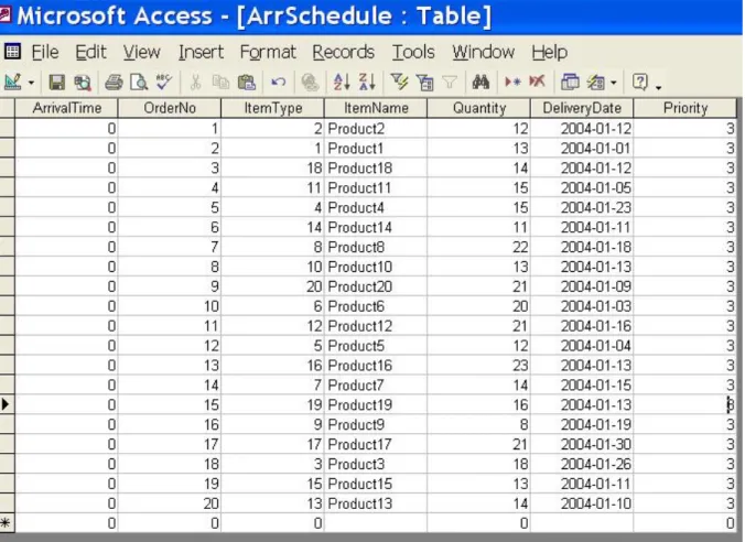
The model has built considering few elements as company information; those are Arrival time, Order Number, Item type, Item Name, Quantity, Delivery date and priority. The last element in the database (i.e. priority) is an additional column, which will help to make few logics to test. Other than this data the following information also needed to input into the model.

• Setup times

• Operational times or Process times

• Shift schedules

• Downtime distributions.

• Products routing Database:

The tables are created in MS access database. In this case the data is entered into the database, each line in the database states that a single arrival of an order. The following table gives an idea about all the elements considered in the database.

SIMULATION EXPERIMENTS

Initially it is assumed that we have 20 orders in the database, when the simulation starts to run all the data from the database is retrieved into the model. With the flexibility of the software, it can be customized to interpret any number of elements as a schedule into the source object. The model has built by using a source object to get the data from the database and it will automatically assign the columns as per the data available in the database.

This model can be tested by increasing the number of orders and can make prioritize based on the requirements. The priority column by default is assigned a number 3; if we assign a lower number can be considered as that product having higher priority. Here it is assumed as the number 1 is a higher priority and 2 are a medium. All objects in the model are fully configured with the capability to take up the higher prioritized product first.

Six individual scenarios were run and the results have analyzed. The input factors of each scenario are almost same as that the orders are retrieved from the Ms Access database and other data for example machine failure rate, absence of operators are inputted based on the scenario type. The database contains about 20 orders with different 20 product types. These orders can have variable quantity and mixture of product types.

The initial conditions are set for each scenario before running the simulation. The experiments which are conducted on the virtual model are as follows:

Scenario 1 General System Analysis and Feasible output

The aim of this scenario is to run the model by scheduling the orders to get a feasible output. Each order having its own delivery date, the simulation can have the ability to prioritize the orders based on its time. It is a very challenging task in any manufacturing concern about which order or arrival have to start first. Normally based on the priority of the order or sometimes the

workers may have their own way to start the work. In both cases the decision may not be correct. But it is possible to run a simulation and make a decision. It is impossible to get an optimal solution by considering all the factors in the production system. But we can get a feasible solution from the model.

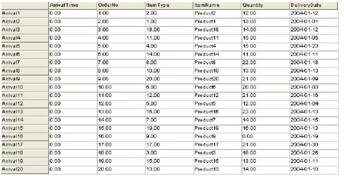
The initial conditions were set, in this case the inputted data in the database, shift schedules etc. The table 2 given below is the data from the database about the arrival schedule. As we have described earlier, it is assumed that the arrival time of the orders which were in the database is zero since these are the current orders to be processed.

Table 2: Retrieved Data in the Source Object

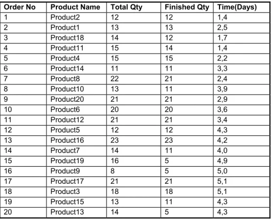
The common shift schedules for the operators are already given before. Now the simulation run was initiated (by pressing Reset button in Flexsim) and run the model for 1 week production time. The total quantity of all the products is 316. After scheduling the orders, the maximum throughput of this model is 290. This resulted data from the simulation model has been exported into an Excel file.

The table 3 shows the maximum output after running the simulation model.

Table 3: General System Resulted Data

It is very clear that this model has few bottleneck problems and also insufficient resources at multiprocessing department. The order numbers 1,2,5,6,9,10,11,12,13,17,18 have finished successfully except the remaining orders. The model also has been analysed by changing the order, in that case we have got very less production output. And there is a considerable work in process in the production by following this product flow into the system.

The state graph shows about the machine idle state to utilization state in percentage, it is an over all percentage in the production period. In the manual assembly section all the machines are waiting for the operators, hence a dedicated operators are important for this section. In the model

Order No Product Name Total Qty Finished Qty Time(Days)

1 Product2 12 12 1,4 2 Product1 13 13 2,5 3 Product18 14 12 1,7 4 Product11 15 14 1,4 5 Product4 15 15 2,2 6 Product14 11 11 3,3 7 Product8 22 21 2,4 8 Product10 13 11 3,9 9 Product20 21 21 2,9 10 Product6 20 20 3,6 11 Product12 21 21 3,4 12 Product5 12 12 4,3 13 Product16 23 23 4,2 14 Product7 14 11 4,0 15 Product19 16 5 4,9 16 Product9 8 5 5,0 17 Product17 21 21 5,1 18 Product3 18 18 5,1 19 Product15 13 11 4,3 20 Product13 14 5 4,3

the operators are allocated between two departments to study the number of operators required. in the scenario 4 discusses about the allocation of operators.

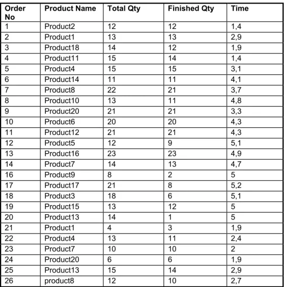
Scenario 2 New Orders into the System which are not in MPS

In this scenario, the input parameters like the operators shifts, the number of orders were kept same as it was in the last scenario. An additional study in this case is, if we receive an immediate order which is not in the database (MPS system), to test whether we can process this order before the delivery time or not. In order to implement this situation an additional orders have taken from the database, while the simulation is running. That means extra orders are inputted into the model at a different arrival time.

The following table shown below, table 4, are the extra orders. And these extra orders entering into the system after a day (i.e. first shift of the second day)

Table 4: Extra Orders - Scenario 2

The resulted output from the simulation is given in table 5, the eight extra orders have inputted but only 6 orders have finished at an adequate quantity. Here we have to notice that the orders number 27, 28 are less prioritized than the other orders; hence those orders have not been processed out. So we were able to deliver the extra orders within the time.

Order

No Product Name Total Qty Finished Qty Time

1 Product2 12 12 1,4 2 Product1 13 13 2,9 3 Product18 14 12 1,9 4 Product11 15 14 1,4 5 Product4 15 15 3,1 6 Product14 11 11 4,1 7 Product8 22 21 3,7 8 Product10 13 11 4,8 9 Product20 21 21 3,3 10 Product6 20 20 4,3 11 Product12 21 21 4,3 12 Product5 12 9 5,1 13 Product16 23 23 4,9 14 Product7 14 13 4,7 16 Product9 8 2 5 17 Product17 21 8 5,2 18 Product3 18 6 5,1 19 Product15 13 12 5 20 Product13 14 1 5 21 Product1 4 3 1,9 22 Product4 13 11 2,4 23 Product7 10 10 2 24 Product20 6 6 1,9 25 Product13 15 14 2,9 26 product8 12 10 2,7

Table 5: Resulted Output - Scenario 2

The total numbers of products are 389 including the new order, and after the production run we were able to finish the products about 299. The above table can be figured out the finished products out of the total quantity. The percentage of work in process is more or less similar to the last scenario. In this case, it can be observed that the processors A1, D1 in the assembly department have blocked with the products about 6-9%, this is because the conveyors in between the processors have the limited capacity, and only one operator working at one processor to assemble. It can be avoided by providing queues before the processor in the assembly section. But the products are expected to assemble continuously to avoid queues in this department.

Scenario 3 Allocating Target oriented Teams Based on the Forecast

This scenario is meant to focus upon the target oriented teams; means in the assembly department 40 % of the machines needs an operator, and it is also possible to allocate more number of operators in order to finish the work fast and also to avoid the products block before this section. We are running the production length for 1 week; from this the forecasted result before the assembly section can be verified. This data has to be sent to the assembly department to alert the operators and it will be useful in allocating them.

The simulation run was performed with the same data used in scenario one, but here we have recorded the queue length in front of the four assembly lines available in the department.

The four queues in front of the 4 assembly lines show the forecast of the queue’s for the coming 7 days, figure 7. Forecast-Queue Content 0 5 10 15 20 25 30 35 40 1 2 3 4 5 6 7

Production Length (Days)

Co n te n t Content at A1 Content at A2 Content at A3 Content at A4

Figure 7 forecast of the queue’s for the coming 7 days

These graphs will show the trends which will enable the production facility to compensate for lack of capacity.

Forecast-Queue Content 0 5 10 15 20 25 30 35 40

Queue A1 Queue A2 Queue A3 Queue A4

Queue Name C ont en t Day 1 Day 2 Day 3 Day 4 Day 5 Day 6 Day 7

Figure 8 Forecast for queue 1-4 for day 1-7

And this information can be utilized by the operators to make a decision about where to work. Now we are using the simulation application as a real time planning tool.

Scenario 4 Increased Number of Orders

In this scenario, the number of orders was increased from 20 to 30 to study the model about its stability and also to find the bottleneck situation at any place arises in the production facility. All other input parameters kept same as in the scenario 1

The total number of 423 products were processed and after the simulation run the resulted output from the excel sheet, Table 7

The output from this scenario is about 300 products. The percentage of work in process is increased by 20% from the first scenario, but we have only increased the products quantity by 35%. And there is no adequate difference in production rate. This is because that we have bottleneck problems in department 2 (Multi processing machines). We can observe that the orders 21, 23 and 26 are only processed, with product types 1, 7, 8 respectively. And these products pass through the departments 1-3-4 and have finished within the production period.

Order No Product Name Total Qty Finished Qty Time(Days)

1 Product2 12 12 1,4 2 Product1 13 13 2,5 3 Product18 14 12 1,7 4 Product11 15 14 1,4 5 Product4 15 15 2,2 6 Product14 11 11 3,3 7 Product8 22 21 2,4 8 Product10 13 11 3,9 9 Product20 21 21 2,9 10 Product6 20 20 3,6 11 Product12 21 21 3,4 12 Product5 12 12 4,3 13 Product16 23 23 4,2 14 Product7 14 11 4 15 Product19 16 5 4,9 16 Product9 8 5 5 17 Product17 21 21 5,1 18 Product3 18 18 5,1 19 Product15 13 11 4,3 20 Product13 14 5 4,3 21 Product1 4 4 4,6 23 Product7 10 8 4,9 26 product8 12 6 5,1

Table 7: Resulted Output - Scenario 4

Because of the constraints like production period and the bottleneck situation at multi processing machines we were unable to finish the other orders. And there is no means available to work

over time and add operators. The only solution is to invest on few more machines or to give buffer period to deliver the orders and finish them in the next week.

Scenario 5 Study of model with Few Operators on Leave

In real time, there are several occasions where the operators may take leave for few days. In this scenario talks about the forecasted result how this phenomenon affects the production, since there are about 12 machines needs an operator for its operational use. The initial condition of the model was set as defined in the 1st scenario except the inputting data about the operator’s absence. The following table shown the time table editor in Flexsim used it to set the 4 operators absence on 3rd day in the week. The four operators took the leave for one day.

The operator’s absence has not very much affected on the production rate, and has got the same figure as in scenario 1. Because it may be the reason on day 3 in the week will not need more operators to work in production. But in real time if we consider more number of products with different product mix may leads to have problems. The absence of operators on different days may also affect the production rate and lead time of the orders. The simulation tool can be used to find the affect of influence of the operator’s absence from day to day to make a decision if they are allowed to take a leave or can find additional workers to replace them.

Scenario 6 Downtime Analysis, Considering Machine failure times

This scenario is only made to know how the machine failure times can affect the production rate. The initial condition was set as per the scenario 1 except the machine break time is introduced. In the production system, it is assumed that there are few machines which have the possibilities to failure. And the time between failures were assumed as an exponential distribution with a location value of 0 and scale value of 1000 using a random number stream 1 i.e. Exponential (0, 1000, 1). All the manually operated machines have configured with this value, which has been set in Flexsim at global MTBF MTTR editor. By introducing the machine failure time, the production output has decreased a little about 2%. We will get a considerable effect if we run the model for long production with a more volume of products, since the product volume is not sufficient for this period of study. Of course it is possible to see much difference by inputting different failure rate, but it is not reasonable to have more failure rates nowadays. With the current technology the failure and break down rates have almost minimized except other factors which are effecting from outside within the factory.

DISCUSSION AND CONCLUSION

The goal of this project work is to develop a methodology to integrate simulation software as a tool to use in a real time operational support. In the overall work we have developed a virtual model to integrate with a database, so that different scenarios have been studied on that model to achieve the objective of the work. This virtual model has been built using an object oriented software “Flexsim” and applied a theory of simulation to perform a successful simulation study. The knowledge about to build a simulation model using “Flexsim” has been analysed carefully to create any kind of real time system to perform similar applications.

It is more important that how we have achieved the objective of the simulation project. Actually it will be very interesting when we implement this model to study in a real time instead of working locally, but this work will be the pathway towards working in real time. Flexsim can synchronise the run with real-time and it has the ability to connect to external systems, warehouse management systems, and ERP systems etc. The real time information can be fed to a Flexsim model and used to monitor and even control of a system in real time. We can see it from the scenarios the forecasted data can be used in allocating the target oriented teams to decide them where to work, as well as in the real time it can be found the forecast error with the resulted data from the simulation run and adjustments could be made. In scheduling the work, the decisions can be easily taken in day by day production as well as it can support to give the production rate and its affect if few operators are absent. In order to compensate the internal disturbances as well the uncertainty in demand, it is always advisable to use simulation software in operational use for decision support. Nowadays there are very few companies using the simulation as real time operational use. The overall project can successfully implement in any kind of manufacturing system, but few things we should keep in mind. The current information

technology is giving an unlimited support to build any kind of system but we have to be thorough with that software (Ex. Flexsim) in order to program as well as to design and customize the model. The analytical and logical thinking are more important for any simulation model specialist.

The integration of the simulation environment in a manufacturing company involves working with the managerial team down to plant floor operators. There is a need to aware the operators to know how we can achieve the improvements by following the real time data from the simulation. In current manufacturing era, it is a biggest challenge to fill the gap between the enterprise systems and the plant shop floor.

All ERP systems which are available for example products from Oracle, PeopleSoft, Microsoft, BaaN, SAP etc would not provide directly a great solution about the forecasting of a real time analysis of any production facility. It would be only possible by integrating simulation software which has the facility to connect the external systems.

The applications of Information Technology has become a key competitive tool in managing the business processes, both within and outside the enterprise, redefining the manufacturing systems effectively and supplier and customer-led business processes. Simulations can drive now in the industry, entrenched in the logistics and supply chain pipeline, with focus on just-in time inventories, shorter production turn around time that can cut down distribution and procurement costs.

If we consider the prospects in manufacturing firms, now we have already had many integrated solutions which include Database systems, ERP, MES and manufacturing Intelligence systems. Now it would be a great interest by integration with real time simulations which I am planning to involve in my feature work. The centralization can be achieved in terms of better support, better

overall visualization, and very simpler interfaces to enterprise systems which lead to E-manufacturing environment.

Flexsim is designed to support a seamlessly integrate simulation software in any manufacturing company or business.

Todays's manufacturing leaders are not only looking all the times the processes to be optimized, but in many cases it is needed to consider all other factors before we make a decision. And we have many third party providers supplying solutions from scheduling tools to optimization tools, but here simulation tools also very predominant to test and find the forecasted results by connecting those tools with the simulation software in order to visualize the whole process to make a decision.

We have an advantage that Flexsim uses Microsoft's C++ compiler, so in addition it is possible to support all the latest distributed technologies providing by the Microsoft.

The other areas to consider building such a real time forecasting could be the use of simulation software for the whole supply chain of the company. This is another challenging task towards the development of infrastructure management.

REFERENCES

Simulation: technologies in the new millennium Davis, W.J.;Simulation Conference Proceedings,

1999. Winter , Volume: 1 , 5-8 Dec. 1999 Pages:141 - 147 vol.1

Using input process indicators for dynamic decision making, Freimer, M.; Schruben, L.;

Simulation Conference Proceedings, 1999. Winter , Volume: 1 , 5-8 Dec. 1999 Pages:325 - 329 vol.1

Using simulation to evaluate buffer adjustment methods in order promising Grant, H.; Moses, S.;

Goldsmann, D.;Simulation Conference, 2002. Proceedings of the Winter , Volume: 2 , 8-11 Dec. 2002 Pages:1838 - 1845 vol.2

Simulation in Manufacturing. Norman Thomson. Research Studies Press LTD, Taunton,

Somerset, England, 1995.

Simulation with Arena, David Kelton, Randdall P. Sadowski and Deborah Sadowski.. McGraw

Hill, New York. 2nd Edition, 2002.

Long-Range Forecasting, From Crystal Ball to Computer. A Wiley-Interscience Publications, J.

Scott, Armstrong. John Wiley & Sons, New York, 1978.

A methodology for improving on-time delivery and load leveling starts Liu, C.; Thongmee, S.;

Hepburn, P.; Advanced Semiconductor Manufacturing Conference and Workshop, 1995. ASMC 95 Proceedings. IEEE/SEMI 1995 , 13-15 Nov. 1995 Pages:95 - 100

Optimal Flow Control in Manufacturing Systems (Production Planning and Scheduling), Oded

Miamon, Eugene Khmelnitsky and Konstantin Kogan. Kluwer Academic Publishers, London, 1998.

Successful Simulation: A Practical Approach to Simulation Projects. Stewart Robinsson.

Manufacturing Planning and Control Systems. Vollmann T.E, Berry, W.L.Whybark. McGraw Hill, New York, 1997.

The merger of discrete event simulation with activity based costing for cost estimation in

manufacturing environments, von Beck, U.; Nowak, J.W.;Simulation Conference

Proceedings, 2000. Winter , Volume: 2 , 10-13 Dec. 2000 Pages:2048 - 2054 vol.2

Tips for Successful Practice of Simulation, D. Sadowski and M. Grabau. Proceedings of the 1999

Winter Simulation Conference.

Proceedings of the 1997 Winter Simulation Conference, .S. Andradottir, K.J. Healy,

D.H.Withers, and B.L.Nelson.

A case study: Simulation and Forecasting in Inter model Container Terminal. Luca Maria

Gambardella, Gianluca Bontempi, Eric Taillard.

Simulation and Real-Time Control. Thompson. M. APICS-The Performance Advantage 8:43-46,

1993.

Proceedings of the 2002 Winter Simulation Conference, E.Yucesan, C.H. Chen, J.L. Snowdon,

and J.M. Chrnes.

Appendix 1 P4 P3 P2 P1 P8 P7 P6 P5 MP1 MP2 MP 3 MP 4 MP 5 D1 P P P P C1 P P P P B1 P P P P A1 P P P P P21 P22 P23 P31 P32 P33 P41 P42 P43 Q Q A4 A3 A2 A1 P51 P52 P53 Types 9-20 Product Types 16-20 11-15 6-10 1-5 Types 1 &2 Types 3& 4 Types 5& 6 Types 7& 8

Products Routing Flow Chart