Copyright by Sungyun Kim 2002

(1)

Copyright by Sungyun Kim

(2)

The Dissertation Committee for Sungyun Kim

certifies that this is the approved version of the following dissertation:

Star-unitary transformation and stochasticity:

emergence of white,

1/f

noise through resonances

Committee:

Ilya Prigogine, Supervisor Tomio Petrosky, Supervisor Mark Raizen

Linda Reichl William Schieve Robert Wyatt

(3)

Star-unitary transformation and stochasticity:

emergence of white,

1/f

noise through resonances

by

Sungyun Kim, B.S.

DISSERTATION

Presented to the Faculty of the Graduate School of The University of Texas at Austin

in Partial Fulfillment of the Requirements

for the Degree of

DOCTOR OF PHILOSOPHY

THE UNIVERSITY OF TEXAS AT AUSTIN December 2002

(4)

(5)

Acknowledgments

It is my pleasure to express gratitude for many people who helped me. I thank Prof. Prigogine for his generosity and showing his unique vi-sion. He showed by example how a person can do scientific research with philosophical vision. I thank Dr. T Petrosky for training me as a physicist. He gave good advices for many of my mistakes and errors. I am very grateful for his patience since I stumbled a lot. I thank Dr. G. Ordonez for encourag-ing me and helpencourag-ing my research. He knows how to make other person’s ideas bloom. His brilliance and honesty really helped me.

I thank Dr. L. Reichl for her kindness when I first came to this center. I thank Dr. W. Schieve, Dr. M. Raizen, Dr. R. Wyatt for generously agreeing to be in my committee. I also thank to Dr. C. Dewitt for her generosity.

Lots of people in Statistical Mechanics center made life here more inter-esting. I thank Annie Harding for her excellent secretary work and helping all the details of center life. I thank Dr. Gursoy Akguc for interesting discussion and comment about physics problems, Anil Shaji for many wonderful informa-tion about India, such as monsoon and elephants. I thank Michael Snyder for showing me nice flashwork, Dario Martinez for the nice wedding party. I thank Chu-Ong ting for his morning greetings and cheerful attitude, Buang Ahn Tay for telling me Buddhist way of life. I am grateful for Dr. Suresh Subbiah for

(6)

his nice personality and good thesis work. I thank Dr. Dean Driebe for teach-ing me many aspects of mappteach-ing, and good advices. I thank Dan Robb for helping dissertation format and many interesting stories. I thank Junghoon Lee for his clarifying ability about math and for being a workout companion, and Jinwook Jung for his cheesecake and discussions about quantum comput-ing. I thank Chun biu Li for many greetings, David Johnson for showing me Tae Kwon do moves, Eshel Faraggi and Wenjun Li for their concern to make the office comfortable.

Of course there are also many people outside the center to whom I am grateful. I thank Jinho Lee for making my laptop more friendly, and his numerous help about other things. Thanks to Keeseong Park, MeeJung Park (for her nice food),

Bonggu Shim, Yunpil Shim, Joonho Bae, Jonghyuk

Kim, Daejin Eom (special thanks), Jihoon Kim, Hoki Yeo, Sungjoon Moon, Donghoon Chae, Soyeon Park, Yongjung Lee, Wanyoung Jang, Suhan Lee, Hongki Min (for easing the tension), Sangwoo Kim, Sungwhan Jung, Ky-oungjin Ahn, Yunsik Lee, Deayoung Lim, Mrs Prigogine, Ricardo, Marcello, Stephanie, Dr. Karpov.

(7)

Star-unitary transformation and stochasticity:

emergence of white,

1/f

noise through resonances

Publication No.

Sungyun Kim, Ph.D.

The University of Texas at Austin, 2002 Supervisors: Ilya Prigogine

Tomio Petrosky

In this thesis we consider the problem of stochasticity in Hamiltonian dynamics. It was shown by Poincar´e that nonintegrable systems do not have constants of motion due to resonances. Divergences due to resonances ap-pear when we try to solve the Hamiltonian by perturbation. In recent years, Prigogine’s group showed that there may exist a new way of solving the Hamil-tonian by introducing a non-unitary transformation Λ which removes the di-vergences systematically. In this thesis we apply this Λ transformation to the problem of stochasticity.

To this end, first we study classical Friedrichs model, which describes the interaction between a particle and field. For this model we derive the Λ transformation for general functions of particle modes, and show that the Langevin and Fokker-Planck equations can be derived through the transformed particle density function. It is also shown that the Gaussian white noise struc-ture can be derived through the removal of divergences due to resonances. We

(8)

extend this to the quantum case, and show that the same structure can be preserved if we keep the normal order of creation and destruction operators. We also study the extended Friedrichs model. This model can be mapped from the case in which a small system is weakly interacting with a reservoir. In this model we show that low frequency 1/f noise is derived due to the sum of resonances effect.

(9)

List of Figures

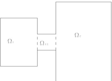
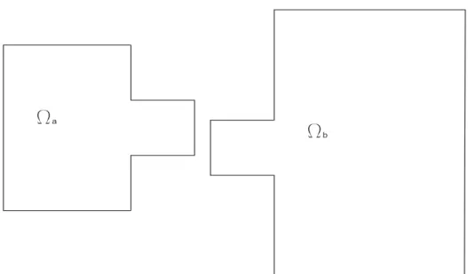
6.1 The system . . . 68 6.2 Ωa and Ωb . . . 70

(13)

Chapter 1 Introduction

The contents of chapter 1 - chapter 4 are based on the papers [1] [2], in which the author and G. Ordonez closely collaborated. Author deeply appreci-ated that.

In this thesis we study the connection between Hamiltonian dynamics and irreversible, stochastic behavior, like decay, Brownian motion and noises. In classical physics the basic laws are time reversible. If we know the Hamiltonian, then we get Hamilton’s equations of motion which describe the time evolution of the system in a time reversible, deterministic way. On the other hand, we see time irreversibility and stochastic behavior everywhere. How to bridge the gap between theory and this reality is one of main theme of this thesis. We explicitly show that how resonance is related to the irre-versibility and stochasticity.

A simple stochastic irreversible equation is the Langevin equation, de-scribing Brownian motion of a particle. For example, we can write a Langevin equation for a particle with mass m under the harmonic potential mω2_x2_/_2,

(14)

term γdx(t)/dt with constant γ and a white noise term ξ(t) to the harmonic oscillator equation, we get

m d 2 dt2x(t) +mγ d dtx(t) +mω 2_x₍_t_{) =}_ξ₍_t₎_. _(1.1)

The damping and noise terms represent the effect of the environment of the particle. To study the same system dynamically, we construct a Hamiltonian which serves as a model of the particle and its environment [3]. This can be done both in classical and quantum mechanics. As shown by Mori and others (see [4] and references therein), starting with the Hamiltonian (or Heisenberg) equations of motion, one can derive generalized Langevin-type equations. For example, for the particle in the harmonic potential one can model the envi-ronment as a set of harmonic oscillators (bath) linearly coupled to the particle (the Caldeira-Legget model [3]). This gives the exact equation [5, 6]

md 2 dt2x(t) + Z t 0 dt0γb(t−t0) dx(t0) dt0 +mω 2_x₍_t₎ =ξb(t)−x(0)γb(t), (1.2)

whereγb(t) andξb(t) are functions of the bath degrees of freedom and their cou-pling to the particle. This equation is equivalent to the original Hamiltonian equations, and therefore it is both time-reversal invariant and deterministic1_.

In contrast, the Langevin equation (1.1) has broken-time symmetry and contains a random force. The question is how to relate this phenomenological equation to Hamiltonian dynamics, represented by Eq. (1.2). A main difference

(15)

between Eqs. (1.1) and (1.2) is that the first is “Markovian,” for thex and p, and it has no memory terms, while the second is “non-Markovian:” it has a memory term that makes the value of x(t) dependent on the velocities at all the previous times t0.

A standard argument to derive Eq. (1.1) from Eq. (1.2) is to focus on time scales of the order of the relaxation time for the weak coupling case. Then the functionγb(t) can be approximated by the delta functionγδ(t−0±) [6]. In this procedure time-symmetry is broken as one has to choose between the delta functions δ(t−0±) for t > 0 or t < 0, respectively. Further approximations like averging out rapidly oscillating terms [8] show that the termξb(t) can be replaced by the white noise term ξ(t). Then for t > 0 we obtain Eq. (1.1) from Eq. (1.2) with γ > 0 [for t < 0 we change γ ⇒ −γ]. All this amounts to a “Markovian” approximation, where the memory terms in both γb and the noise correlation are dropped. This corresponds to theλ2_t _{approximation}

[9–12].

So, is Eq. (1.1) the result of an approximation? If this is so, this im-plies that both irreversibility and stochasticity are results of approximations. In chapter 4 we point out that irreversible and stochastic equations such as (1.1) can be viewed in a different way: they describe the time evolution of components of dynamics. This view has been put forward by Prigogine and collaborators [14]-[24]. We will show that indeed there are components ex-actly obeying Langevin (or Fokker-Planck) time evolution. These components are obtained by isolating resonant contribution. Thus we can also say that

(16)

resonance gives Gaussian white noise. We will consider the Friedrichs model, and we will consider classical mechanics. Later, for the 1/f type noise, we consider extended Friedrichs model. In this model we also show that the sum of resonance contributions gives the 1/f noise.

The outline of deriving the irreversible and stochastic components is the following. The system is described by a Hamiltonian

H =H0+λV (1.3)

where H0 describes the unperturbed system without any couplings, V

de-scribes the interactions and λ is the dimensionless coupling constant. The associated Liouville operator or Liouvillian, i.e., the Poisson bracket with the Hamiltonian, is LH = i{H, }. This is also written as LH = L0+λLV. The time evolution of any function of the phase space variables f(x, p) is given by

df

dt =iLHf (1.4)

We distinguish between integrable and nonintegrable systems.

For integrable systems one can introduce a canonical “unitary” trans-formation U that simplifies enormously the equations of motion. The trans-formationU−1 _{is applied to phase-space variables. The new variables describe}

non-interacting particles (quasiparticles). In the new representation we have periodic motion and there are no irreversible, stochastic processes. We obtain trivial Markovian equations with zero damping and no noise [see Eq. (3.33)]. After solving the trivial equations, we can transform the solutions back to the original phase-space variables.

(17)

But integrable systems are exceptional. Most systems are noninte-grable, at least in the sense of Poincar´e. This means thatU is not an analytic function of the coupling constant atλ= 0, and hence it cannot be constructed by perturbation expansions. This is due to resonances that produce vanishing denominators leading to divergences.

Prigogine and collaborators have introduced a “star-unitary” mation Λ, that has essentially the same structure as the canonical transfor-mation U, but with regularized denominators. As we will discuss later, star-unitarity is an extension of star-unitarity from integrable to nonintegrable systems. The regularization in Λ eliminates the divergences due to resonances. At the same time, it brings us to a new description that is no more equivalent to free motion. We have instead a “kinetic” description in terms of quasiparti-cles that obey simpler Markovian equations, but still interact. After solving these equations we can (at least in principle) go back to the original variables to solve the original equations of motion. The main point is that Markovian irreversible equations such as (1.1) describe components of the motion of the particles. In this thesis we will focus on the components leading to Brownian motion.

How is it possible that Hamiltonian dynamics can yield irreversible equations? This is because the Λ-transformed phase-space functions involve generalized functions, or distributions (examples are the “Gamow modes” pre-sented in Sec. 3.3). If the initial unperturbed functions formed a Hilbert space, the transformed functions are no more in this Hilbert space. In its transformed

(18)

domainLH behaves as a dissipative collision operator with complex eigenval-ues [19, 20]. The extension of LH involves an extension of real frequencies to complex frequencies, which breaks time-symmetry. We remark that even though the Hamiltonian H is time reversal invariant, breaking of time sym-metry can occur in thesolutionsof the equations of motion. For example, the harmonic oscillator coupled to the bath can be exponentially damped either towards the future or the past. The two types of solution are possible. This is closely connected to the existence of eigenfunctions ofLH that break time-symmetry. We also note that damping and other irreversible processes occur only for systems that can have resonances, and are nonintegrable in the sense of Poincar´e.

In order to construct Λ we specify the following requirements:

(1) The Λ transformation is obtained by analytic continuation of the unitary operatorU.

(2) When there are no resonances, Λ reduces toU.

(3) Λ is analytic with respect to the coupling constant λ at λ= 0. (4) Λ preserves the measure of the phase space.

(5) Λ maps real variables to real variables.

(6) Λ leads to closed Markovian kinetic equations.

In addition, to obtain a specific form of Λ we consider the “simplest” extension of U. This will be seen more precisely later, when we study our specific Hamiltonian model [see Eq. (A.24) and comments below].

(19)

In quantum mechanics, the Λ transformation has been used to define a dressed unstable particle state that has strict exponential decay. This state has a real average energy and gives an uncertainty relation between the lifetime and energy [17, 22, 25]. The dressed state defined by Λ has an exact Markovian time evolution, without the Zeno [26] or long tail periods [27].

The Friedrichs model we will consider describes a charged particle in a harmonic potential, coupled to a field bath. We are interested in the infinite volume limit of the systemL→ ∞. The emission of the field from the particle leads to radiation damping. Conversely, the particle is excited when it absorbs the field. Depending on the initial state of the field, we have two distinct situations: (a) The field is in a “thermodynamic” state and (b) the field is in a “non-thermodynamic” state. The first case occurs when the the average action hJkiof each field mode k satisfies [28]

hJki ∼O(L0) (1.5)

Then the total energy is proportional to the volume L. This corresponds to the “thermodynamic limit.” It does not necessarily imply that the field is in thermal equilibrium; it just means that we have a finite (non vanishing) energy density in the limit L→ ∞. The existence of the thermodynamic limit requires an initially random distribution of the phases of the field modes [29]. The second (“non-thermodynamic”) case occurs when we havehJki ∼O(L−1), i.e., we have a vanishing energy density.

(20)

damped oscillation, the particle undergoes an erratic motion due to the ex-citation caused by the thermodynamic field. This erratic motion includes a Brownian motion component, which is Markovian. The initial randomness of the phases of the field modes is a necessary condition for the appearance of Brownian motion. In addition it is essential that the field resonates with the particle. We need Poincar´e resonances. Under these conditions Λ permits us to isolate the damping and the Brownian component of the motion. In phenomenological theories Brownian motion is attributed to a Gaussian white noise source, which creates fluctuations. In our formulation the effects of fluc-tuations are originated in the nondistributive property of Λ with respect to multiplication of dynamical variables. Nondistribuitivity is a consequence of the removal of Poincar´e divergences. Later for the extended Friedrichs model, we show that the sum of resonance effects gives 1/f noise effect.

The organization of this thesis is as follows. In chapter 2 we introduce Λ transformation as an extended version of unitary transformation in the non-integrable systems. In chapter 3 we introduce the Friedrichs Hamiltonian and find Λ transformation. In chapter 4 we show that this transformation leads to Langevin and Fokker-Planck equations, and classical Gaussian white noise. In chapter 5 we briefly discuss the properties of quantum noise. In chapter 6 we introduce an extended Friedrichs model for the electron waveguide cavity, and derive the 1/f noise as sum of resonance contributions. In conclusion we summarize our results.

(21)

Chapter 2 Non-integrable systems and star-unitary

transformation

2.1 Integrable and non-Integrable systems

We study a system of particles with Hamiltonian

H =H0+λV, H =H(p, q) (2.1)

whereH0is the unperturbed Hamiltonian describing non-interacting particles,

and V is the interaction. We assume the coupling constant λ is dimension-less. We consider mainly classical systems, but our statements apply as well to quantum systems. The Hamiltonian is a function of the momentap and posi-tionsqof the particles. Often one introduces a new set of variablesJ =J(p, q),

α=α(p, q) (action-angle variables) such that

H0 =H0(J), V =V(J, α) (2.2)

This means that when there is no interaction between the particles (λ = 0) the energy H only depends on the action variablesJ.

Integrable systems are systems for which we can go to a new represen-tationJ ⇒J¯, α⇒α¯ such that

(22)

The Hamiltonian can be written as a new function ¯H0 depending only on

the new actions. Typically, ¯H0 will have the same form as H0, but with

renormalized parameters (such as frequencies).

The change of representation is expressed as a “canonical transforma-tion”U,

¯

J =U−1J, α¯=U−1α (2.4)

The operatorUis “unitary,”U−1 ₌_U†_{, where we define Hermitian conjugation}

through the inner product

hhf|ρii= Z

dΓf∗(Γ)ρ(Γ). (2.5) which is the ensemble average off.1 _{Here Γ is the set of all phase space}

vari-ables,dΓ is the phase-space volume element and ∗means complex conjugate. The Hermitian conjugate is defined by

hhf|U ρii=hhρ|U†fii∗ (2.6) The operator U is distributive with respect to products. For any two variablesA and B we have [34]

U AB = (U A)(U B) (2.7)

This property together with Eq. (2.3) lead to

U H(J, α) = UH¯0( ¯J) = ¯H0(UJ¯) = ¯H0(J) (2.8)

1_{One can introduce a Hilbert-space structure in classical mechanics through the}

(23)

The transformed Hamiltonian U H is the unperturbed Hamiltonian ¯H0

de-pending only on the original action variables. In other words, U eliminates interactions.

The solution of the total HamiltonianHcan be found easily through the unitary transformationU. We look for the solution of the Hamiltonian through the Liouville equation which describes the time evolution of the statistical ensemble. For systems with many degrees of freedom the Liouville equation has an advantage since it can summarize the behavior of the whole system in a single equation. The statistical ensemble ρsatisfies the Louville equation

i∂

∂tρ=i{H, ρ}=LHρ (2.9)

whereLH =i{H, } is the Liouville operator or Liouvillian. Similar to H,LH may be split into a free Liouvillian plus interaction: LH = L0 +λLV, where

L0 =LH0. ApplyingU on both sides of the Liouville equation we get

i∂ ∂tU ρ = U LHU −1 U ρ ⇒i∂ ∂tρ¯ = ¯ L0ρ¯ (2.10) where ¯ ρ=U ρ, L¯0 =U LHU−1. (2.11) ¯

L0 has the form of the non-interacting Liouvillian. Indeed We have

¯

L0ρ¯=iU{H, ρ}=i{U H, U ρ}

(24)

where in the second equality we used the property of preservation of the Pois-son bracket by canonical transformations [34]. The transformed Liouvillian

¯

L0 does not contain any interaction terms, and the ensemble average over this

transformed density function ¯ρ can be easily calculated when the solution for ¯

H is known.

For non-integrable systems there exist, by definition, no transformation

U. This happens, for example, when there appear divergences (divisions by zero) when we try to construct U as an expansion in the coupling constant

λ (called “perturbation expansion”). Vanishing denominators appear when frequencies of the systems become equal. We have “Poincar´e resonances” leading to divergences [16],

1

ω1−ωk

→ ∞ forω1 →ωk (2.13)

We define now a transformation Λ with the following properties:

(1) The Λ transformation is obtained by analytic extension of the uni-tary operator U which diagoanlize the Hamiltonian .

(2) When there are no resonances, Λ reduces toU.

(3) Λ is analytic with respect to the coupling constant λ at λ= 0. (4) Λ preserves the measure of the phase space.

(5) Λ maps real variables to real variables.

(25)

Our method corresponds to the elimination of Poincar´e resonances on the level of distributions. This extension ofU is obtained by regularization of the denominators, 1 ω1−ωk ⇒ 1 ω1−ωk±i (2.14) where is an infinitesimal. As discussed below, the sign of i is determined by a time ordering depending on the correlations that appear as the particles interact. The regularization breaks time symmetry.

The Λ transformation permits us to find new units obeying kinetic equa-tions. Indeed, applying the Λ transformation to the equations of motion, we discover irreversibility and stochasticity. Irreversibility appears because of the analytic continuation ofU (from real to complex frequencies) and stochasticity because of the non-distributive property

ΛAB6= (ΛA)(ΛB). (2.15) Hence we have fluctuations. Irreversibility and stochasticity are closely related to Poincar´e resonances [13–15].

We introduce the new distribution function ˜ρ = Λρ into the Liouville equation. Then we obtain

i∂

∂tρ˜= ˜θρ˜ (2.16)

where

˜

(26)

This is a kinetic equation describing irreversible stochastic phenomena. This equation in general contains diffusive terms, which map trajectories to ensem-bles. We have an intrinsically statistical formulation in terms of probabilities. The next section will be devoted to a brief description of the main steps involved in the construction of the Λ transformation (more details can be found in Refs. [22, 25] and references therein for quantum mechanics, and in Ref. [24] for classical mechanics).

2.2 Construction of the

Λ

transformation

Our formulation is based on the “dynamics of correlations” induced by the Liouville equation [7]. The Liouville operatorLH =L0+λLV is separated into a part describing free motion L0 = i{H0, } and an interaction λLV =

i{λV, }. We then define correlation subspaces by decomposing the density operatorρ into independent components

ρ =X ν

P(ν)ρ (2.18)

whereP(ν) are projectors to the orthogonal eigenspaces of L0

L0P(ν) =P(ν)L0 =w(ν)P(ν) (2.19)

w(ν) _{being the real eigenvalues of} _L

0. The projectors are orthogonal and

com-plete:

P(µ)P(ν) =P(µ)δµν,

X ν

(27)

The complement projectorsQ(ν) _{are defined by}

P(ν)+Q(ν) = 1 (2.21)

They are orthogonal toP(ν)_{, i.e.,}_Q(ν)_P(ν)₌_P(ν)_Q(ν) _{= 0, and satisfy [}_Q(ν)_]2 ₌

Q(ν)_.

As seen in Eq. (2.19) the unperturbed Liouvillian L0 commutes with

the projectors. Therefore the unperturbed Liouville equation is decomposed into a set of independent equations,

i∂ ∂tP

(ν)_ρ₌_L

0P(ν)ρ=w(ν)P(ν)ρ (2.22)

The interactionλLV induces transitions from one subspace to another subspace. To each subspaceP(ν) we associate a “degree of correlation”dν: we first define the vacuum of correlation as the set of all distributions belonging to the P(0) _{subspace. This subspace by definition has a degree of correlation}

d0 = 0. Usually this subspace has the eigenvalue w(0) = 0, i.e., it contains the

invariants of unperturbed motion. The degree of correlation dν of a subspace

P(ν) _{is then defined as the minimum number of times we need to apply the}

interaction LV on the vacuum of correlationsP(0)in order to make a transition to P(ν). Dynamics is seen as a dynamics of correlations.

Our method involves the extension of U to Λ, from integrable to non-integrable systems. This is applicable to systems, which, depending on certain parameters, can be either integrable or non-integrable in the sense of Poincar´e. For example, a system contained in a finite box with periodic boundary con-ditions will have a discrete spectrum of frequencies. We can then avoid any

(28)

resonances. The system is integrable, and we can construct U by perturba-tion expansions. However, when we take the limit of an infinite volume, the spectrum of frequencies becomes continuous and resonances are unavoidable. The system becomes non-integrable in Poincar´e’s sense, as the perturbation expansion of U gives divergent terms. We can remove the divergences by regularization of the denominators, obtaining the Λ transformation.

Let us consider first integrable systems, where we may introduce the canonical transformationU that eliminates the interactions. In the Liouvillian formulation the relation (2.8) gives

U LHU−1 = ¯L0 (2.23)

Namely, the transformed Liouvillian is the unperturbed Liouvillian ¯L0 =

i{H¯0, }. Similar to L0 we have

¯

L0P(ν) =P(ν)L¯0 = ¯w(ν)P(ν) (2.24)

where ¯w(ν) are renormalized eigenvalues. In the U representation there are no transitions from one degree of correlation to another.

We write U in terms of “kinetic operators” (we use bars for the inte-grable case)

¯

χ(ν)≡P(ν)U−1P(ν) (2.25) ¯

(29)

We have as well the hermitian conjugate components

[ ¯χ(ν)]†≡P(ν)U P(ν) (2.26) [ ¯χ(ν)]†D¯(ν) ≡P(ν)U Q(ν)

where ¯D(ν) ≡ [ ¯C(ν)]†. The operators ¯C(ν) and ¯D(ν) are called, respectively, “creation” and “destruction” operators [14] as they can create or destroy cor-relations, leading to transitions from one subspaceP(ν) _{to a different subspace}

P(µ)_{. The ¯}_χ(ν) _{operator, on the other hand, is diagonal, as it leads to}

tran-sitions within each subspace, i.e., it maps P(ν) _to _P(ν)_{. Using Eq. (2.21) we}

obtain

U−1P(ν) = (P(ν)+ ¯C(ν)) ¯χ(ν) (2.27)

P(ν)U = [ ¯χ(ν)]†(P(ν)+ ¯D(ν)) (2.28) Now, from the commutation relation in Eq. (2.24) we derive a closed equation for the ¯C(ν) _{operators. From Eq. (2.24), we have}

LHU−1P(ν)=U−1P(ν)U LHU−1P(ν), (2.29) Substituting Eq. (2.27) into Eq. (2.29), we get

LH(P(ν)+ ¯C(ν)) ¯χ(ν) = (P(ν)+ ¯C(ν)) ¯χ(ν)U LH(P(ν)+ ¯C(ν)) ¯χ(ν). (2.30) Let us write

¯

(30)

Multiplying ¯Φ(_Cν) on both sides of Eq. (2.30) by left, we get ¯ Φ(_Cν)LHΦ¯ (ν) C χ¯ (ν)_{= ¯}_Φ(ν) C χ¯ (ν)_{U L} H(P(ν)+ ¯C(ν)) ¯χ(ν) =LHΦ¯ (ν) C χ¯ (ν) _(2.32) where we used ( ¯Φ(_Cν))2 _{= ¯}_Φ(ν)

C and Eq. (2.30) again. The relation ( ¯Φ

(ν)

C )2 = ¯Φ

(ν)

C comes from the fact

(P(ν))2 =P(ν), P(ν)C¯(ν) = 0, (2.33) ( ¯C(ν))2 = 0, C¯(ν)P(ν)= 0. (2.34) So we have ¯ Φ_C(ν)LHΦ¯_C(ν)=LHΦ¯(_Cν) (2.35) (w(ν)−L0) ¯Φ (ν) C =λLVΦ¯ (ν) C −Φ¯ (ν) C λLVΦ¯ (ν) C . (2.36)

From Eq. (2.36) we get a closed equation for ¯Φ(_Cν), ¯ Φ(_Cν)=P(ν)+ X µ(6=ν) P(µ) −1 w(µ)₋_w(ν)[λLVΦ¯ (ν) C −Φ¯ (ν) C λLVΦ¯ (ν) C ] (2.37) or ¯ C(ν) = X µ(6=ν) P(µ) −1 w(µ)₋_w(ν) (2.38) × [λLVP(ν)+λLVC¯(ν)−C¯(ν)λLVC¯(ν)].

We call Eq. (2.37) the nonlinear Lippmann-Schwinger equation. The ¯χ(ν)

operators are obtained from the relation

(31)

which leads to [22]

¯

A(ν)= ¯χ(ν)[ ¯χ(ν)]† (2.40) where ¯A(ν) _≡ ₍_P(ν) _{+ ¯}_D(ν)_C_¯(ν)₎−1 _{(the inverse is defined in each subspace:}

¯

A(ν)_{[ ¯}_A(ν)_]−1 ₌_P(ν)_{). The general solution of Eq. (2.39) is}

¯

χ(ν) = [ ¯A(ν)]1/2exp( ¯B(ν)) (2.41) where ¯B(ν) ₌ _{−[ ¯}_B(ν)_]† _{is an arbitrary antihermitian operator. For the}

in-tegrable case we have one more condition on U: the distributivity property Eq. (2.7). This condition fixes the operator ¯χ(ν) _{(see Appendix A). Note that}

for integrable systems the denominator in Eq. (2.38) is always non-vanishing: there are no Poincar´e resonances.

Now we go to nonintegrable systems. Due to Poincar´e divergence we cannot eliminate the interactions among particles through a canonical trans-formation. However we may still introduce a representation for which the dynamics is closed within each correlation subspace. We introduce the trans-formation Λ such that the transformed Liouvillian in Eq. (2.17) commutes with the projectorsP(ν)

˜

θP(ν) =P(ν)θ˜ (2.42) This allows us to obtain closed Markovian equations

i∂ ∂tP

(ν)

˜

ρ= ˜θP(ν)ρ˜ (2.43)

In contrast to the integrable case, the P(ν) _{projectors are no more}

(32)

each subspace. As we shall show, the Λ transformation makes a direct connec-tion between dynamics and kinetic theory. The operator ˜θ is indeed a gener-alized “collision operator.” Collision operators are familiar in kinetic theory. They are dissipative operators with complex eigenvalues, the imaginary parts of which give, for example, damping or diffusion rates. The Liouville operator is related to ˜θ through a similitude relation. This means that LH itself has complex eigenvalues. This is possible because we are extending the domain of

LH to distributions outside the Hilbert space [18, 20, 22].

To construct Λ, the basic idea is to extend the canonical transformation

U through analytic continuation. Similar to Eq. (2.27) we write Λ in terms of kinetic operators

Λ−1P(ν) = (P(ν)+C(ν))χ(ν) (2.44)

P(ν)Λ = [χ(ν)]?(P(ν)+D(ν))

In order to avoid Poincar´e divergences, Λ can no more be unitary. Instead, it is “star unitary”

Λ−1 = Λ? (2.45)

where the?applied to operators means “star-hermitian” conjugation, defined below.

From the commutation relation Eq. (2.42) we arrive again at the equa-tion (2.38) for the creaequa-tion operator. But the denominator in Eq. (2.38) may now vanish due to Poincar´e resonances. We regularize it by adding ±i. We

(33)

obtain the equation Φ(_Cν) =P(ν)+ X µ(6=ν) P(µ) −1 w(µ)₋_w(ν)₋_i µν [λLVΦ (ν) C −Φ (ν) C λLVΦ (ν) C ] (2.46) or C(ν) = X µ(6=ν) P(µ) −1 w(µ)₋_w(ν)₋_i µν (2.47) × [λLVP(ν)+λLVC(ν)−C(ν)λLVC(ν)]

where the sign if i is chosen according to the “i-rule:” [20, 22]

µν = + if dµ≥dν (2.48)

µν =− if dµ< dν

where > 0. This rule means, essentially, that transitions from lower to higher correlations are oriented towards the future and transitions from higher to lower correlations are oriented towards the past. We could also choose the other branch with <0, where the roles of past and future are exchanged. The main point is that regularization of the denominators breaks time symmetry.

For theD(ν) _{operators we have}

D(ν) = [P(ν)λLV +D(ν)λLV −D(ν)λLVD(ν)] (2.49) × X µ(6=ν) 1 w(ν)₋_w(µ)₋_i νµ P(µ)

The i-rule leads to well defined perturbation expansions for C(ν)_, _D(ν) _and

(34)

for the integrable case. For the non-integrable case, due to i rule, these operators are no more related by hermitian conjugation. They are related by star hermitian conjugation, which is obtained by hermitian conjugation plus the change µν ⇒νµ. Then we have

D(ν) = [C(ν)]?, A(ν)= [A(ν)]? (2.50) Similar to the integrable case the χoperators are given by

χ(ν) = [A(ν)]1/2exp(B(ν)) (2.51) where B(ν) = −[B(ν)]? is an arbitrary anti-star-hermitian operator. In con-trast to the integrable case we have no distributivity condition to deriveB(ν). However, the conditions on Λ stated before lead to a well definedχ(ν)operator.

(35)

Chapter 3 The Friedrichs model and

Λ

transformation

3.1 The classical Friedrichs model

We consider a classical system consisting of a charged harmonic oscil-lator coupled to a classical scalar field in one-dimensional space. A quantum version of this model has been studied by Friedrichs [31], among others. We write the Hamiltonian of the system in terms of the oscillator and field modes ¯ q1 and ¯qk, H = H0+λV (3.1) = ω1q¯1∗q¯1+ X k ωkq¯∗kq¯k+λ X k ¯ Vk(¯q1∗q¯k+ ¯q1q¯∗k),

with a given constant frequency ω1 >0 for the harmonic oscillator (particle),

c= 1 for the speed of light,ωk =|k|for the field, and a dimensionless coupling constant λ 1_{. When} _λ _{is small we can treat the interaction potential as a}

perturbation. We assume the system is in a one-dimensional box of sizeLwith periodic boundary conditions. Then the spectrum of the field is discrete, i.e.,

k = 2πj/L where j is an integer. The volume dependence of the interaction

1_{In Ref. [24], we used a dimensionless Hamiltonian dividing the Hamiltonian by a}

con-stantω0J0. In this Hamiltonian, all variables become dimensionless. This is more convenient

(36)

Vk is given by ¯ Vk = r 2π L ¯vk (3.2)

where ¯vk=O(1). We assume that ¯vk is real and even: ¯vk = ¯v−k. Furthermore, we assume that for small k

¯

vk ∼ω

1/2

k . (3.3)

To deal with the continuous spectrum of the field we take the limit

L→ ∞. In this limit we have 2π L X k → Z dk, L 2πδk,0 →δ(k). (3.4)

The normal coordinates ¯q1, ¯qk satisfy the Poisson bracket relation

i{¯qα, q¯∗β}=δαβ. (3.5) where i{f, g}= X r=1,k h∂f ∂q¯r ∂g ∂q¯∗ r − ∂g ∂q¯r ∂f ∂q¯∗ r i (3.6) The normal coordinates are related to the position x1 and the momentum p1

of the particle as ¯ q1 = r mω1 2 (x1 + ip1 mω1 ), (3.7) x1 = 1 √ 2mω1 (¯q1+ ¯q∗1), p1 = −i r mω1 2 (¯q1−q¯ ∗ 1) (3.8)

(37)

and to the fieldφ(x) and its conjugate fieldπ(x) as φ(x) = X k 1 2ωkL 1/2 (¯qkeikx+ ¯qk∗e −ikx₎_, _(3.9) π(x) = −iX k ωk 2L 1/2 (¯qkeikx−q¯k∗e −ikx₎_. _(3.10) The field φ(x) corresponds to the transverse vector potential in electromag-netism, while π(x) corresponds to the transverse displacement field. Our Hamiltonian can be seen as a simplified version of a classical dipole molecule interacting with a classical radiation field in the dipole approximation [32]. For simplicity we drop processes associated with the interactions proportional to ¯q1q¯k and ¯q1∗q¯∗k, which correspond to “virtual processes” in quantum me-chanics. This approximation corresponds to the so-called the rotating wave approximation [33].

We note that we have ωk = ω−k degeneracy in our Hamiltonian. To avoid some complexity due to this degeneracy, we rewrite our Hamiltonian in terms of new variables as [24]

H =ω1q1∗q1+ X k ωkq∗kqk+λ X k Vk(q1∗qk+q1q∗k), (3.11) where q1 ≡q¯1, qk≡ (¯qk+ ¯q−k)/ √ 2, for k >0, (¯qk−q¯−k)/ √ 2, for k≤0, (3.12) Vk ≡ √ 2 ¯Vk, for k > 0 0, for k ≤0, (3.13) vk= r L 2πVk. (3.14)

(38)

In this form the variableqk with the negative argumentkis completely decou-pled from the other degrees of freedom.

We define action and angle variablesJs, αs through the relation

qs = p

Jse−iαs, s = 1, k (3.15) For our model we can have both integrable and nonintegrable cases. The first occurs when the spectrum of frequencies of the field is discrete, the second when it is continuous. We consider first the integrable case.

3.2 Integrable case: Unitary transformation

In this Section, we present the properties of the canonical transforma-tionU that diagonalizes the Hamiltonian in the discrete spectrum case, when the size of the the boxLis finite. Later we will extendU to Λ through analytic continuation.

We assume thatω1 6=ωk for allk. In this case, the system is integrable in the sense of Poincar´e. We can find the new normal modes ¯Qs, ¯Q∗s that diagonalize the Hamiltonian through U. The new normal modes are related to the original normal modes as

¯

Qs =U†qs for s= 1, k. (3.16) in one-to-one correspondence. The operator U is “unitary,” U−1 ₌_U†_{, where}

Hermitian conjugation is defined through the inner product hhf|ρii=

Z

(39)

which is the ensemble average off. Here Γ is the set of all phase space variables and dΓ is the phase-space volume element. For an operator O the Hermitian conjugate is defined by

hhf|Oρii=hhρ|O†fii∗. (3.18) In terms of the new normal modes the Hamiltonian is diagonalized as

H =X s

¯

ωsQ¯∗sQ¯s (3.19)

where ¯ωα are renormalized frequencies.

The new normal modes satisfy the Poisson bracket relation

i{Q¯r, Q¯∗s}=δrs. (3.20) Since the interaction is bilinear in the normal modes, the new normal modes can be found explicitly through a linear superposition of the original modes [24]. For the particle we obtain, from the equationi{H,Q¯1}=−¯ω1Q¯1,

¯ Q1 = ¯N 1/2 1 (q1+λ X k ¯ ckqk) (3.21) where ¯ ck ≡ Vk ¯ ω1−ωk , (3.22) ¯ N1 ≡(1 + ¯ξ)−1, ξ¯≡λ2 X k ¯ c2_k. (3.23)

The renormalized frequency ¯ω1 is given by the root of the equation

η(¯ω1) = 0, η(z) ≡ z−ω1− X k0 λ2_|_V k0|2 z−ωk0 (3.24)

(40)

that reduces to ω1 when λ= 0. For the field modes one can also find explicit

forms, but as in this paper we will focus on the particle, we will not present them here (see [24]).

The perturbation expansion of Eq. (3.21) yields ¯ Q1 =U†q1 =q1+ X k λVk ω1−ωk qk+O(λ2) (3.25)

When the spectrum is discrete, the denominator never vanishes; each term in the perturbation series is finite. This implies integrability in the sense of Poincar´e: U can be constructed by a perturbation series in powers of λn withn ≥0 integer. In other words,U is analytic at λ= 0.

Since the transformation U is canonical, it is distributive with respect to multiplication U−1qrqs∗ = [U −1_q r][U−1qs∗] = ¯QrQ¯∗s (3.26) Hence we have U H =U[X s ¯ ωsQ¯∗sQ¯s] = X s ¯ ωsqs∗qs= ¯H0 (3.27)

The transformed Hamiltonian U H has the same form of the unperturbed HamiltonianH0, with renormalized frequencies.

The canonical transformation can also be introduced on the level of statistical ensemblesρ. These obey the Liouville equation

i∂

(41)

whereLH =i{H, } is the Liouville operator or Liouvillian. Similar to H,LH may be split into a free Liouvillian plus interaction: LH = L0 +λLV, where

L0 =LH0. ApplyingU on both sides of the Liouville equation we get

i∂ ∂tU ρ = U LHU −1_{U ρ} ⇒i∂ ∂tρ¯ = ¯ L0ρ¯ (3.29) where ¯ ρ=U ρ, L¯0 =U LHU−1. (3.30) ¯

L0 has the form of the non-interacting Liouvillian. Indeed we have

¯ L0ρ¯=iU{H, ρ}=i{U H, U ρ} = " X s ¯ ωs(qs∗ ∂ ∂q∗ s −qs ∂ ∂qs ) # U ρ (3.31)

where in the second equality we used Eq. (3.27) and the property of preserva-tion of the Poisson bracket by canonical transformapreserva-tions [34]. The transformed Liouvillian ¯L0 does not contain any interaction terms, and the ensemble

av-erage over this transformed density function ¯ρ can be easily calculated. For example for i∂ ∂t Z dΓx1U ρ=i ∂ ∂thx1i (3.32)

and similarly for hp1i we get, after substituting Eq. (3.8) and integrating by

parts, ∂ ∂thx1i= 1 ¯ mhp1i, ∂ ∂thp1i=−m¯ω¯ 2 1hx1i. (3.33)

(42)

These are the equations for the free harmonic oscillator (with renormalized frequency ¯ω1 and renormalized mass ¯m =mω1/ω¯1). The interaction with the

field is eliminated.

Note that the normal modes are eigenfunctions of the Liouvillian ¯L0,

¯

L0q1 =−¯ω1q1, L¯0q∗1 = ¯ω1q1∗. (3.34)

This leads to

LHQ¯1 =−¯ω1Q¯1, LHQ¯∗1 = ¯ω1Q¯∗1. (3.35)

For products of modes we have ¯ L0q1∗mq n 1 = [(m−n)¯ω1]q∗1mq n 1, LHQ¯∗1mQ¯ n 1 = [(m−n)¯ω1] ¯Q∗1mQ¯ n 1. (3.36)

Finally, we note that from distributive property Eq. (3.26) we have

U†q∗₁mq₁n = (U†q₁∗m)(U†qn₁). (3.37)

3.3 Nonintegrable case: Gamow modes

Now we consider the continuous spectrum case, where the particle fre-quencyω1 is inside the range of the continuous spectrum ωk. In this case, by analytic continuation of ¯Q1 and ¯Q∗1 we can get new modes which are

eigen-functions of the Liouvillian with complex eigenvalues. These modes are called Gamow modes. Gamow states have been previously introduced in quantum

(43)

mechanics to study unstable states [35]-[40]. In classical mechanics, Gamow modes have been introduced in Ref. [24]. In this Section we present the main properties of Gamow modes, which will be used for the construction of Λ.

When we go to the continuous limit we restrict the strength of the coupling constant λ so that

Z dkλ 2_|_v k|2 ωk < ω1, (3.38)

Then the harmonic oscillator becomes unstable. In this case we have radiation damping. If Eq. (3.38) is not satisfied, then we go outside the range of appli-cability of the “rotating wave approximation” (see comment after Eq. (3.10)) as the Hamiltonian becomes not bounded from below, and gives no radiation damping [41].

In the continuous spectrum case, divergences appear in the construction ofU, due to resonances. For example, the denominator in Eq. (3.25) may now vanish at the Poincar´e resonance ω1 = ωk. We have a divergence in the perturbation expansion in λ. To deal with this divergence, we regularize the denominator by adding an infinitesimal±i. Then we get

Q1 =q1+λ X k λVk ω1−ωk±i qk+O(λ2). (3.39) In the continuous limit the summation goes to an integral. We take the limit

L→ ∞ first and → ∞ later. Then the denominator can be interpreted as a distribution under the integration overk

1

ω1−ωk±i

→P 1

ω1−ωk

(44)

whereP means principal part.

The introduction of i in the continuous limit is related to a change of the physical situation. In the discrete case the boundaries of the system cause periodicity in the motion of the particle and the field. In contrast, in the continuous case the boundaries play no role. In the continuous limit we can have damping of the particle, as the field emitted from the particle goes away and never comes back. And we can have Brownian motion, due to the interaction with the continuous set of field modes. The continuous limit may be well approximated by a discrete system during time scales much shorter than the time scale for which the field goes across the boundaries.

In the continuous limit the solutions of the Hamilton equations have broken time symmetry (although the Hamiltonian is always time reversal in-variant). We can have damping of the particle either toward the future or toward the past. This corresponds to the existence of the two branches±i in Eq. (3.39). Breaking of time symmetry is connected to resonances [16].

As shown in [38], continuing the perturbation expansion (3.39) to all orders one obtains new renormalized modes (Gamow modes) associated with the complex frequency

z1 ≡ω˜1−iγ (3.41)

or its complex conjugatez₁∗. Here ˜ω1 is the renormalized frequency of the

(45)

of the equation η±(ω) =ω−ω1 − Z dk λ 2_v2 k (z−ωk)± ω = 0, (3.42)

The + (−) superscript indicates that the propagator is first evaluated on the upper (lower) half plane of z and then analytically continued to z =ω.

The new modes for the−i branch in Eq. (3.39) are given by ˜ Q1 = N 1/2 1 [q1+λ X k ckqk], (3.43) ck = Vk (z−ωk)+z1 , N1 = (1 +λ2 X k c2_k)−1. (3.44) (3.45) and its complex conjugate, satisfying

LHQ˜1 =−z1Q˜1, LHQ˜∗1 =z

∗

1Q˜

∗

1 (3.46)

The mode ˜Q∗₁ decays fort >0 as

eiLHtQ˜∗₁ =eiz∗1t_Q˜∗

1 =e(iω˜1

−γ)t_Q_˜∗

1 (3.47)

(and similarly ˜Q1).

The modes for the +ibranch are given by

Q∗₁ =N₁1/2[q∗₁+λX

k

ckqk∗] (3.48)

and its complex conjugate, satisfying

(46)

These modes decay fort <0.

The modes we have introduced have quite different properties from the usual canonical variables. Their Poisson brackets vanish

i{Q1, Q∗1}=i{Q˜1,Q˜∗1}= 0 (3.50)

However the modes ˜Q1 and Q∗1 are duals; they form a generalized canonical

pair

i{Q˜1, Q∗1}= 1 (3.51)

This algebra corresponds to an extension of the usual Lie algebra including dissipation [24]. An analogue of this algebra has been previously studied in quantum mechanics [35]-[40].

3.4 The

Λ

transformation

As seen in the previous Section, we eliminate Poincar´e divergences in the renormalized particle modes by analytic continuation of frequencies to the complex plane, leading to Gamow modes. Similar to Eq. (3.16), the Gamow modes are generated by the Λ transformation (see Appendix A.2),

˜ Q1 = Λ†q1, Q˜∗1 = Λ †_q∗ 1 Q1 = Λ−1q1, Q∗1 = Λ −1_q∗ 1 (3.52)

Note that Λ† 6= Λ−1 _{is not unitary. Instead, it is “star-unitary,”}

(47)

where the? applied to operators means “star conjugation.”

The general definition of star conjugation is given in Refs. [14, 22, 24]. Here we will restrict the action of Λ to particle modes. In this case performing star conjugation simply means taking hermitian conjugation and changing

i⇒ −i, so we have, e.g., [Λ?(i)]q1 = [Λ†(−i)]q1. Due to star-unitarity, the

existence of the star-conjugate transformation Λ? guarantees the existence of the inverse Λ−1.

We are interested not only in the renormalized modes, but also the renormalized products of modes,

Λ†q∗₁mq₁n, Λ−1q₁∗mqn₁ (3.54) This will allow us to calculate renormalized functions of the particle variables (expandable in monomials), which will lead us to the Langevin and Fokker-Planck equations. For the integrable case, renormalized products of modes can be easily calculated thanks to the distributive property (3.37). However, as shown below, for the nonintegrable case products of Gamow modes give new Poincar´e divergences. Hence, due to the requirement (2) stated in the Introduction, the Λ transformation has to be non-distributive.

Before going to the calculation of Eq. (3.54), we discuss the main fea-tures of Λ. The requirement (1) given in the Introduction means that trans-formed functions obtained by Λ are expressed by analytic continuations of the functions obtained by U, where real frequencies (such as ¯ω1) are replaced by

(48)

im-portant, and we will now explain it in more detail. To obtain closed Markovian equations, we first operate Λ on the Liouville equation, to obtain

i∂ ∂tΛρ = ΛLHΛ −1 Λρ ⇒i∂ ∂tρ˜ = ˜ θρ˜ (3.55) where ˜ ρ= Λρ, θ˜= ΛLHΛ−1. (3.56) Closed Markovian equations involve a projection (or a part) of the ensemble ˜ρ. In order for Λ to give this type of equations, we require that the transformed Liouvillian ˜θ in Eq. (3.55) leaves subspaces corresponding to projections of ˜ρ invariant. We will represent these subspaces by projection operatorsP(ν)_{, which are complete and orthogonal in the domain of ˜}_θ_,

P(µ)P(ν) =P(µ)δµν, X ν P(ν) = 1 (3.57) We choose P(ν) _{as eigenprojectors of} _L 0. We have L0P(ν) = w(ν)P(ν) where

w(ν) _{are the eigenvalues. In the Friedrichs model the}_P(ν) _{subspaces consist of}

monomials (or superposition of monomials) of field and particle modes. As an example consider the eigenvalue equations

L0q1∗qk = w(1k)q∗1qk

L0q1∗qkql∗ql = w(1k)q∗1qkq∗lql. (3.58) where w(1k) _≡ _ω

1 −ωk. Both monomials belong to the same subspace with eigenvaluew(1k)_{. Denoting the corresponding projector by} _P(1k) _{we have}

(49)

One may introduce a Hilbert space structure for the eigenfunctions ofL0,

in-cluding suitable normalization constants in the Segal-Bargmann representation [24]. The basis functionfm,~~ n(~q∗, ~q) for the Hilbert space is given by

fm,~~ n(~q∗, ~q) = Y a (q_a∗)ma_qna a √ ma!na! e−|qa|2, (3.60) where ~q ≡ q1, qk1, qk2,· · ·. With this basis we can find isomorphism between

classical representation and corresponding quantum representation on the level of Liouville formalism [24]. The derivation of Λ fromC(ν) _and_χ(ν) _with

Segel-Bargmann representation are given in [24]. In this section we derive Λ through analytic continuation of U.

The invariance property of ˜θ is

P(ν)θ˜= ˜θP(ν). (3.61) Thanks to this commutation property, we obtain from Eq. (3.55) closed Marko-vian equations for the projections of ˜ρ,

i∂ ∂tP

(ν)_ρ_˜₍_t_{) = ˜}_θP(ν)_ρ_˜₍_t₎_. _(3.62)

The commutation relation (3.61) together with the other requirements give a well-defined transformation Λ. Details on this have been presented in Refs. [22, 25] for quantum mechanics and in [23, 24] for classical mechanics, for bilinear variables. The main idea is to associate a “degree of correlation” with each subspace P(ν)_{. Dynamics induces transitions among different} _P(ν)

(50)

the regularization of denominators of U in a systematic way, depending on types of transitions (from lower to higher correlations or vice versa), which leads to Λ. Here we will present a short derivation of the transformed products in Eq. (3.54), based on the results of Refs. [22–25].

Note that for the integrable case, the transformed Liouvillian ¯L0 has

the same eigenfunctions as L0 (see, e.g., Eq. (3.36)). This is connected to

the fact that in the integrable case we can reduce the equation of motion to a collection of independent units. For the nonintegrable case L0 and ˜θ

share eigenfunctions only in special cases, when there are no degeneracies of

L0. An example is given by the modes q1, q1∗ (see Appendix A.2). In general,

however, the subspaces P(ν) include degenerate eigenfunctions of L0 (see Eq.

(3.58)). As we will see, in this case, P(ν) are not eigenprojectors of ˜θ. This has an important physical consequence: we can have transitions inside each subspace, corresponding to kinetic processes, including damping and diffusion of the particle, which involve an exchange of energy with the field.

Let us now consider the transformed product Λ†q∗₁q1. Later we will

generalize this to obtain the expressions (3.54). If Λ† were distributive, Λ†q₁∗q1

could be expressed as the product ˜Q∗₁Q˜1 = (Λ†q∗1)(Λ

†_q

1). However, as we show

(51)

We have ˜ Q∗₁Q˜1 = |N1|(q1∗+λ X k c∗_kq∗_k)(q1+λ X k ckqk) = |N1|(q1∗q1+λq1∗ X k ckqk+λq1 X k c∗_kq_k∗ + λ2 0 X k,k0 c∗_kck0q∗ kqk0 +λ2 X k |ck|2qk∗qk). (3.63) where the prime in the summation meansk 6=k0. Going to the continuous limit and taking the ensemble average with an ensemble ρ the last term becomes

X k |ck|2hq∗kqki → Z dk λvk (z−ωk)+ z1 2 hJki (3.64)

wherehJki=hhqk∗qk|ρii. This term has a non-vanishing finite value in the limit

L → ∞ if the thermodynamic limit condition in Eq. (1.5) is satisfied. It is non-negligible as compared to the average of the q_k∗qk0 term in Eq. (3.63) ifρ

belongs to a class of ensembles withδ-function singularities in the wave vector

k, such that the point contribution k = k0 is as important as the integration overk0 [7, 19, 20]

X k0

hq_k∗qk0i ∼ hJ_ki ∼O(L0). (3.65)

Both terms in Eq. (3.65) give contributions of the same order. For ensembles in this class, we have well defined intensive and extensive variables in the thermodynamic limit [7]. A typical example of this class of ensembles is the Maxwell-Boltzmann distribution.

(52)

To lowest order we have in Eq. (3.64), λvk (z−ωk)+z1 = λvk ω1−ωk+i +O(λ3) (3.66) which leads to λvk (z−ωk)+z1 2 = λ 2_v2 k |ω1 −ωk+i|2 +O(λ4) (3.67) = π λ 2_v2 kδ(ω1−ωk) +O(λ4)→ ∞.

This diverges when → 0. Hence Eq. (3.64) is nonanalytic at λ = 0 due to the resonance at ω1 = ωk. We have Poincar´e divergence in the perturbation

series of (Λ†q∗₁)(Λ†q1).

We note that in non-thermodynamic situations, we havehJki ∼O(1/L). The energy density goes to zero in the infinite volume limit. In this case the appearance of the Poincar´e divergence in Eq. (3.64) has no effect on the parti-cle. This is consistent with the results we will discuss in the next Section: the non-distributivity of Λ is related to the appearance of fluctuations in Brownian motion. And Brownian motion of the particle appears only when the particle is surrounded by a field described by the thermodynamic limit.

For quantum mechanics the situation is different. We can have fluctu-ations even in non-thermodynamic situfluctu-ations [22] due to vacuum effects. For example we obtain, for a two-level atom, an energy fluctuation of the dressed excited state which is of the order of the decay rate. This gives an uncertainty relation between energy and lifetime.

(53)

Coming back to the thermodynamic limit case, we conclude that Λ†q₁∗q1

cannot be expressed as the product Eq. (3.63) since Λ is, by definition, analytic in the coupling constant. To make this transformed product analytic, we replace|ck|2 in Eq. (3.63) by a suitable analytic function ξk. So we have2

Λ†q₁∗q1 = ˜Q∗1Q˜1 + X k bkqk∗qk (3.68) where bk =λ2|N1|(−|ck|2+ξk) (3.69) To determine ξk we note that, in the integrable case ¯ck is real, and the coef-ficient ofq_k∗qk inU†q1∗q1 is ¯c2k (see Eq. (3.21)). In the nonintegrable case ck is complex. Taking into account the requirements (1)-(3) and (5) in the Intro-duction we conclude that a suitable extension of ¯c2

k to the nonintegrable case is the linear superposition

ξk=rc2k+ c.c., r+r

∗

= 1 (3.70)

where r is a complex constant to be determined. The relation r +r∗ = 1 guarantees that ξk reduces to ¯c2k in the integrable case [see also the comments below Eq. (A.24)]. As shown in Appendix A.3 using the requirement (4) we obtain

r = exp (−ia/2)

2 cos(a/2) , N1 =|N1|exp (−ia) (3.71)

2_Neglecting _O₍₁_/L_{) terms, the second term in Eq. (3.68) may be expressed in terms of}

renormalized field modes asP kbkQ˜

∗

(54)

By including the termbkin Eq. (3.68) we have removed the Poincar´e divergence in the product of Gamow modes. As a consequence,

Λ†q₁∗q1 6= (Λ†q∗1)(Λ

†

q1) (3.72)

This shows the non-distributive property of Λ.

For weak coupling the approximate value of bk is given by [22],

bk ≈ 2π L λ2_v2 kγ2 [(ωk−ω˜1)2+γ2]2 . (3.73)

This has a sharp peak at ωk = ˜ω1 with a width γ. It corresponds to the line

shape of emission and absorption of the field by the renormalized particle. To find more general transformed products Λ†q∗m

1 qn1, we apply the same

logic that led to Eq. (3.68). Whenever |ck|2 appears in ˜Q∗1mQ˜n1, we replace it

with ξk. This leads to (see Appendix A.4). Λ†q₁∗mq₁n= min(m,n) X a=0 m!n!Ya (m−a)!(n−a)!a! ˜ Q∗₁m−aQ˜n₁−a (3.74) where Y ≡X k bkqk∗qk (3.75)

Note that bk ∼ O(1/L). Hence Y ∼ O(L0) only if the field obeys the ther-modynamic limit condition, Eq. (1.5). Otherwise Y vanishes as 1/L and Λ† becomes distributive. Also, when there are no resonances,z1 becomes real and

bothbk andY vanish. Then Λ† reduces to U† (see Eq. (3.37)). In short, both thermodynamic limit and resonances are necessary to obtain non distributivity of Λ† in Eq. (3.74).

(55)

For Λ−1_q∗m

1 qn1 we obtain the expression (3.74) with ˜Q1,Q˜∗1 replaced by

Q1, Q∗1, respectively.

The Λ transformation we have presented satisfies all our requirements (1)-(5) stated in the Introduction. Now we show that Λ also satisfies the requirement (6). Using Eq. (A.73) in Appendix A.7 withq₁0 = 0, we find

˜ θ†q₁∗mq₁n= [(mz₁∗−nz1)q1∗q1−2iγmnY]q1∗m−1q n−1 1 (3.76) and similarly ˜ θq₁∗mq₁n= [(mz1−nz∗1)q ∗ 1q1+ 2iγmnY]q∗1m−1q n−1 1 (3.77)

Both the l.h.s. and the r.h.s. of these two equations belong to the same eigenspace P(mn) _of _L

0 with eigenvalue (m−n)ω1. This illustrates the

state-ment that ˜θleaves the subspacesP(ν)_{invariant, satisfying the requirement (6).}

Also it shows that ˜θin Eq. (3.77) satisfies Eq. (2.42), which leads to Eq. (2.47). Note thatq₁∗mq₁n are not eigenfunctions of ˜θ, soP(mn) is not an eigenprojector of ˜θ. The two terms inside brackets in Eqs. (3.76), (3.77) describe the decay of the particle modes (through emission of the field) and the absorption of field modes, respectively.

(56)

Chapter 4 Classical white noise

4.1 The relation between the Langevin equation and

Λ

transformed variables

Now we discuss the relation between the solution of the Langevin equa-tion for a Brownian harmonic oscillator and Λ† transformed variables for the Friedrichs model. We will focus on the Λ† transformation, so that the trans-formed variables decay fort >01 _{(see Eq. (3.47)). Λ}†_{transformed variables}_A

generate the kinetic equation (3.55) as we have hhΛ†_A_|_ρ_ii ₌_hh_A_|_ρ_˜_ii.

Remark-ably, the time evolution of the Brownian oscillator variables is the same as the evolution of Λ† transformed variables.

Let us first write the Langevin equations for the Brownian harmonic oscillator with mass and frequency ˜m and ˜ω1. As we will see in Eq. (4.45)

these mass and frequency correspond to the renormalized mass and frequency of the particle due to the interaction with the field. For the particle position

1_{Note that variables}_A _{evolve as exp(}_iL

Ht)A, while statesρevolve as exp(−iLHt)ρ. In

Refs. [22, 24, 25] we considered transformedstatesthat decay fort >0. For this reason in those papers we used the Λ−1 _{transformation rather than Λ}† _{(see Eqs. (3.49), (3.52)).}

(57)

x1(t) and momentum p1(t), we have (t≥0) d dtx1(t) = −γx1(t) + p1(t) ˜ m +A(t), (4.1) d dtp1(t) = −γp1(t)−m˜ω˜ 2 1x1(t) +B(t). (4.2)

These equations describe the damped harmonic oscillator with random mo-mentum and force termsA(t) andB(t), respectively. The symmetrical random momentum and force terms are appropriate for comparison with the Friedrichs model since the Hamiltonian is symmetrical under rescaled position and mo-mentum exchange. If the Hamiltonian were not symmetric under position and momentum exchange, e.g. if q1qk and q1∗q

∗

k terms were included in the inter-action, then the Langevin equations with asymmetric random terms would be more appropriate for the comparison [7, 42, 43].

We assume thatA(t) andB(t) have the Gaussian white noise properties [11, 34]. Specifically,

(1) The averages of A(t) and B(t) over an ensemble of Brownian par-ticles having the given position and momentumx0 and p0 at t= 0 vanish.

hA(t)ix0,p0 = 0, hB(t)ix0,p0 = 0. (4.3)

[from now on, h imeans h ix0,p0].

(2) We assume that the correlation between the values ofA(t) andA(t0) is that of a white noise.

(58)

where Ac is a real constant to be determined. We assume the same for B(t), i.e.

hB(t)B(t0)i=B_c2δ(t−t0). (4.5) Assuming that the noise comes from the thermal bath with temperature T, these constantsAc and Bc can be calculated explicitly (see Appendix A.6),

A2_c = 2γkBT ˜

mω˜2 1

, B_c2 = 2 ˜mγkBT. (4.6) (3) We assume that all higher averages of the random variableA(t) can be expressed in terms of the second moments, i.e. A(t) is a “Gaussian noise,” hA(t1)A(t2)...A(t2n+1)i= 0, (4.7)

hA(t1)A(t2)...A(t2n)i (4.8)

= X

all pairs

hA(ti1)A(ti2)i....hA(ti2n−1)A(ti2n)i.

In Eq. (4.8), the sum is over all sets of possible pairings. For example, we have hA(t1)A(t2)A(t3)A(t4)i=hA(t1)A(t2)ihA(t3)A(t4)i

+hA(t1)A(t3)ihA(t2)A(t4)i

+hA(t1)A(t4)ihA(t2)A(t3)i. (4.9)

We assume the same property forB(t), and we assume thatA(t) and B(t) are not correlated. In other words,

hA(t1)...A(tm)B(t01)...B(t 0 n)i =hA(t1)...A(tm)ihB(t01)...B(t 0 n)i. (4.10)

(59)

Multiplying Eq. (4.1) by pm˜ω˜1/2 and Eq. (4.2) by i/

√

2 ˜mω˜1 and

adding them, we get

d

dtqL(t) =−iz1qL(t) +R(t), (4.11)

wherez1 ≡ω˜1−iγ and

qL(t) ≡ r ˜ mω˜1 2 x1(t) +i p1(t) ˜ mω˜1 , (4.12) R(t) ≡ r ˜ mω˜1 2 A(t) +iB(t) ˜ mω˜1 . (4.13)

qL is a Langevin mode andR(t) is a “complex noise.” R(t) has the following properties.

(1) R∗(t) andR(t0) have the delta function correlation. hR∗(t)R(t0)i= ˜mω˜1A2cδ(t−t

0

) (4.14)

This can be proved directly from the definition ofR(t). (2) R(t) has the Gaussian property

hR∗(t1)...R∗(tm)R(t01)...R(t 0 n)i (4.15) =δmn X all pairs hR∗(ti1)R(t 0 j1)i · · · hR ∗ (tin)R(t0jn)i. The proof is shown in Appendix A.5.

The solution of Eq. (4.11) is given by

(60)

where qLa(t)≡qL(0)e−iz1t, (4.17) qLr(t)≡e−iz1t Z t 0 dt0R(t0)eiz1t0_. _(4.18)

The termqLa(t) describes the damped harmonic oscillator without noise, and the term qLr(t) describes the behavior due to the noise. Now we have the explicit form of qL(t). The position and momentum can be found from the relation Eq. (4.12).

Using the properties of the noise R(t), we show next that the time evolution ofhq_L∗m(t)qn_L(t)i is the same as the time evolution of Λ transformed modes hΛ†_q∗m

1 qn1i. First we calculate hqL∗m(t)qLn(t)i. We consider the case m ≥

n. The case m < n can be calculated similarly. We have hq_L∗m(t)q_Ln(t)i =h(q∗_La(t) +q_Lr∗ (t))m(qLa(t) +qLr(t))ni = m X k=0 n X l=0 m! (m−k)!k! n! (n−l)!l! ×q_La∗m−k(t)qn_La−l(t)hq_Lr∗k(t)ql_Lr(t)i. (4.19) The quantity hq∗k

Lr(t)qlLr(t)i is non-zero only when k = l, as we can see from Eq. (4.15). Considering the fact that the number of sets of all possible pairs

(61)

inhR∗(t1)...R∗(tl)R(t01)...R(t 0 l)i is l!, we have hq_Lrk (t)ql_Lr(t)i =l!δkl heiz∗1t Z t 0 dt1R∗(t1)e−iz ∗ 1t1 ×e−iz1t Z t 0 dt2R(t2)eiz1t2i l =l!δkl ˜ mω˜1A2c(1−e−2γt) 2γ l =l!δkl k_BT ˜ ω1 l (1−e−2γt)l (4.20)

Substituting Eq. (4.17) and Eq. (4.20) into Eq. (4.19), we get hq_L∗m(t)q_Ln(t)i =ei(mz∗1−nz1)t n X l=0 m!n! (m−l)!(n−l)!l! ×q_L∗m−l(0)q_Ln−l(0) k_BT ˜ ω1 l (e2γt−1)l. (4.21) Now we can compare the above expression with the time-evolved transformed productseiLHt_Λ†_q∗m

1 q1n. We have (see Eq. (3.46) and Eq. (3.74))

eiLHtΛ†q₁∗mq₁n= n X a=0 m!n! (m−a)!(n−a)!a! ×ei(mz∗1−nz1)t_e2γat_Q˜∗m−a_Q˜n−a_Ya _(4.22) Writing e2γat= a X l=0 a! l!(a−l)!(e 2γt₋₁₎l _(4.23)

(62)

and l0 =a−l we have eiLHtΛ†q₁∗mq₁n= n X l=0 n−l X l0₌₀ m!n! (m−l−l0_)!(_n₋_l₋_l0_)!_l_!_l0_! ×ei(mz∗1−nz1)tQ˜∗m−l−l 0 ˜ Qn−l−l0Yl+l0(e2γt−1)l = n X l=0 m!n! (m−l)!(n−l)!l!e i(mz∗ 1−nz1)t × n−l X l0₌₀ (m−l)!(n−l)! (m−l−l0_)!(_n₋_l₋_l0_)!_l0_!Q˜ ∗m−l−l0_Q_˜n−l−l0_Yl0 ×Yl(e2γt−1)l (4.24)

Using Eq. (3.74) again we obtain

eiLHt_Λ†_q∗m 1 q n 1 =ei(mz∗1−nz1)t n X l=0 m!n! (m−l)!(n−l)!l! ×(Λ†q∗₁m−lq₁n−l)Yl(e2γt−1)l (4.25) Comparing Eq. (4.21) and Eq. (4.25), we see the direct correspondences

kBT ˜ ω1 ⇔ Y =X k bkqk∗qk (4.26) hq∗_Lm(t)q_Ln(t)i ⇔ eiLHtΛ†(q∗₁mq₁n).

The form and time evolution of the ensemble average of Langevin equation variables are the same as those of Λ transformed variables. Furthermore, if we take the ensemble average of Λ†q∗₁mqn₁, we see a closer correspondence. Let us assume that the field action Jk obeys the Boltzmann distribution. The initial distribution ˜ρ0(Γ) has the form (with β ≡1/(kBT))

˜

ρ0(Γ) =Cρ01(J1, α1) exp(−β

X k

(63)

whereC is a normalization constant,kB is Boltzmann’s constant andT is the temperature. Noting that

dΓ =dx1dp1 Y k dxkdpk=dJ1 dα1 2π Y k dJk dαk 2π , (4.28)

the average of Jk over this ensemble is hJki = R dΓJkρ01(J1, α1) exp(−βP_kωkJk) R dΓρ01(J1, α1) exp(−βP_kωkJk) = 1 ωkβ = kBT ωk . (4.29) To calculate P

kbkhJki, we need the form of bk. The approximate value of bk is given in Eq. (3.73), which for the weak coupling case is approximated by the delta function (2π/L)δ(ωk−ω˜1) [22]. So we get

X k bkhJki= X k bk kBT ωk ≈ kBT ˜ ω1 . (4.30)

Note that ωk−1 does not make any divergence for small k since bk is propor-tional tov2_k ∼ωk for small k. In short, we obtain a complete correspondence between Λ transformed modes and Langevin modes (see Eq. (4.26)).

4.2 Derivation of the Fokker-Planck equation

Using the above results we can now derive the Fokker-Planck equation for the transformed density function ˜ρ = Λρ. We start with the transformed equation (see Eq. (3.56))

i∂

Copyright by Sungyun Kim 2002

Star-unitary transformation and stochasticity:

emergence of white,

1/f

noise through resonances

Star-unitary transformation and stochasticity:

emergence of white,

1/f

noise through resonances

by

Sungyun Kim, B.S.

Acknowledgments

Bonggu Shim, Yunpil Shim, Joonho Bae, Jonghyuk

Star-unitary transformation and stochasticity:

emergence of white,

1/f

noise through resonances

Table of Contents

List of Figures

Chapter 1

Introduction

Chapter 2

Non-integrable systems and star-unitary

transformation

2.1

Integrable and non-Integrable systems

2.2

Construction of the

Λ

transformation

Chapter 3

The Friedrichs model and

Λ

transformation

3.1

The classical Friedrichs model

3.2

Integrable case: Unitary transformation

3.3

Nonintegrable case: Gamow modes

3.4

The

Λ

transformation

Chapter 4

Classical white noise

4.1

The relation between the Langevin equation and

Λ

transformed variables

4.2

Derivation of the Fokker-Planck equation