The distribution of atomic hydrogen in EAGLE galaxies: morphologies, profiles, and H I holes

The distribution of atomic hydrogen in EAGLE galaxies:

morphologies, profiles, and H

I

holes

Yannick M. Bah´e,

Robert A. Crain,

Guinevere Kauffmann,

Richard G. Bower,

Joop Schaye,

Michelle Furlong,

Claudia Lagos,

Matthieu Schaller,

James W. Trayford,

Claudio Dalla Vecchia

and Tom Theuns

2_{Astrophysics Research Institute, Liverpool John Moores University, 146 Brownlow Hill, Liverpool L3 5RF, UK} 3_{Leiden Observatory, Leiden University, PO Box 9513, NL-2300 RA Leiden, the Netherlands}

4_{Institute for Computational Cosmology, Department of Physics, University of Durham, South Road, Durham DH1 3LE, UK} 5_{European Southern Observatory, Karl-Schwarzschild-Str. 2, D-85748 Garching, Germany}

6_{International Centre for Radio Astronomy Research (ICRAR), M468, University of Western Australia, 35 Stirling Hwy, Crawley, WA 6009, Australia} 7_{Instituto de Astrof´ısica de Canarias, C/V´ıa L´actea s/n, E-38205 La Laguna, Tenerife, Spain}

8_{Departamento de Astrof´ısica, Universidad de La Laguna, Av. del Astrof´ısico Francisco S´anchez s/n, E-38206 La Laguna, Tenerife, Spain}

Accepted 2015 November 12. Received 2015 September 29; in original form 2015 May 11

A B S T R A C T

We compare the mass and internal distribution of atomic hydrogen (HI) in 2200 present-day central galaxies withMstar>1010 Mfrom the 100 Mpc EAGLE ‘Reference’ simulation to observational data. Atomic hydrogen fractions are corrected for self-shielding using a fitting formula from radiative transfer simulations and for the presence of molecular hydrogen using an empirical or a theoretical prescription from the literature. The resulting neutral hydrogen fractions,MHI+H2/Mstar, agree with observations to better than 0.1 dex for galaxies withMstar

between 1010_{and 10}11 _{M. Our fiducial, empirical H}

2model based on gas pressure results in galactic HImass fractions,M_{H I}/M_star, that agree with observations from the GASS survey to better than 0.3 dex, but the alternative theoretical H2formula from high-resolution simulations leads to a negative offset inMH I/Mstarof up to 0.5 dex. Visual inspection of mock HIimages reveals that most HIdiscs in simulated HI-rich galaxies are vertically disturbed, plausibly due to recent accretion events. Many galaxies (up to 80 per cent) contain spuriously large HIholes, which are likely formed as a consequence of the feedback implementation in EAGLE. The HI mass–size relation of all simulated galaxies is close to (but 16 per cent steeper than) observed, and when only galaxies without large holes in the HI disc are considered, the agreement becomes excellent (better than 0.1 dex). The presence of large HIholes also makes the radial HIsurface density profiles somewhat too low in the centre, at_{H I}>1 Mpc−2(by a factor of2 compared to data from the Bluedisk survey). In the outer region (H I<1 Mpc−2), the simulated profiles agree quantitatively with observations. Scaled by HIsize, the simulated profiles of HI-rich (MH I>109.8M) and control galaxies (109.1 M> MH I>109.8 M) follow each other closely, as observed.

Key words: methods: numerical – galaxies: formation – galaxies: ISM – galaxies: structure.

1 I N T R O D U C T I O N

Radio observations have revealed the presence of atomic hydrogen (HI) in the Milky Way (see Dickey & Lockman1990), as well as in many other galaxies (see Walter et al.2008and references therein). Although the median HI mass fraction MHI/Mstar is only∼0.1

_{E-mail:[email protected]}

for Milky Way mass galaxies (Mstar≈1010.5M), the presence of substantial scatter means that the ratio can exceed unity in individual cases (Catinella et al.2010). This HIreservoir is believed to be fuel for future star formation (e.g. Prochaska & Wolfe2009; Dav´e et al.

2010; van de Voort et al.2012), which makes the ability to correctly model its structure and evolution an integral part of the wider quest to better understand galaxy formation.

individual galaxy, so that studying the evolution of galactic gas necessarily involves theoretical modelling. In the ‘Semi-Analytic Modelling’ (SAM) approach (e.g. Kauffmann, White & Guider-doni1993; Guo et al.2011; Fu et al.2013), the evolution of bary-onic galaxy components is described by analytic equations that are combined with an underlying dark matter distribution fromN -body simulations (e.g. Springel et al.2005b; Boylan-Kolchin et al.

2009) or the extended Press–Schechter formalism (Bond et al.1991; Bower1991). SAMs have become increasingly refined over time, and a number of authors have used them to study various aspects of HIin galaxies such as its evolution (Lagos et al.2011; Popping, Somerville & Trager2014), radial distribution (Fu et al.2013; Wang et al.2014) and origin in early-type galaxies (Lagos et al.2014).

However, SAMs are not able to predict the detailed structure of gas within and around galaxies: its accretion, for example, is typ-ically modelled in an ad hoc way without fully accounting for the filamentary structure of the intergalactic medium (but see Benson & Bower2010for a counter-example). This motivates the use of cos-mological hydrodynamical simulations, which model the accretion and outflows of gas from galaxies self-consistently, and at (poten-tially) high spatial resolution. Further benefits include the ability to trace the thermodynamic history of individual fluid elements (e.g. Kereˇs et al.2005; van de Voort et al.2011; Nelson et al.2013), and that they permit the study of satellite galaxies without additional assumptions (e.g. Bah´e & McCarthy2015).

A number of authors have studied low-redshift HI with cos-mological hydrodynamical simulations in the past. Popping et al. (2009) successfully reproduced the observed distribution of HI col-umn densities over seven orders of magnitude, as well as the HI two-point correlation function (see also Duffy et al.2012; Rahmati et al.2013a). The sensitivity of HIto supernova feedback, and its evolution over cosmic time, was explored by Dav´e et al. (2013) and Walker et al. (2014), while Cunnama et al. (2014) and Rafiefer-antsoa et al. (2015) investigated the influence of the group/cluster environment on HI(see also Stinson et al.2015).

However, a common problem of these simulations has been their inability to produce galaxies whose stellar component agrees with observations. In particular, angular momentum from infalling gas was typically dissipated too quickly and too severely to form re-alistic discs (Steinmetz & Navarro1999), and ‘overcooling’ (e.g. Katz, Weinberg & Hernquist1996) manifested itself in galaxy stel-lar mass functions that are too high at the massive end (e.g. Crain et al.2009; Oppenheimer et al.2010; Lackner et al.2012).

In the recent past, several groups have developed simulations which are able to avoid these problems. Incorporation of efficient supernova feedback – in a physical and numerical sense – and/or increased resolution has led to the formation of realistic disc galax-ies (e.g. Governato et al.2007,2010; McCarthy et al.2012; Aumer et al.2013; Marinacci, Pakmor & Springel2014). The inclusion of additional feedback from accreting supermassive black holes (‘AGN feedback’), on the other hand, has reduced the overcool-ing problem at the high-mass end and led to more accurate stellar masses of simulated galaxies (Rosas-Guevara et al.2015, see also Springel, Di Matteo & Hernquist2005a, Sijacki et al.2007, Booth & Schaye2009, and Vogelsberger et al.2013). With these and other improvements, the Evolution and Assembly of GaLaxies and their Environments (EAGLE) project (Schaye et al.2015, see also Crain et al. 2015) has yielded a cosmologically representative popula-tion of galaxies with realistic properties such as stellar masses and sizes (see also Vogelsberger et al.2014for theILLUSTRISsimulation). EAGLE has also been shown to broadly reproduce e.g. the observed colour distribution of galaxies (Trayford et al.2015) atz∼0, as

well as the redshift evolution of the stellar mass growth and star formation rates (SFRs; Furlong et al.2015a).

The Lagrangian smoothed particle hydrodynamics (SPH) for-malism adopted by EAGLE makes it, in principle, possible to study directly the physics governing the accretion and outflow of atomic hydrogen in simulated galaxies. Unlike thez≈0 stellar mass func-tion and sizes, HI properties were not taken into account when calibrating the EAGLE galaxy formation model. It is therefore un-certain whether the distribution of HIis modelled correctly: as Crain et al. (2015) have shown, even stellar masses and sizes are suffi-ciently independent of each other that reproducing observations of one does not necessarily imply success with the other. Comparing the HIproperties of simulated galaxies to observations therefore offers an opportunity to directly test the galaxy formation model, as well as being a necessary step to ascertain the extent to which simulation predictions are trustworthy.

At high redshift (z≥1), Rahmati et al. (2015) have shown that the column density distribution function and covering fractions of HIabsorbers in EAGLE agree with observations, while Lagos et al. (2015) demonstrated that EAGLE galaxies contain realistic amounts of molecular hydrogen (H2) both atz=0 and across cosmic history. Here, we conduct a series of detailed like-with-like comparisons between EAGLE and recent low-redshift HIobservations including the Galex Arecibo SDSS Survey (GASS; Catinella et al.2010,

2013) and the Bluedisk project (Wang et al.2013,2014). Our aim is to analyse the distribution of HIwithin individualz=0 galaxies; the cosmological distribution of HIin EAGLE will be investigated separately (Crain et al., in preparation).

The remainder of this paper is structured as follows. In Sec-tion 2, we review the key characteristics of the EAGLE project, and give an overview of the GASS (Catinella et al. 2010) and CO Legacy Database (COLD GASS; Saintonge et al.2011) sur-veys in Section 3. Our HImodelling scheme is then described in Section 4, followed by a comparison of galaxy-integrated neutral hydrogen and HImasses to observations in Section 5. Section 6 analyses the internal distribution of HIin the simulated galaxies, including a comparison of HIsurface density profiles to Bluedisk data. Our results are summarized and discussed in Section 7. All masses and distances are given in physical units unless specified otherwise. A flatCDM cosmology with Hubble parameterh≡ H0/(100 km s−1Mpc−1)=0.6777, dark energy density parameter =0.693 (dark energy equation-of-state parameterw = −1), and matter density parameter M = 0.307 as in Planck Collab-oration XVI (2014) is used throughout this paper. The EAGLE simulations adopt a universal Chabrier (2003) stellar initial mass function with minimum and maximum stellar masses of 0.1 and 100 M, respectively.

2 T H E E AG L E S I M U L AT I O N S

2.1 Simulation characteristics

The Evolution and Assembly of GaLaxies and their Environments (EAGLE) project consists of a large suite of many cosmological hydrodynamical simulations of varying size, resolution, and sub-grid physics prescriptions. They are introduced and described in detail by Schaye et al. (2015) and Crain et al. (2015); here we only summarize the main characteristics that are particularly relevant to our study.

dark matter particles (mDM=9.7×106M) and an initially equal number of gas particles (mgas = 1.81×106M). The simula-tion was started atz=127 from cosmological initial conditions (Jenkins2013), and evolved toz=0 using a modified version of theGADGET-3 code (Springel2005). These modifications include a number of hydrodynamics updates collectively referred to as ‘Anar-chy’ (Dalla Vecchia in preparation, see also Hopkins2013, appendix A of Schaye et al.2015, and Schaller et al.2015) which eliminate most of the problems associated with ‘traditional’ SPH codes re-lated to the treatment of surface discontinuities (e.g. Agertz et al.

2007; Mitchell et al.2009) and artificial gas clumping (e.g. Nelson et al.2013).

The gravitational softening length is 0.7 proper kpc (‘pkpc’) at redshiftsz <2.8, and 2.66 ckpc at earlier times. In the warm inter-stellar medium, the Jeans scales are therefore marginally resolved, but the same is not true for the cold molecular phase. For this rea-son, the simulation imposes a temperature floorTeos(ρ) on gas with

nH>0.1 cm−3, in the form of a polytropic equation of stateP∝ ργ _{with indexγ =4/3 and normalized toT}

eos =8×103K at

nH=10−1cm−3(see Schaye & Dalla Vecchia2008and Dalla Vec-chia & Schaye2012for further details). In addition, gas at densities

nH≥10−5cm−3is prevented from cooling below 8000 K. The EAGLE simulation code includes significantly improved sub-grid physics prescriptions. These include element-by-element radiative gas cooling (Wiersma, Schaye & Smith2009a) in the pres-ence of the cosmic microwave background and an evolving Haardt & Madau (2001) UV/X-ray background, reionization of hydrogen atz= 11.5 and helium atz ≈3.5 (Wiersma et al.2009b), star formation implemented as a pressure law (Schaye & Dalla Vec-chia2008) with a metallicity-dependent density threshold (Schaye

2004), stellar mass-loss and chemical enrichment on an element-by-element basis (Wiersma et al.2009b), as well as energy injection from supernovae (Dalla Vecchia & Schaye2012) and accreting su-permassive black holes (AGN feedback; Rosas-Guevara et al.2015; Schaye et al.2015) in thermal form.

For a detailed description of how these sub-grid models are im-plemented in EAGLE, the interested reader is referred to Schaye et al. (2015). However, three aspects in the implementation of en-ergy feedback from star formation merit explicit mention here. First, because the feedback efficiency cannot be predicted from first prin-ciples, its strength was calibrated to reproduce thez≈0 galaxy stel-lar mass function and sizes. Secondly, the feedback parametrization depends only on local gas quantities, in contrast to e.g. the widely-used practice of scaling the parameters with the (global) velocity dispersion of a galaxy’s dark matter halo (e.g. Okamoto et al.2005; Oppenheimer & Dav´e2006; Dav´e et al.2013; Vogelsberger et al.

2013; Puchwein & Springel2013). Finally, star formation feedback in EAGLE is made efficient not by temporarily disabling hydro-dynamic forces or cooling for affected particles (e.g. Springel & Hernquist2003; Stinson et al.2006), but instead by stochastically heating a small number of particles by a temperatureT=107.5_K (Dalla Vecchia & Schaye2012). These details can be expected to influence in non-trivial ways the galactic distribution of HI (see e.g. Dav´e et al.2013), so that an examination of this diagnostic also informs our understanding of the impact of this scheme on the structure of the simulated ISM.

2.2 Galaxy selection

From the 100 cMpc EAGLE simulation Ref-L100N1504, we se-lect ourz=0 target galaxies as self-bound subhaloes – identified using theSUBFINDalgorithm (Dolag et al.2009, see also Springel

et al.2001) – with a stellar mass ofMstar≥1010 M. This limit ensures that individual galaxies are well resolved ( 1000 baryon particles) and that our sample is directly comparable to the obser-vational GASS and Bluedisk surveys. Crain et al. (in preparation) will present the full HImass function in EAGLE extending down to much smaller galaxies. Stellar masses are computed as the total mass of all gravitationally bound star particles within a spherical aperture of 30 kpc, centred on the particle for which the gravita-tional potential is minimum. Schaye et al. (2015) showed that this definition mimics the Petrosian mass often used by optical surveys. Note that we only select central galaxies – i.e. the most massive subhalo in a friends-of-friends halo – because satellites are subject to additional complex environmental processes that can impact upon their HIcontent (e.g. Fabello et al.2012; Catinella et al.2013; Zhang et al.2013, see also Bah´e et al.2013). We focus here on testing the arguably more fundamental accuracy of the simulations for centrals; the HIproperties of EAGLE satellites will be discussed elsewhere (Marasco et al., in preparation). In total, we have a sample of 2200 galaxies, the vast majority of which (2039) have stellar masses below 1011_M

.

3 T H E G A S S A N D C O L D G A S S S U RV E Y S

Before describing our HIanalysis as applied to EAGLE, we now give a brief overview of the GASS and COLD GASS surveys, which will be compared to our simulations below. We also describe our approach for comparing EAGLE in a consistent way to these observations. For clarity, we will describe the third main survey used in our work, Bluedisk (Wang et al.2013), in Section 6.4.2 where its results are compared to predictions from EAGLE.

3.1 The Galex Arecibo SDSS Survey (GASS)

The Galex Arecibo SDSS Survey (GASS)1_{(Catinella et al.2010,}

2013) was designed to provide an unbiased census of the total HI content in galaxies with stellar massMstar>1010M. Measuring this observationally does not require very high spatial resolution and can therefore be achieved with single-dish observations on e.g. the Arecibo telescope. However, an important issue is that of galaxy selection: blind surveys such as ALFALFA (Giovanelli et al.2005) are naturally more likely to detect abnormally HI-rich than -poor galaxies because the volume over which the latter can be detected is small (Catinella et al.2010; Huang et al.2012). The galaxies in GASS are therefore selected only by stellar mass, and observed until either the 21-cm line from HIis detected or an upper limit of MHI/Mstar≈0.015 has been reached.2Out of the 760 galaxies in the full GASS sample, centrals are selected by cross-matching to the Yang et al. (2012) SDSS group catalogue (see Catinella et al.

2013for details), which leaves us with 386 galaxies with 1010 _M ≤Mstar≤1011M(and 522 atMstar≥1010M). We note that the equivalent EAGLE sample is almost an order of magnitude larger (N=2083 and 2200, respectively), because of the larger effective volume.

In order to make the comparison between EAGLE and GASS fair, it is important to computeMHIfor EAGLE galaxies as done in observations, i.e. by integrating over the same range in projected radius and line-of-sight distance. For the former, we use a fixed

1_{Data available athttp://www.mpa-garching.mpg.de/GASS.} 2_{This limit is fixed to M}

H I=108.7 M for galaxies with Mstar < 1010.5_M

value of 70 kpc, which roughly corresponds to the Arecibo L-Band Feed Array (ALFA) full width at half-maximum (FWHM) beam size of∼3.5 arcmin (Giovanelli et al.2005) at the median redshift of the GASS sample, ˜z=0.037 (Catinella et al.2010). The line of sight is taken as the simulationz-coordinate; we include all particles (including those outside haloes) with peculiar velocity relative to the mass-weighted velocity of the galaxy subhalo in the range [−400, +400] km s−1_{to approximately match what was done in GASS.} A comparison of this integration range with simple spherical shell apertures can be found in Appendix A2, which confirms that masses obtained with this ‘GASS-equivalent’ method agree well with the mass of HI inside a (3D) aperture of 70 kpc, but exceed those measured inside a 30 kpc aperture at both the high- and low-MHI end by typically up to a factor of 2.

3.2 CO Legacy Database for GASS (COLD GASS)

To complement the GASS data base with information on the molec-ular hydrogen content of galaxies, the COLD GASS3_survey (Sain-tonge et al.2011) observed a randomly selected subset of∼250 galaxies from the GASS sample in CO with the IRAM 30-m tele-scope. Similarly to GASS, galaxies were observed until either the CO (1–0) line was detected or an upper limit equivalent to an H2 mass fraction of∼1.5 per cent (for galaxies withMstar>1010.6M) or an absolute H2 mass of 108.8M (for galaxies with Mstar < 1010.6_M

) was achieved.

A detailed comparison of EAGLE to results from COLD GASS is presented by Lagos et al. (2015). Here, we combine the results from GASS and COLD GASS to obtain observational constraints on thetotalneutral hydrogen mass in galaxies, which we compare to predictions from EAGLE in Section 5.1. For simplicity, we adopt the same particle selection as described above for GASS: this is justified because H2is concentrated more strongly towards the galaxy centre than HIand the COLD GASS survey is designed to measure the total H2masses of its galaxies (see Saintonge et al.2011for more details). Neutral hydrogen masses obtained from the simulations with the relatively large aperture matched to GASS can therefore be meaningfully compared to the sum of HIand H2masses from GASS and COLD GASS, respectively.

4 HI M O D E L L I N G

The EAGLE simulation output itself only contains the mass of hy-drogen in each gas particle, but not how much of this is in ionized (HII), atomic (HI) or molecular (H2) form.4Although it is possi-ble to separate these self-consistently using radiation transport and detailed chemical network modelling (e.g. Pawlik & Schaye2008; Altay et al. 2011; Christensen et al.2012; Rahmati et al.2013a; Richings, Schaye & Oppenheimer2014a,b; Walch et al.2015), the computational expense of dynamically coupling these techniques to the simulation and e.g. calculate SFRs directly from the H2phase is unfeasibly high for a 100 cMpc simulation like EAGLE. Although we cannot, therefore, make truly self-consistent predictions for the individual hydrogen phases, we can still gain insight by employing

3_{Data available athttp://www.mpa-garching.mpg.de/COLD_GASS.} 4_{The radiative cooling prescription of EAGLE takes into account that only} a fraction of the gas is neutral. However, these ratios are computed without accounting for self-shielding (see Rahmati et al.2013aand Schaye et al.

2015for further details) and can therefore not be used directly in our present work, where we study the highly self-shielded regime of galaxy interiors.

an approximation scheme in post-processing to calculate the HI mass of gas particles, as follows.

4.1 Neutral and ionized hydrogen

First, we compute the fraction of hydrogen in each gas particle that isneutral(HIand H2). For this, we use the ionization fitting for-mula of Rahmati et al. (2013a), which was calibrated using (smaller) simulations with detailed radiation transport modelling.5_Their pre-scription relates the total ionization rate (photo- plus collisional ionization) to that from the UV background, for which we adopt a value6_of

UVB = 8.34×10−14s−1(Haardt & Madau 2001), accounting for self-shielding. Not taken into account, however, is the (difficult to constrain) effect of local stellar radiation, which Rahmati et al. (2013b) found to affect dense HIsystems even at z=0. In Section 5.1, we show that the resulting neutral gas masses are in good agreement with observational constraints.

4.2 Atomic and molecular hydrogen (HI/H2)

In a second step, we then model the fractions of neutral hydrogen in molecular (H2) and atomic form (HI) with two different approaches. Our fiducial method, similar to what was done by Altay et al. (2011), Duffy et al. (2012), and Dav´e et al. (2013), is to exploit the empirical relation between gas pressure and molecular fraction (Wong & Blitz 2002; Blitz & Rosolowsky 2006) which can be measured observationally on scales comparable to the resolution of EAGLE. This approach is approximately self-consistent, because star formation is also implemented based on pressure (Schaye & Dalla Vecchia2008) and observational evidence strongly suggests a link between the two (e.g. Leroy et al.2008; Krumholz, McKee & Tumlinson2009; Bigiel et al.2011; Huang & Kauffmann2014, but see the theoretical work of Glover & Clark2012).

From observations of 11 nearby, non-interacting galaxies span-ning almost one decade in total metallicity and three decades in pressure, Blitz & Rosolowsky (2006, hereafterBR06) derived the H2/HIfraction in terms of the mid-plane gas pressurePas

Rmol≡ H2

HI =

_P

P0 α

, (1)

with best fit parameters7_P

0/kB=4.3×104cm−3K andα=0.92. Assuming that the molecular and atomic phases have the same scaleheight,Rmolis also equal to the ratio between thevolume den-sities of H2and HI. We furthermore assume that neutral hydrogen only has a contribution from H2in particles with a non-zero SFR, the density threshold for which is motivated by whether physical conditions allow the formation of a cold molecular phase (Schaye

2004).

5_{For particles within 0.5 dex of the imposed equation of state, we assume a} fixed temperature ofT=104_{K when calculating collisional ionization and} recombination with this prescription.

6_{This value is larger by a factor of∼3 than the more recent determination} by Haardt & Madau (2012). We have tested both, and found no significant impact on the HIresults presented here.

7_{Leroy et al. (2008) studied a somewhat larger sample of 23 galaxies, and} found a best-fitting normalizationP0/kB=1.7×104cm−3K and exponent

Figure 1. Neutral hydrogen mass fractions for our simulated galaxies as predicted by the Rahmati et al. (2013a) fitting formula (blue line, shaded bands show the 1σ uncertainty and 50 per cent scatter, respectively). For comparison, observational data from the combined GASS and COLD GASS surveys are shown as grey symbols, upward (downward) facing triangles dif-fer in that non-detections are set to zero (upper limits). Large triangles show the observed medians, small ones the 75th percentile of the distribution. The light blue triangle shows an additional lower limit from HImasses in the full GASS survey (see text for details). The neutral hydrogen masses in EAGLE agree with observational constraints to within 0.1 dex, although there are large uncertainties on the observational median atMstar>1011M.

As an alternative, we also consider the theoretically motivated H2 partitioning scheme of Gnedin & Kravtsov (2011, hereafterGK11), which is based on high-resolution simulations with an explicit treat-ment of the formation and destruction of H2. For more details on this scheme and its implementation in EAGLE, we refer the in-terested reader to Lagos et al. (2015), where this prescription was shown to yield good agreement between the H2content of EAGLE galaxies and observations. Further approaches of modelling the HI in EAGLE are explored in Appendix A1; these include simple pre-scriptions such as ignoring H2altogether or assuming a fixed ratio ofmH2/mHI=0.3 for each particle (as in Popping et al.2009),

both of which give similar results as our fiducial empiricalBR06

method described above. In the same place, we also test the alter-native theoretical prescription by Krumholz (2013) as implemented into EAGLE by Lagos et al. (2015).

5 N E U T R A L A N D AT O M I C H Y D R O G E N F R AC T I O N S C O M PA R E D T O O B S E RVAT I O N S

5.1 Neutral hydrogen fractions

We begin by showing in Fig.1the total neutral hydrogen fraction, i.e.MHI+H2/Mstar, of our simulated galaxies as a function of stellar

massMstar(blue). The solid dark blue line shows the running me-dian of the distribution. The dark and light shaded bands indicate the statistical 1σ uncertainty on the median and the 50 per cent scatter, respectively, i.e. they extend fromflowto fhigh wheref = MHI+H2/Mstar and flow (high)=f˜ +(P15.9 (84.1)−f˜)/

√

N; ˜f here denotes the median andPn the nth percentile of the distribution

in a bin withNgalaxies. This prediction is compared to observa-tional constraints from the intersection of the GASS and COLD

GASS surveys shown as grey symbols. Both have a large fraction of non-detections: only 46 per cent of central galaxies targeted in both surveys are detected in HIand CO, although the majority of galaxies (83 per cent) are detected in at least one component. To bracket the resulting uncertainty on the observed median, we have computed it with non-detections set both to zero (giving lower lim-its, shown by upward facing triangles) and the observational upper limit (downward facing triangles). AtMstar <1011M, both ap-proaches differ by less than 0.2 dex. The 75th percentile of the observed distribution is analogously shown by small triangles. The impact of non-detections is much smaller here (<0.1 dex).

The median neutral hydrogen fraction predicted by EAGLE agrees remarkably well with observational constraints, deviating by0.1 dex in the regime log10(Mstar/M)=[10.0, 11.0] in the sense that the simulated galaxies contain, in general, slightly too little neutral gas. The 75th percentiles agree at a similar level, but without a consistent sign of the deviation. For the most massive galaxies (Mstar> 1011M), the large observational uncertainties induced by frequent non-detections prevent strong statements on the accuracy of the simulation prediction for the median neutral fraction, but the 75th percentiles are well-constrained observation-ally and show a significant shortfall of the simulation, by∼0.3 dex.

We note that in the second most massive Mstar bin, log10(Mstar/M)= [11.0, 11.25], less than 50 per cent of (cen-tral) galaxies in the COLD GASS sample are detected in either HI or CO, so the log-scaling of Fig.1prevents us from showing a lower limit on the observed median here. However, in the (larger) GASS sample, the HIdetection fraction in the same bin is 52 per cent, so we can place at least a (conservative) lower limit on the neutral gas fraction in this bin from the GASS HImedian alone (light blue triangle in Fig.1). Including this additional constraint, the median EAGLE neutral gas fractions are consistent with observations at the 0.2 dex level over the range log10(Mstar/M)=[10.0, 11.25].

5.2 Atomic hydrogen fractions compared to GASS

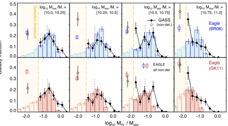
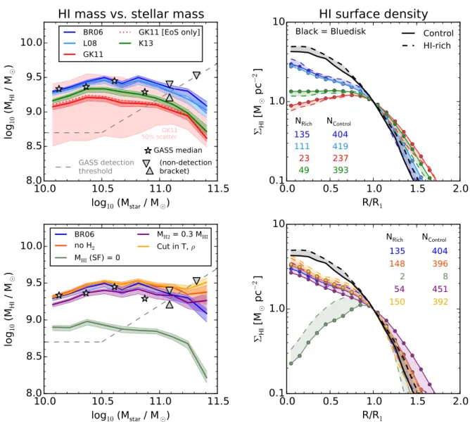
Having established that the neutral hydrogen content of EAGLE galaxies agrees with observations, we now turn to analysing the atomic hydrogen subcomponent. Fig.2presents a comparison of the atomic hydrogen mass fractions,MHI/Mstar in EAGLE with data from the GASS survey (Catinella et al. 2010; see Section 3). We show here the distribution of MHI/Mstar for galaxies in four narrow bins of stellar mass (individual panels, mass increases from left to right). Blue/red histograms show the distribution for simulated EAGLE galaxies: in the top row, we adopt the empirical

BR06formula to account for the presence of H2(blue histograms), while this is achieved following the theoreticalGK11formula in the bottom row (red). In both cases, GASS data are represented by black lines. The vertical orange dash–dotted line marks the (maximum) GASS detection threshold in each stellar mass bin: for consistency, we combine all galaxies withMHI/Mstarlower than this into a single ‘non-detected’ bin (blue/red open square and black open diamond in the shaded region on the left).

Figure 2. Comparison of the HImass of EAGLE galaxies (blue/red histograms) with GASS observations (black lines); both samples include only central galaxies. In the top panel, the presence of H2in EAGLE is accounted for with the empirical Blitz & Rosolowski (2006) pressure-law prescription, while the bottom panel shows the corresponding results from the theoretical Gnedin & Kravtsov (2011) partition formula. The shaded region on the left is below the (maximum) GASS detection threshold in each panel; all simulated galaxies in this regime (light blue/red) are combined into the blue/red open square for comparison to the observations. Vertical black (blue/red) dotted lines indicate the median HImass fraction of all GASS (EAGLE) galaxies per stellar mass bin; in the third panel of the top row both lie on top of each other. Error bars show statistical Poisson uncertainties. Both H2prescriptions lead to broad agreement of the predicted HImasses with observations, but the detailed match is considerably better for the Blitz & Rosolowski (2006) H2formula (top).

obtained by other recent hydrodynamic simulations (e.g. Aumer et al.2013, whose HIfractions are higher than observed by∼0.5 dex; see Wang et al. 2014). In contrast, the median HIfraction obtained with the theoretical GK11approach is consistently too low by∼0.1–0.4 dex.

It is possible that the differences between these two H2schemes are driven by inaccurate gas-phase metallicities in EAGLE galaxies, to which the BR06 pressure law is by construction insensitive; further work is required to test whether this is indeed the case. It is also important to keep in mind that dense gas is modelled in a highly simplified way in EAGLE, with the primary aim of circumventing numerical problems that would arise if gas were allowed to cool below∼104_{K at the resolution of EAGLE (see e.g. Schaye & Dalla} Vecchia2008). It is plausible that theBR06andGK11prescriptions simply reflect this imperfect ISM model in different ways, leading to different predictions about the H2fractions.

As mentioned above, Lagos et al. (2015) obtained good agree-ment between the H2content of EAGLE galaxies and observations with theGK11 prescription, which we find to yield too low HI fractions. The likely reason for this apparent contradiction is that Lagos et al. (2015) focus their analysis on the sub-sample of galax-ies above the COLD GASS detection threshold, and include both centrals and satellites: here on the other hand, we consider cen-trals only and calculate overall medians (from both detections and non-detections). Our results are therefore not directly comparable.

The match to GASS in Fig.2is not quite perfect even with the empiricalBR06model, however: on close inspection, the scatter in MHI at fixedMstar is slightly smaller in EAGLE than GASS,

which manifests itself in a relative deficiency of non-detections (26 per cent versus 42 per cent in the highest stellar mass bin) and very HI-rich galaxies (a difference of−0.15 dex in the 90th percentile ofMHI/Mstarin the highest stellar mass bin). The latter discrepancy is also seen with theGK11H2model, and we confirm in Appendix A1 that it is still present even when we ignore the presence of H2completely and assign all neutral gas as ‘HI’. Although the observational scatter may be overestimated due to uncertainties in the stellar mass measurements, we demonstrate below that a more likely cause is the presence of spuriously large HI holes in the simulated galaxies. Overall, however, we can conclude that (central) EAGLE galaxies acquire approximately realistic amounts of HIby z=0, with only relatively minor uncertainties introduced by the choice of model to account for the presence of H2.

6 T H E I N T E R N A L S T R U C T U R E O F HI I N S I M U L AT E D G A L A X I E S

6.1 Visual inspection of HImorphologies

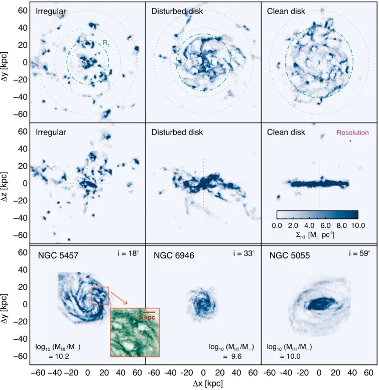
As a first qualitative step, we have created mock HIimages of all simulated galaxies satisfying our selection criteria, by assigning the HImass of particles within a line-of-sight interval of [−70, 70] kpc relative to the galaxy centre to anx×ygrid with pixels of 0.5 kpc, and smoothing with a Gaussian FWHM of 1 kpc. For simplicity, we only do this with the empiricalBR06H2correction. All images were then inspected visually, and the galaxies assigned to one of three broad morphological categories: (a) ‘Irregular’ (no disc-like structure), (b) ‘Disturbed HIdiscs’ (which are not flat when edge-on, and instead show e.g. prominent warps), and (c) ‘Clean HI discs’. Their relative abundances will be discussed in Section 6.2 below. While this is inevitably a subjective classification, it can still offer valuable insight into the HI structure that may not be apparent from a simple quantitative analysis. A typical example galaxy from each category is shown in the first two rows of Fig.3; each has similar total HImass (log10MHI/M =[9.9,10.1]) but rather different appearance. Galaxies have been rotated to face-on in the top row, and to edge-on in the middle; the disc plane is defined to be perpendicular to the angular momentum axis of all HIwithin a spherical 50 kpc aperture which corresponds roughly to the edge of the largest HIdiscs in our sample (see Fig.6below). The scaling is linear from 0 to 10 Mpc−2_{with darker shades of blue indicating} denser gas; the smoothing scale of 1 kpc is indicated with a purple circle in the middle-right panel.

‘Irregular’ galaxies in particular (left-hand panels) typically con-tain a large number of HI‘blobs’ that are typically representing gas in the process of accreting on to the galaxy. Although the ‘disc’ galaxies (middle and right-hand columns) have their HI pre-dominantly in a more or less thin disc, many of these also show pronounced substructure with dense clumps as well as large (∼10– 20 kpc) HIholes. To illustrate the varying degree to which the latter are apparent in different galaxies, we show in Fig.4mock face-on HIimages of three galaxies: one with clearly visible holes (left), one with only tentative hole identifications (middle), and one without visible large holes (right).

We have verified that these holes are also found in the total gas density maps, so they are not an artefact of our HImodelling (i.e. they are not regions where most of the neutral gas is H2). From inspection of the high time resolution ‘snipshot’ outputs in EAGLE (see Schaye et al.2015), they form rapidly and can reach sizes of∼10 kpc within only 20 Myr. This suggests that they are the result of heating events associated with star formation that are (individually) orders of magnitude more energetic than supernova explosions in the real Universe as a result of the limited resolution of EAGLE. Their detailed formation and survival is almost certainly more complex, however: as we show below, a clear correlation between star formation and occurrence of holes is not observed in the EAGLE galaxies.

For comparison, the bottom row of Fig.3displays three observed HImaps of nearby spiral galaxies of comparableMHI– NGC 5457, NGC 6946, and NGC 5055 – from The HINearby Galaxies Sur-vey (THINGS; Walter et al.2008) smoothed to the same spatial resolution as our simulated maps (1 kpc). These clearly look differ-ent from even the simulated ‘clean disc’ galaxies and have a much smoother but also more intricate structure (see also Braun et al.

2009) with clear spiral arms. This difference in appearance can be attributed to the imperfect modelling of the ISM in EAGLE, which does not explicitly include a cold phase, and must therefore impose a pressure floor for high-density gas (Schaye & Dalla Vecchia2008; Schaye et al.2015). In addition, the observed galaxies do not show

HIholes comparable to those in the simulation, although such fea-tures do occur on smaller scales (Boomsma et al.2008): the small inset in the bottom row shows a zoom of a 20×20 kpc region of the almost face-on galaxy NGC 5457 which clearly shows numerous holes up to scales of∼5 kpc (note that the inset uses a square-root scaling for improved clarity, and is therefore shown in a different colour). Rather than theexistenceof HIholes being an artefact of the simulation, it is rather their size and hence covering fraction in the disc that is in tension with observations.

Another apparent disagreement between the simulations and ob-servations is the thickness of the HIdiscs: as the middle-right panel shows, even a ‘clean disc’ extends several kpc in the vertical direc-tion. The exponential scaleheight of this disc is∼1.5 kpc, several times larger than the values indicated by observations of HIin the Milky Way (Dickey & Lockman1990). We note, however, that this is only a factor of∼2 larger than the gravitational softening length of the simulation, which may largely explain this discrepancy. Another plausible contributor is the imposed temperature floor of∼104_K, which corresponds to a Jeans length of∼1 kpc. It is conceivable that the artificial thickening of the disc and the unrealistically large size of HIholes noted above are in fact related: a thicker disc im-plies a lower volume density and hence less mass swept up per unit distance. Despite these differences in detail, we show below that the azimuthally averaged distribution of HIin our simulated galaxies agrees quantitatively with observations, both in terms of the HIsizes and surface density profiles.

6.2 Correlations of HImorphology with other galaxy properties

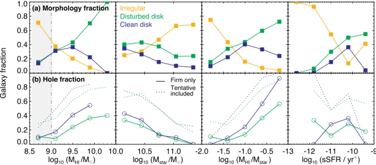
The relative abundance of each morphological type as a function of, respectively, the total HImass, stellar mass, HImass fraction and specific star formation rate (sSFR) is shown in the top panels of Fig.5. HImorphology correlates strongly with all four of these parameters: irregular distributions are most common at low HImass, highMstarand low sSFR, whereas the fraction of discs is highest in the opposite regimes. Interestingly, the fraction ofcleandiscs (blue line in Fig.5) shows no such simple behaviour: they are most common at intermediate MHI≈109.4M, while most galaxies at the highMHIend show a ‘disturbed disc’ morphology. As HI content and sSFR are correlated, it is not surprising to see similar trends with the latter (rightmost panel): the fraction of clean discs drops sharply for the most actively star-forming galaxies.

Note that the left-hand column in particular (trends withMHI) suffers from incompleteness due to our imposed stellar mass thresh-old of Mstar ≥ 1010 M: there is a large population of less massive galaxies, many of which with MHI high enough to fall within the range plotted here. With a median MHI/Mstar=0.1 at Mstar = 1010 M (see Fig. 2), this mostly affects the range MHI109M which is therefore shaded grey in Fig. 5. This should be kept in mind when comparing to HIlimited surveys, but insofar as onlymassivegalaxies are concerned (Mstar≥1010M), it does not affect our results.

Figure 3. Top and middle row: Three typical examples of EAGLE galaxies with different HImorphologies, but similar HImass log10(MH I/M)=[9.9,10.1]: Irregular (left), Disturbed disc (middle) and Clean disc (right). Face-on images are shown in the top row, edge-on equivalents below. For comparison, the bottom row shows three observed HIimages from THINGS (Walter et al.2008) at the same physical scale; these do not correspond to the same morphology categories as the simulated galaxies above. All images use the same linear scaling, as given in the middle-right panel, and are Gaussian-smoothed to a (FWHM) resolution of 1 kpc (purple circle in the middle-right panel). The green dash–dotted rings in the top row show the characteristic radiusR1for each galaxy (see Section 6.3); the grey dotted circles indicate radii of 10, 20, 40, and 60 kpc, respectively. The red dotted ‘cross-hairs’ in the middle row indicate the best-fitting HIdisc plane and axis. The inset in the bottom row shows a 20×20 kpc zoom-in of NGC 5457, revealing HIholes similar to what is seen in EAGLE but on a smaller scale.

(blue). Even though we here show current sSFR – which may well already have been lowered by the presence of low-density holes – we have tested for correlation between holes and star formation in the recent past (as well as total star formation and SFR density), which yields a similar result. This suggests a complex connection between

Figure 4. Examples of simulated face-on galaxy HIimages with clear (left), tentative (middle) and no (right) HIholes as found by visual inspection; all of them have similar HImass. The scaling is the same as in Fig.3. Note that even the ‘no holes’ galaxy in the right-hand panel shows some hole-like structures, but these are much smaller than those seen in the left-hand panel and therefore not classified as ‘holes’ here.

Figure 5. Fraction of galaxies with different HImorphologies (top), and with visible HIholes (bottom, dotted lines include tentative identifications). From left to right, the individual columns show the fractions as a function of HImass, stellar mass, HImass fraction and specific star formation rate (sSFR). The fraction of disturbed discs increases strongly with HImass, in qualitative agreement with observations; the same is true for the fraction of galaxies with visible HIholes. Trends are also seen with the other galaxy parameters, as discussed in the text. The grey region in the left-hand column is affected by our imposed stellar mass limit.

In summary, a large fraction of our simulated galaxies (64 per cent) show a disc morphology of their HIcontent (par-ticularly at highMHI), but nearly two thirds of these are evidently disturbed. All HIdiscs are a factor of several too thick and lack the intricate spiral structure seen in observed HImaps, which is a direct consequence of the simplified ISM modelling in EAGLE. Particu-larly at highMHIand lowMstar, many galaxies furthermore show HIholes that are larger than what is observed (43 and 19 per cent of all central galaxies, respectively, with and without tentative hole identifications).

6.3 HIsize–mass relation

As a simple one-parameter proxy for the internal gas distribution, we next investigate the ‘characteristic’ size of the HIdiscs, which

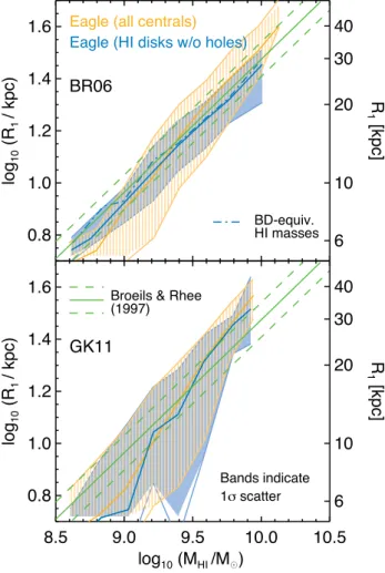
Figure 6. The HImass–size relation for EAGLE galaxies (blue/orange bands), compared to the observational data from Broeils & Rhee (1997) (green lines). Orange includes all (central) EAGLE galaxies whereas blue only includes those with a visually confirmed HIdisc that did not show prominent HIholes. The top panel shows results with the empirical Blitz & Rosolowski (2006) H2model, whereas the theoretical Gnedin & Kravtsov (2011) approach is used in the bottom panel. For the former, the agreement of the median trends is already quite good in the full sample, and even better for the ‘clean’ subset (blue) over more than an order of magnitude in HI mass, especially when using ‘Bluedisk’ equivalent HImasses (dash–dotted line; see text). The theoretical model (bottom) predicts an HImass–size relation that is significantly too steep.

(circular) annuli of width 2.5 kpc.R1is then determined by inter-polating linearly between the outermost bin with density above the threshold of 1 Mpc−2_{, and the one beyond this.}8_{In the top row of} Fig.3,R1is shown as a dark green dash–dotted circle, and coincides approximately with what one would visually identify as the ‘outer edge’ of the HIdisc.

In Fig.6, we show the resulting relation betweenR1andMHI for EAGLE galaxies. As before, we select only central galaxies;9

8_{We note that this procedure is not strictly self-consistent, because such} an interpolation yields, in general, a cumulative mass profile that differs from the true profile. However, we have experimented with more elaborate methods such as linear or quadratic spline fits, or narrower profile bins. None of these alternatives differ substantially from the simple method adopted here.

9_{We have verified that the result is virtually unchanged when potentially} interacting galaxies are excluded, i.e. those where a neighbouring galaxy within 150 kpc has a stellar mass exceeding one tenth of its own.

we show results for both the empiricalBR06(top) and theoretical

GK11prescription (bottom) to account for H2. The running median and 1σscatter (defined as the 15.9/84.1 percentile) of these is shown in orange. To test the influence of HImorphology, we also show (in blue) the size–mass relation for only the subset of simulated galaxies that have been visually classified as containing a well-aligned HIdisc without prominent holes.10 The green solid line represents the best fit of Broeils & Rhee (1997), with 1σ standard deviation indicated by the green dashed lines (note that our plot has thex- andy-axes swapped relative to their fig. 4, and that they show

D1≡2R1instead).

In general, the EAGLE galaxies follow the observed relation quite well. The full sample (orange) has a slope that is some-what steeper than observed with both H2 recipes (0.59 versus 0.51, i.e. a 16 per cent difference with BR06, and 52 per cent with GK11). With the empirical BR06 method (top), the ‘disc-only, no holes’ distribution (blue) agrees with the observations to better than 0.1 dex over the full range ofMHI that we probe here, log₁₀(MHI/M)=[8.5,10.0]. The agreement gets better still when we calculate the HImasses in analogy to the Bluedisk survey (see below), the observations for which were also conducted at the WSRT: this reducesMHIslightly at the low-MHIend (see top panel of Fig.A2) and therefore improves the agreement of EAGLE with the Broeils & Rhee (1997) relation to<0.05 dex. We note, however, that Broeils & van Woerden (1994) find close agreement between the interferometry-derived HImasses used by Broeils & Rhee (1997) and single-dish measurements, so it is not clear whether this is indeed a more fair comparison to the data. We also note that the scatter in the overall EAGLE sample is somewhat too large, by a factor of∼2. Again, the agreement here is better in the sample that excludes galaxies with prominent HIholes (blue). With theGK11 H2formula (bottom), excluding holes makes no appreciable differ-ence, and the HIsize–mass relation remains steeper and broader than observed.

6.4 Density profiles for HI-rich and ‘normal’ galaxies

A more detailed quantitative test of the HIstructure is to compare the radial (surface) density profiles to observations. A particularly inter-esting question in this respect is how atypically HI-rich galaxies – which have likely been particularly efficient at accreting HIrecently – compare to those with average HIcontent. Motivated by this con-sideration, the Bluedisk survey (Wang et al.2013) has recently observed a set of 25 galaxies expected to be HI-rich, and a similar number of ‘control’ galaxies, generating resolved HImaps with a resolution of∼10 kpc. One key discovery of this study has been that the HIsurface density profiles ofallgalaxies, both HI-rich and normal, follow a ‘universal’ shape as long as they are normalized by the characteristic HIdisc sizeR1(Wang et al.2014). We will now compare the EAGLE galaxies to these observations. For sim-plicity, we focus first on results obtained with the empiricalBR06

H2model which, as shown above, leads to total HImasses in good agreement with observations. Profiles obtained with the theoretical H2formula ofGK11will be presented in Section 6.4.3 below.

6.4.1 Sample definitions

From our 2083 central EAGLE galaxies with log10(Mstar/M)= [10.0, 11.0] – the same range as in Bluedisk – we select those

with a Petrosian half-light radiusR50,z ≥ 3 kpc. This radius is defined as enclosing 50 per cent of the Petrosian flux in the SDSSz -band11_{obtained from stellar population synthesis (SPS) modelling} (Trayford et al.2015). As we show in Appendix C1, this simple size cut approximately reproduces the more complex original sample selection in the Bluedisk survey (Wang et al.2013). We have verified that the profiles shown below are insensitive to the exact value of the size cut, and are actually almost unchanged when all galaxies are included, regardless of size.

This simulated sample with 607 members is then divided into ‘HI-rich’ galaxies withMHI≥109.8M, and a ‘control’ sample with 109.1_M

≤MHI≤109.8M. As opposed to an – equally plausible – set of cuts inMHI/Mstar, these limits approximately correspond to the sample division in Bluedisk (see Wang et al.

2013and Appendix C2). For consistency with the observations, we calculate HImasses here in a ‘Bluedisk-equivalent’ fashion (Wang et al.2013): a two-dimensional HIsurface density map with pixel size 0.5 kpc was created (with the simulationz-coordinate as the line of sight, i.e. random galaxy orientations) and then smoothed with an elliptical Gaussian of FWHM=14 (9) kpc major (minor) axes. This corresponds approximately to the WSRT beam size at the median redshift of the Bluedisk galaxies (˜z≈0.027). From these maps, we then sum over all pixels withHIabove the median Bluedisk detection threshold of 4.6×1019_{atoms cm}−2_{(=0.37 M}

pc−2_in HI) to obtain the total HImass of the galaxy. In Appendix A2, we show that the resultingMHIare typically less than 0.1 dex below the ‘GASS-equivalent’ mass forMHI≥109.1M.

Recall from Section 5 that EAGLE has a deficiency of galaxies at the HI-rich end. This is unfortunate for the present purpose, because it means that our simulated HI-rich galaxies are typically not quite as extreme as those in the corresponding Bluedisk sample. How-ever, the two populations are still clearly different and enable us to test the universality of the HIdensity profile: The 406 simulated ‘control’ galaxies have a median log10(MHI/M)=9.61, whereas the 133 ‘HI-rich’ counterparts12have a median log₁₀(MHI/M)= 9.93. For comparison, the Bluedisk HI-rich galaxies have a me-dian log₁₀(MHI/M)=10.09 (N= 23) and the control sample log10(MHI/M)=9.59 (N=18). The difference between the two EAGLE samples (0.32 dex) is therefore approximately two thirds of that in Bluedisk (0.5 dex).

6.4.2 Density profile comparison

In Wang et al. (2014), density profiles were extracted using elliptical annuli with orientation and axis ratio (b/a) taken from the best-fitting ellipse to the stellarr-band light, and then multiplied by a factor ofb/a≈cos (θ) to correct the profiles to face-on. For the analysis of our simulated galaxies, we simply rotate them to face-on by aligning the angular momentum axis of the HIin the central 50 kpc with the line of sight (as in Fig.3). For each galaxy, an HI image was then created as described above, and the surface density

11_{As detailed in Appendix C1, the radiiR}

50,zobtained for our simulated galaxies are systematically too large compared to observations from SDSS; this is investigated in more detail by Furlong et al. (2015b). For our pur-pose, we simply re-scale the distribution ofR50,zto enforce a match to the observational data. This ad hoc fix does not invalidate our results below, because we are only concerned with relative size comparisons, and only use the stellar sizes to select the overall sample to compare to Bluedisk. 12_{There are some additional galaxies withM}

H I<109.1M, which are not included in either sample.

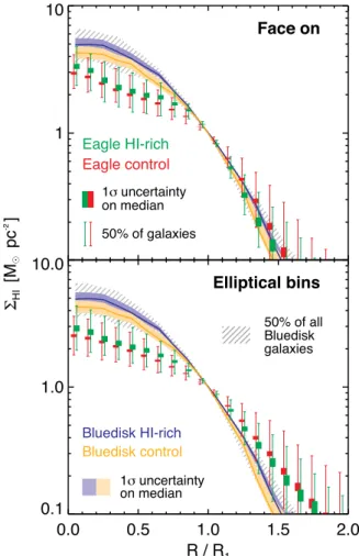
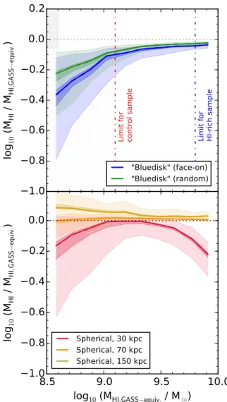
Figure 7. The scaled HIsurface density profiles for galaxies in the EAGLE simulation (red/green rectangles) and in the Bluedisk survey (yellow/blue shaded bands). Galaxies are split into ‘HI-rich’ and ‘control’ samples based on their HImass, as explained in the text. The Bluedisk profiles are identical in both panels, but different methods are applied to EAGLE: Top: galaxies are rotated to face-on. Bottom: profiles are extracted in random orientation in elliptical bins with position angle and axis ratio determined from the stellarr -band light (as in the Bluedisk analysis). In agreement with observations, both methods yield similar profiles for simulated HI-rich and control galaxies. However, the EAGLE profiles deviate from the observations in the central region, and with the ‘elliptical bin’ inclination correction (bottom), they are also too shallow in the outskirts.

profile extracted with 20 equally spaced bins from 0 to 2R1(recall that R1 is defined as the radius at which the HI surface density drops to 1 Mpc−2_{). Galaxies were then median-stacked to obtain} the average profile for the HI-rich and control galaxies. The same procedure was applied to the Bluedisk profiles from Wang et al. (2014).

The result is shown in the top panel of Fig.7. Yellow and blue lines trace the median profiles for HI-rich and control galaxies in Bluedisk. As in Fig. 1, shaded bands indicate the statistical 1σ uncertainty on the median, i.e. they extend fromσlowtoσhighwhere σlow (high)=˜HI+(P15.9 (84.1)−˜HI)/

√

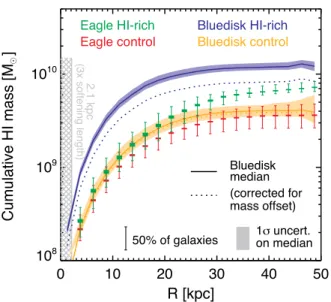
Figure 8. Cumulative HImass profiles for EAGLE galaxies (green/red) compared to observations from Bluedisk (blue/yellow); different colours denote control/HI-rich galaxies as in Fig.7, but here thex-axis is not nor-malized byR1. For Bluedisk, dotted lines show the profiles corrected for the offset in total HImass in each sample relative to EAGLE (see text). Bands and thick boxes indicate the 1σ uncertainty on the median. There is a clear lack of HIin the central region (R20 kpc) in EAGLE, which manifests itself in the lower-than-observed HImasses of HI-rich galaxies (blue/green). For the ‘control’ sample, the HIdeficit in the centre is largely compensated by the slightly too shallow decline of the profile in the outer parts (yellow/red).

and by the grey hatched region for Bluedisk, both of which show the interval occupied by 50 per cent of galaxies (i.e.P25toP75).

In the outer region (RR1), simulated and observed profiles gen-erally agree to within the statistical uncertainties. Both simulated control and HI-rich galaxies follow an exponential profile (straight line in the log-linear plot), although the gradient is slightly steeper for the HI-rich galaxies (green, discrepancy at∼2σ level). The observed galaxy profiles show an approximately equal, but oppo-site difference (steeper profiles for control galaxies), although the small number of Bluedisk galaxies means that this difference is not statistically significant.

In the inner parts (RR1), there is a much more pronounced dis-crepancy between simulations and observations: the former ‘under-cut’ the observed profile. Interestingly, the simulated HI-rich and control profiles are still almost identical, to within<0.1 dex (with a minor excess, significant at∼2σ, in HI-rich galaxies, as in ob-servations). To test whether this is a result of the slightly different analysis for the simulated and observed galaxies, we have repro-duced the Bluedisk analysis on our simulated galaxies exactly (i.e. we extracted the profiles in elliptical rings with position angle and axis ratio given by the stellarrband, and multiplied with a correc-tion factor ofb/a), the result of which is shown in the bottom panel of Fig.7. However, this fails to ameliorate the tension in the central region, and adds another disagreement in the outer parts, where the simulated profiles are now far too shallow; we shall return to this shortly.

It is worth keeping in mind that, due to the scaling of thex-axis in Fig.7byR1, one cannot directly infer the actual mass distribu-tion from the profiles. We therefore explicitly show a comparison between the cumulative mass profiles in EAGLE and Bluedisk in Fig.8; the symbols have the same meaning as in Fig.7with the addi-tion of the grey hatched region denoting the (small) zone influenced

by resolution effects (R≤3, the gravitational softening length). Note that thex-axis here shows the actual galactocentric radiusRin kpc, and is not normalized byR1. As expected, simulated galaxies show a deficit of mass in the inner region (R30 kpc). However, for the control galaxies (red) this is almost completely compensated by the outer parts, where the surface density profile is slightly too shallow. In the HI-rich sample, on the other hand, the central deficit manifests itself in a lower total HImass in simulated galaxies, as already seen in Fig.2. To confirm that this interpretation also holds quantitatively, the dashed lines in Fig.8show the Bluedisk profiles re-scaled by the ratio of median totalMHIin EAGLE and Bluedisk, 0.95 and 0.69, respectively, for the HI-rich and control samples. As expected, this shows much better agreement with the simulated HI -rich profile atRR1. The lack of extremely HI-massive galaxies in EAGLE is therefore directly connected to the missing HIin the central galaxy regions.

6.4.3 Why are the simulated profiles different from observations?

We are therefore faced with two puzzles: (i) Why does the in-clination correction through elliptical bins work so poorly for the outskirts of the simulated galaxies? (ii) Why is the HIdensity too low in the inner regions of simulated galaxies?

For the first question, one natural explanation might be that the inclination of the HIdisc does not correspond exactly to the elliptic-ity of ther-band light (e.g. Serra et al.2012; Wang et al.2013). We test this in Appendix D and there is indeed good evidence that this is the case: observationally, the distribution ofb/ain the Bluedisk sample is far from flat, with a deficit at both small (b/a0.3) and high (b/a0.9) axis ratios, which is in conflict with the simple assumption cosθ = b/abecause the distribution of cosθ should be uniform. Likewise, a direct comparison between the inclination angle and stellarb/ain EAGLE shows both significant scatter and a systematic offset for galaxies withb/a0.6. However, we have repeated the ‘elliptical bin’ analysis on our simulated galaxies, with axis ratio and orientation angle derived directly from the orientation of the HIangular momentum axis instead of fits to the stellar light, and the resulting profiles are almost identical to those shown in the bottom panel of Fig.7.

There must therefore be a genuine difference between the simu-lated and observed galaxies, and one obvious candidate for this is the artificially increased thickness of the HIdisc in EAGLE (see discussion in Section 6.1), which may lead the elliptical-bin incli-nation correction, based on an infinitesimally thin HIdisc, to fail. Any line of sight will intersect a thick disc not only at one point, but over a finite interval, which effectively smears out the resulting profile: an inclined line of sight that intersects the disc mid-plane in the galaxy outskirts (at a radiusRa) will actually pick up most

HIatR<Rawhere the HIdensity is higher, thus leading to a

shal-lower outer profile. By conservation of total mass, the density must appear lower in the inner regions, exactly as seen in Fig.7. This interpretation would also explain why the (outer) face-on profiles in EAGLE are still a good match to observations, because they are by definition insensitive to the vertical structure of the HIdiscs.

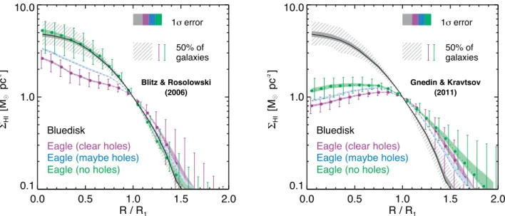
Figure 9. Dependence of HIsurface density profiles on the presence of visible HIholes. The left-hand panel shows results obtained with the empirical Blitz & Rosolowski (2006) H2model, whereas the theoretical Gnedin & Kravtsov (2011) formula is used in the right-hand panel. Green points show the profile for galaxies with no visual evidence of holes, while purple points show those galaxies where holes are clearly visible. Galaxies with tentative hole detections are shown in blue; for clarity we have omitted the error bars here. With the empirical H2formula (left), the hole-free sample (green) is in good agreement with the Bluedisk data over the entire radial range we probe here, while galaxies with hole detections show a deficit in the central HIprofile. Using the theoretical formula from Gnedin & Kravtsov (2011), galaxies with and without holes have centralH Iprofiles that are significantly too low compared to observations.

therefore be regarded as truly face-on, and the comparison to the face-on profiles from EAGLE in the top panel of Fig.7as the most meaningful test of the simulated HIsurface density profiles.

The discrepancy in thecentralregions must have a different ori-gin, as it is present in both the face-on and elliptical-bin-corrected profiles. One possibility here is that this is related to the spurious HIholes that we had already noted in the discussion of Fig.3. To test this hypothesis, we show in Fig.9the median-stacked profiles (now again normalized byR1) for galaxies with clear visual hole detections (purple), as well as those without (green) and those with tentative-only identifications (blue). For simplicity, we here com-bine HI-rich and control galaxies. The left-hand panel shows the profiles obtained with the empiricalBR06pressure-law to account for the presence of H2; for comparison we also show the equivalent profiles obtained when using the theoreticalGK11formula in the right-hand panel. In both cases, the observed profile from Bluedisk (HI-rich and control combined) is shown in black.

It is evident that the discrepancy in the inner region seen with the BR06 model as discussed above is indeed connected to the presence of HIholes. Simulated galaxies without holes (green) fol-low the observed profile almost exactly over the entire radial range that we consider here (discrepancy< 0.07 dex). The scatter re-mains slightly larger than in the observations, but only by typically

50 per cent. In contrast, galaxies with clearly visible holes (pur-ple) have a much shallower central profile (by up to a factor of∼2), with tentative identifications (blue) lying in-between. It is worth pointing out that the ‘hole’ and ‘no-hole’ populations have profiles that differ by more than the typical scatter in each: there is a clear difference betweenindividualgalaxies in the two categories, and not just in a statistical sense.

Although smaller, there is also a slight effect in the outer profiles where the HIsurface density is slightly higher in galaxies with holes than without (by0.1 dex). This may seem counter-intuitive, but is explained by the fact that the profiles are scaled byR1which is affected by the presence of holes as well (see Fig.6). It is, of course, no surprise that galaxies with holes lack HIand therefore

show shallower inner profiles than those without visible evidence for them. What is far less trivial, however, is that the ‘hole-free’ sample agrees so well with the observations:the discrepancy in the surface density profiles between EAGLE and Bluedisk can thus be fully attributed to the existence of these holes.

TheGK11profiles (right-hand panel of Fig.9) show a similar general trend – a higher central HIsurface density for hole-free galaxies – but the difference is much smaller here than with the

BR06 formula. Moreover, all three profiles are significantly too low withinR1, with a discrepancy by a factor of5 in the very centre. Evidently, the theoretically basedGK11formula assigns an unphysically large fraction of the neutral gas in the central EAGLE galaxy regions as H2, which would explain why theGK11total HI masses as shown in Fig.2are biased low. In addition, theouter

HIprofiles are actually slightly more discrepant (i.e. shallower) for hole-free galaxies than those with holes, indicating that the normalization radiusR1is somewhat too small at fixedMstar(see also Fig.6). The lack of HI in the central region also explains the smaller effect of holes, compared toBR06: there is simply not enough HIeven in hole-free galaxies for these features to have a significant impact.

We note that it is, in principle, conceivable that the profile agree-ment between HI-rich and control galaxies is not actually a physical feature, but rather a result of the comparatively large beam size: re-call that the HImaps from EAGLE had been artificially reduced in resolution to the same level as in Bluedisk. However, we explic-itly check for this in Appendix E, where we calculate the EAGLE HIsurface density profiles from higher-resolution maps. Although the detailed shape of the profiles does indeed vary with the beam size, the close agreement between HI-rich and control galaxies re-mains. This strongly suggests that it is a genuine physical feature of the simulated – and observed – galaxies, rather than a smoothing artefact.