Efficient
ℓ
0-Norm Feature Selection Based on Augmented and
Penalized Minimization
Xiang Lic, Shanghong Xiea, Donglin Zengb, and Yuanjia Wanga,*,†
aDepartment of Biostatistics, Mailman School of Public Health, Columbia University, New York,
NY 10032, U.S.A
bDepartment of Biostatistics, University of North Carolina, Chapel Hill, North Carolina 27599,
U.S.A
cStatistics and Decision Sciences, Janssen Research & Development, LLC, Raritan, NJ, U.S.A
Abstract
Advances in high-throughput technologies in genomics and imaging yield unprecedentedly large numbers of prognostic biomarkers. To accommodate the scale of biomarkers and study their association with disease outcomes, penalized regression is often used to identify important biomarkers. The ideal variable selection procedure would search for the best subset of predictors, which is equivalent to imposing an ℓ0-penalty on the regression coefficients. Since this
optimization is a non-deterministic polynomial-time hard (NP-hard) problem that does not scale with number of biomarkers, alternative methods mostly place smooth penalties on the regression parameters, which lead to computationally feasible optimization problems. However, empirical studies and theoretical analyses show that convex approximation of ℓ0-norm (e.g., ℓ1) does not outperform their ℓ0 counterpart. The progress for ℓ0-norm feature selection is relatively slower, where the main methods are greedy algorithms such as stepwise regression or orthogonal
matching pursuit. Penalized regression based on regularizing ℓ0-norm remains much less explored in the literature. In this work, inspired by the recently popular augmenting and data splitting algorithms including alternating direction method of multipliers, we propose a two-stage procedure for ℓ0-penalty variable selection, referred to as augmented penalized minimization-L0 (APM-L0). APM-L0 targets ℓ0-norm as closely as possible while keeping computation tractable, efficient, and simple, which is achieved by iterating between a convex regularized regression and a simple hard-thresholding estimation. The procedure can be viewed as arising from regularized optimization with truncated ℓ1 norm. Thus, we propose to treat regularization parameter and thresholding parameter as tuning parameters and select based on cross-validation. A one-step coordinate descent algorithm is used in the first stage to significantly improve computational efficiency. Through extensive simulation studies and real data application, we demonstrate superior performance of the proposed method in terms of selection accuracy and computational speed as compared to existing methods. The proposed APM-L0 procedure is implemented in the R-package APML0.
*Correspondence to: Yuanjia Wang, Department of Biostatistics, Mailman School of Public Health, Columbia University, New York,
HHS Public Access
Author manuscript
Stat Med
. Author manuscript; available in PMC 2019 February 10.Published in final edited form as:
Stat Med. 2018 February 10; 37(3): 473–486. doi:10.1002/sim.7526.
A
uthor Man
uscr
ipt
A
uthor Man
uscr
ipt
A
uthor Man
uscr
ipt
A
uthor Man
uscr
Keywords
ADMM; Variable Selection; ℓ0-Penalty; Censored Data; Biomarker Signature
1. Introduction
Recent advances in high-throughput technologies in genomics and imaging yield unprecedentedly large numbers of prognostic biomarkers to be examined. The curse of dimensionality poses challenges for the traditional regression analysis when studying association between high-dimensional biomarkers and disease outcomes [1]. To cope with the scale of the number of variables, many regularized methods, which introduce sparsity penalties to the regression models or likelihood functions, have been developed for simultaneous parameter estimation and variable selection [2–7]. The most ideal penalty for the variable selection purpose is the ℓ0-norm of the regression coefficients for all predictors, which is equivalent to the number of non-zero terms among the coefficients, and also referred to as the best subset selection. Unfortunately, due to the non-convexity and discontinuity of the ℓ0-norm, solving such a regularized optimization is computationally challenging, known as non-deterministic polynomial-time hard (NP-hard) [8]. Instead, other continuous or smooth penalties have been suggested in different contexts [2–7]. Particularly, the convex penalty based on the ℓ1-norm [2, 3], ℓ2-norm, or their combination [4, 5] was introduced as a relaxation of ℓ0-norm, providing a computationally attractive regularization form.
Alternative approaches based on non-convex penalties such as smoothly clipped absolute deviation (SCAD) [9, 10] and approximate ℓ0-penalty [11, 12] apply less shrinkage on large coefficients and hence reduce the estimation bias. Moreover, non-convex penalties may yield the property of oracle variable selection in the large sample sense. However, one difficulty of using non-convex penalties is computational instability and sensitivity to initial values. None of these methods directly use the ℓ0-penalty, and thus likely will still include some variables with small effects in the final model, especially under the high-dimensional data framework with large p and small n. For example, Lin et al. [13] showed that ℓ1-regularized methods never outperform their ℓ0 counterpart, and may be much worse in some cases. Advancement for ℓ0-norm feature selection is low, where the main methods are greedy algorithms such as stepwise regression or orthogonal matching pursuit [14]. Penalized regression based on regularizing ℓ0-norm remains much less explored in the literature. The penalty function proposed in [15] targets ℓ0-norm but involves heavy computation and non-convex optimization.
To address gaps in knowledge, we propose an efficient two-stage method that aims to regularize ℓ0-norm as close as possible and can be solved by a highly efficient and simple computational algorithm. Our method shares two features with the recently popular alternating direction method of multipliers (ADMM) algorithm [16]: (1) introducing surrogate parameters to augment the original model space; and (2) updating original parameters and surrogate parameters with iteratively alternating optimization. To describe the difference with the ADMM, note that it solves optimization problems of the form
A
uthor Man
uscr
ipt
A
uthor Man
uscr
ipt
A
uthor Man
uscr
ipt
A
uthor Man
uscr
where all f(β) and g(θ) are convex functions. However, a fundamental difference is that g(θ) is the ℓ0-norm of θ in our method, so it is non-convex. Using ℓ0-norm, our variable selection retains an authentic sparsity penalty. Another difference is that the ADMM obtains step sizes for parameter updates as solutions to the Lagrange equations. However, we can regard our soft-thresholding followed by hard-thresholding procedure as arising from a truncated ℓ1 -penalty function and treat step sizes as tuning parameters. Thus, we will use cross-validation instead of Lagrange equations to determine their values, and our tuning parameters are chosen adaptively to the data at hand.
We refer to our method as the augmented penalized minimization (APM-L0). Specifically, APM-L0 iterates between a commonly used regularized regression step and a hard-thresholding estimation step, which can avoid the computational challenges encountered in the ℓ0-regularization problems. To implement APM-L0, we develop a one-step coordinate descent algorithm taking into account the sparsity structure, which results in both significant reduction in memory usage and high efficiency in computation. Furthermore, we propose to simultaneously tune the regularization parameters in both steps based on cross-validation. The method is flexible enough to handle a variety of models (e.g., linear model, logistic model, or Cox proportional hazards model [17]) and structure among variables by imposing a Laplacian penalty [6, 18]. We demonstrate better estimation accuracy, much improved model sparsity, and reduced computational burden over the commonly used ℓ1-type penalties via extensive simulation studies. We provide real data analyses to demonstrate the practical applicability of APM-L0. Lastly, a publicly available R-package APML0 is provided and shown via simulations to speed up computation faster than the commonly used R-package glmnet [19].
The rest of this article is organized as follows. In Section 2, we describe the ℓ0-penalized problems and present the details of APM-L0 approach. We also describe an efficient one-step coordinate descent algorithm for the implementation. In Section 3, we first evaluate the estimation and selection performance of our method and show large efficiency gain in simulation studies. In Section 4, we apply APM-L0 to a real world example: a recently completed comprehensive study on Huntington’s disease (HD), PREDICT-HD [20], where the whole brain structural magnetic resonance imaging (MRI) measures are used to estimate a network regularized biomarker signature for the age-at-onset of HD. Lastly, we conclude with a few remarks in Section 5.
2. Methods and Computational Algorithm
2.1. Regression Model with ℓ0-Penalty
Let β denote a vector of coefficients in a regression model and let l(β) denote a log-likelihood function chosen appropriately depending on the outcome. For example, for continuous outcomes, l(β) is based on linear regression model; and for censored outcomes, l(β) is based on the partial likelihood under the Cox proportional hazards model [17] (details
A
uthor Man
uscr
ipt
A
uthor Man
uscr
ipt
A
uthor Man
uscr
ipt
A
uthor Man
uscr
in Section 2.5). With a large number of biomarkers including genomic and imaging features, directly maximizing l(β) may not be feasible and it is necessary to impose regularization and perform variable selection. The ideal but computationally infeasible feature selection is the best subset selection, that is, performing a regularized regression imposing penalty on the ℓ0 -norm of coefficients:
(1)
where and βj is the jth component of β.
However, due to the non-convexity of the ℓ0-norm, it is difficult to solve (1) with the penalty function p(β) = ρ||β||0, computationally known as NP-hard: in order to select the best subset of non-zero coefficients, we need to evaluate all the possible combinatorial subsets, which grows exponentially with the number of covariates. Existing approaches based on more continuous penalty functions (e.g., ℓ1-, ℓq-norm instead of ℓ0-norm) may often select many non-zero β’s with small magnitude, which leads to a non-parsimonious model and inferior prediction on independent data due to overfitting, a common challenge for high-dimensional data analysis with large p and small n.
Remark—In some applications, components of biomarker variables X exhibit correlation
structure (e.g., correlated gene expressions or brain imaging region of interest (ROI) measures). Such correlation can be naturally described by a network structure through a Laplacian matrix L associated with the network graph. For example, Li and Li [6] and Huang et al. [18] discussed incorporating such a Laplacian quadratic penalty βTLβ into the log-likelihood to perform network-regularized variable selection. This penalty encourages smoothness of the coefficients of predictors that are linked on the network. To accommodate network-informed penalty function, the first term in (1) can be expanded to −n−1l(β) +
ρ2βTLβ by taking into account such a network structure, where ρ2 is a tuning parameter for the Laplacian prior and is selected by cross-validation.
2.2. APM-L0 for the ℓ0-Penalized Variable Selection
Our proposed computational method to solve the NP-hard problem (1), APM-L0, is motivated by a class of proximal methods performing augmentation and splitting, including the ADMM. In a nutshell, APM-L0 is a two-stage iterative procedure where the first stage solves a regularized regression with computationally tractable penalty function, and the second stage performs hard-thresholding. The procedure is simple and highly
computationally efficient. To illustrate the method, we re-formulate the objective function (1) by augmenting the ℓ0-norm of β with a surrogate parameter θ and bound the difference by a smooth convex function which guarantees convergence in the proximal of β:
(2)
A
uthor Man
uscr
ipt
A
uthor Man
uscr
ipt
A
uthor Man
uscr
ipt
A
uthor Man
uscr
where ϕj(x) is a convex function satisfying ϕj(0) = 0 and ϕj(|x|) ≥ 0 for x ≠ 0, and c ≥ 0 is a tuning parameter. A common choice for ϕj(| · |) is the ℓ2-norm, where ϕj(|x|) = x2, j = 1, · · ·, p. Denote by λ a penalty parameter (λ > 0). The Lagrangian form for (2) becomes
(3)
To minimize (3) for a given λ, APM-L0 iteratively update all parameters using the following algorithm: at the kth iteration,
(4)
(5)
where the superscript is the iteration counter. The algorithm is iterated until convergence.
Note that the above update equation (4) is similar to updating a regularized regression. For
(5), it is clear that minimization is performed component-wise. Hence, if , then
; otherwise, the optimal solution is either or depending on
whether is larger than ρ/λ. That is, for j = 1, · · ·, p,
(6)
It can be seen from (6) that the ℓ0-penalty works as hard-thresholding the estimates obtained from the regularized regression in the first step in (4). Many convex penalties proposed in the literature are good choices of ϕj(·), including ℓ1-penalty [2, 3], elastic net (a combination of ℓ1- and ℓ2-penalty) [4, 21], group Lasso [22] and sparse group Lasso [23].
In summary, the APM-L0 approximates solutions to (1) via an ADMM-inspired iterative two-stage method. The first stage replaces ℓ0 penalty with another penalty function that provides computationally tractable optimization, and the second stage corresponds to hard-thresholding. From another view, the APM-L0 performs best subset selection based on the magnitude of β estimated from a regularized regression. By making use of the order and magnitude of β, one can greatly reduce the computing time to evaluate ℓ0-norm.
A
uthor Man
uscr
ipt
A
uthor Man
uscr
ipt
A
uthor Man
uscr
ipt
A
uthor Man
uscr
2.3. Efficient Computation in the First Stage
When there is no closed form solution for the score function of a penalized regression (e.g., in a Cox proportional hazards regression), we can apply a quadratic approximation [5] at some point of the current estimate of β (details in Section 2.5). Previous algorithms such as [19] cyclically updated β̂j, j = 1, · · ·, p, until some convergence criterion was met at the local point β̃. Here, instead of [19], we take a one-step coordinate descent approach to update β̂j only. Our one-step algorithm substantially improves computational efficiency. For the jth component of β̂, we solve
(7)
where l(β|β̂−j) is the log-likelihood function with all the components fixed except the jth component, βj. Furthermore, we construct an active set = {j: β̂j ≠ 0} at the outset and update those β̂j for j ∈ only, which is efficient for handling sparse β by reducing the number of updates. Let η = (η1, · · ·, ηn)T = (βTX1, · · ·, βTXn)T = Xβ. The APM-L0 algorithm is
1. (Initialization) Set β̂ = η̂ = 0 and = ∅.
2. (Active set) Update at β̂.
3. (Loop) Iterate until convergence of β̂: cyclically update β̂j by (7) for j ∈ .
4. Converge if no update of ; otherwise, go to Step 3 with the updated .
When evaluating for a path of λ, we use the previous estimate β̂ and active set as a warm start for the next λ and follow Steps 2–4.
Remark—For a network graph-constrained log-likelihood, the Laplacian matrix L is often
sparse. Hence, in the implementation, we use a sparse matrix to represent L, which greatly reduces memory usage and enhances computational efficiency.
2.4. Simultaneous Selection of Tuning Parameters
An intuitive understanding of APM-L0 is to iteratively carry out (a) regularized regression as laid out in the previous section, and (b) perform hard-thresholding. The tuning parameter λ controls the degree of regularization for the estimators, and the ratio between ρ and λ determines the number of non-null coefficients (sparsity of the model).
In some cases, the ADMM algorithm can be slow to converge. The original ADMM iteratively updates the Lagrangian multiplier λ as, at the kth iteration,
A
uthor Man
uscr
ipt
A
uthor Man
uscr
ipt
A
uthor Man
uscr
ipt
A
uthor Man
uscr
where ak > 0 is a step size. The ak needs to be appropriately chosen to ensure the dual function, defined as g(λ) = infβ,θ Lλ(β, θ), is increasing. Based on the dual optimal λ* obtained by maximizing g(λ), we can recover the primal optimal estimates β* and θ*.
Instead of iteratively updating β, θ and λ, we propose to treat λ as a tuning parameter and search over a set of grid points of λ. At each fixed value of λ, we update β̂ and θ̂ based on the optimization problems (4) and (5). To save computational time, we advocate one iteration update for β and θ, and declare θ̂ as our final estimate. Hence, it is feasible that the algorithm to solve the ℓ0-penalty runs as fast as other regularized regressions (e.g., ℓ1 -penalized regression). Thus, given λ and ρ, our method is implemented in a two-stage fashion:
The path of λ can be set as in Friedman et al. [19]. In the second stage, we arrange |β̂| in decreasing order and directly choose the number of non-null coefficients in β̂ by keeping the
κ largest coefficients of |β̂|. We set the path of κ from zero to the total number of non-null coefficients of β̂. We propose to use cross-validation to simultaneously select both
parameters κ and λ. For example, we suggest to use least squared error for linear regression and partial-likelihood for Cox model [24] as cross-validation criteria.
2.5. Examples of Regression Models and Penalty Functions
We can use any log-concave function/model to replace l(β) in the proposed APM-L0. Let Xi = (Xi1, · · ·, Xip)T denote a vector of covariates and yi be the response variable. For linear regression with continuous outcome, we use
For time-to-event outcomes (e.g., age-at-onset of a disease) subject to independent censoring, we consider Cox model. Let Ti be the time-to-event of interest and Ci be the censoring time. Denote by T̃i = min(Ti, Ci) the observed event time or censoring time and denote by δi = I(Ti ≤ Ci) the event indicator, where I(·) is an indicator function. We use the following log-likelihood function:
A
uthor Man
uscr
ipt
A
uthor Man
uscr
ipt
A
uthor Man
uscr
ipt
A
uthor Man
uscr
where Ri = {k: T̃k ≥ T̃i} denotes the risk set at time T̃i. Because there is no closed form when solving (7), we use the method proposed by Simon et al. [5]. We approximate l(β) based on its second-order Taylor series expansion centered at β̃ (estimated β from the previous iteration) and further approximate the Hessian matrix of l(η) by it’s diagonal matrix to obtain the following function
where
where Cj = {i: T̃i ≤ T̃j}. With little effort, we can extend APM-L0 to other models, such as general linear models. In the subsequent numeric studies, we focus on linear and Cox models.
To reduce the risk of overfitting and incorporate prior biological information, Laplacian penalty is often considered [6] to regularize estimation.
3. Simulation Studies
3.1. Simulation Design and Results
We conducted extensive simulations to evaluate the performance of APM-L0. We chose ϕj(| x|) to be the ℓ1-type penalty function, which provides a computationally attractive form to reduce dimensionality. We compared the proposed method with the commonly used ℓ1-type penalized regressions including Lasso [2, 3], Enet [4, 5], Net and its adaptive version, adaptive network penalty (ANet [6, 7]) for both linear regression and Cox model. For simplicity, we refer to these methods as “ℓ1-type”, to be distinguished from our proposed APM-L0.
To mimic potential correlation between covariates in real world applications, we constructed
X in independent blocks and the nodes within each block were correlated with a correlation
of 0.5. Each block consisted of five nodes and 15 nodes/covariates from three blocks had non-zero effects on the outcome. We fixed the number of covariates in each node at five but varied the total number of covariates, denoted by p. We considered two types of outcome in the simulation, continuous and censored data. For linear regression, we generated
, where βj = (−1)j × 2 exp(−(j − 1)/15) and εi ~ N(0, 1). For Cox model,
A
uthor Man
uscr
ipt
A
uthor Man
uscr
ipt
A
uthor Man
uscr
ipt
A
uthor Man
uscr
the underlying hazard function was given by , where ρ0(t) was specified by a Weibull distribution with shape parameter 5 and scale parameter 2 and βj = (−1)j × 2 exp(−(j − 1)/15). The censoring status was generated from a uniform distribution and randomly assigned to 30% subjects.
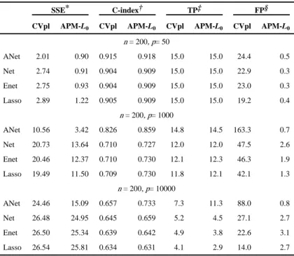
In the simulations, we considered sample size n = 200 with various numbers of covariates. For each simulated dataset, the searching path for λ has a length of 20. Ten-fold cross-validation was applied to choose the optimal tuning parameters. Simulations were repeated 100 times. To evaluate estimation performance, we computed the sum of squared errors (SSE) of the estimated parameters. We also calculated the number of true positive covariates (TP; number of non-null variables correctly selected in the final model) and the number of false positive covariates (FP; number of null variables incorrectly selected in the final model) as measures of the variable selection performance. For the Cox model, we computed the out-sample concordance index (C-index) using 100 random partitions of data into a training set and testing set.
Table 1 summarizes these simulation results. It can be seen from Table 1 that APM-L0 significantly outperforms the commonly used ℓ1-type methods based on cross validation of the partial likelihood (L-CVpl) in terms of both estimation accuracy and selection
performance for all cases. The improvement is substantial with smaller SSE, comparable TP and much less FP for both linear regression and Cox regression. As the number of covariates increases, it becomes more difficult to pick true positive covariates and remove noise covariates. For the setting with small number of covariates where p = 50, both methods are able to select all the true positive covariates but APM-L0 selects 20 times fewer FP than the
ℓ1-type methods. As p increases to 10000, less TP are selected, yielding larger SSE. When p = 10000, the ℓ1-type methods select slightly more TP than APM-L0, but still many more FP, and hence a worse SSE. Comparing different choices of the penalty functions in the first stage ϕj(·) in APM-L0, we find that ANet performs the best since it takes into account of the correlation structure among covariates and adjusts the signs of highly-linked covariates. APM-L0 with Anet penalty gives a higher C-index than CVpl for Cox model when p = 1, 000 or p = 10, 000. The remaining three penalties have similar performance.
We also performed additional simulations with APM-L0 under a fixed λ and number of non-null variables, κ. We fixed λ at 0.01, 0.05, and 0.1 and κ at 10, 20 and 30 and used a Lasso penalty as an example. When comparing APM–L0 with the best scenario of fixing λ and κ, the former yields a higher C-index, a lower number of false positives when p = 50; and gives a slightly lower C-index but less number of false positives when p = 1, 000 or p = 10, 000.
3.2. Running Time
We compared the running time of our R-package APML0 implementing APM-L0 with glmnet [19] under the same parameter settings for various sample sizes and numbers of covariates. As glmnet can only handle Enet and Lasso, the comparison was only performed for these two penalties. To make the algorithms comparable, we generated the path of tuning parameter λ from glmnet and used the same path in the first stage of our method. All calculations were carried out on an Intel Xeon 2.13 GHz processor.
A
uthor Man
uscr
ipt
A
uthor Man
uscr
ipt
A
uthor Man
uscr
ipt
A
uthor Man
uscr
Table 2 shows the running time comparison between APML0 and glmnet. Our
implementation was called from R, and most intensive computation codes were written in C ++ and integrated with R using R-package Rcpp [25]. In Table 2, we observe that APML0 and glmnet have similar running time for linear regression but APML0 runs faster than glmnet for Cox regression. Similar algorithm was used by both packages for linear regression. For Cox model, a quadratic approximation is needed at a local point. APML0 takes one-step coordinate descent at the local point rather than full optimization as done by glmnet. Obtaining high precision of estimates for the intermediate steps is not necessary. Similar idea was adopted in Mittal et al. [26]. Additional simulations with different distribution of covariates, correlations among covariates, and comparison with ADMM are presented in the Appendix.
4. Analysis of Real Data
There is increasing evidence that brain imaging markers are important biomarkers for predicting diagnosis and progression of neurodegenerative disorders [20, 27, 28]. Current work in the clinical literature mostly perform univariate analyses to assess association between individual variables and disease outcome. However, theoretical investigation [2] and various empirical studies [29] suggest that simultaneous approaches based on penalized regressions may avoid overfitting and provide more power than massive univariate
approaches or greedy-search based stepwise regressions. Here, we take a whole-brain approach to evaluate all regional imaging measures simultaneously in predicting age-at-onset (AAO) of Huntington’s disease (HD). Regional brain atrophy measures obtained from structural magnetic resonance imaging (MRI) have been suggested as one of the most robust imaging biomarkers for HD [30]. We analyzed the data from the newly completed
PREDICT-HD study [20] to predict AAO of HD using whole brain subcortical volumetric measures obtained from structural MRI. The regional summary volumetric measures were created by a fully automated procedure and pre-processed using Freesurfer 5.2 (http://
surfer.nmr.mgh.harvard.edu). Details on the imaging marker preprocessing have been
reported previously [20]. Our analysis consists of 840 subjects who were at genetic risk of HD (CAG repeats length ≥36 at the huntingtin gene [31]). The median follow up time was 3 years and 128 subjects developed HD during the study. In our analysis, there were 8 clinical variables (gender, education, baseline total motor score from the UHDRS, and cognitive and functioning measures) and 28 subcortical MRI imaging ROI biomarkers measured at the baseline visit. To account for correlation among imaging measures, elastic net (Enet) penalty and Laplacian penalty was used for the function ϕj(·) in the APM-L0. We used control subjects (no HD mutation, CAG repeats length < 36) in PREDICT-HD to estimate the correlation matrix used in the Laplacian penalty. All variables were standardized before fitting the model.
We compare APM-L0 with the usual penalized regression implemented in glmnet using cross-validation to select tuning parameter (referred to as L-CVpl). To obtain an out-of-sample measure of performance, we randomly partitioned the data into a training set and testing set, where we used the training set to fit the data and testing set to estimate the performance. We used ten-fold cross-validation to select tuning parameter on the training set. Table 3 shows that given a penalty function, the proposed APM-L0 procedure selected
A
uthor Man
uscr
ipt
A
uthor Man
uscr
ipt
A
uthor Man
uscr
ipt
A
uthor Man
uscr
less number of biomarkers than L-CVpl (on average 8.17 variables less under ANet penalty and 4.14 variables less under Lasso penalty), without sacrificing the prediction performance (comparable cross-validated C-index [32], brier score [33], and partial likelihood).
Moreover, APM-L0 under sign-adjusted ANet penalty has higher C-index, lower Brier score and higher partial likelihood than under Lasso penalty. We further show the estimated standardized regression coefficients (effect sizes) in Figure 1 for all four procedures. Comparing APM-L0 with L-CVpl, we see that the former removed several biomarkers with small effects (e.g., Left Lateral Ventricle) which were clearly noise variables from a
biological point of view, while strengthening effects from ROIs such as Putamen, Thalamus, and Palladium. Comparing Lasso penalty with sign-adjusted ANet, we see that the former does not select ROIs shown to be highly predictive in prior literature [20] such as left or right side of Putamen. In addition, ANet can select the linked biomarkers with opposite effects, such as left and right sides of hippocampus, which indicates the necessity of controlling for the direction of association of biomarkers.
Some of the variables selected by APM-L0 are consistent with previously identified in the literature [20] from the PREDICT-HD study. However, previous literature did not take a multivariate approach so that the relative ranking of biomarkers’ ability to predict HD onset in a multivariate model is unknown. Based on their effect sizes as shown in Figure 1, the top ranking clinical variables include total motor score, Stroop inference score, Stroop word score, and the top ranking imaging biomarkers include Thalamus, Putamen, Caudate, Hippocampus ROIs, and cerebellum white matter and cerebellum cortex. The symbol digital modality (SDMT) drops out of the model when Stroop scores are selected into the model. Noisy markers such as left and right lateral ventricle are not selected into the model.
Due to better interpretability and prediction performance, we present further results of APM-L0 under ANet penalty. We estimated the structural covariation network [34] from control subjects (no HD mutation) in PREDICT-HD. The estimated network was then used to construct Laplacian penalty in the estimation of the effects of ROIs. Thus, the highly correlated ROIs were encouraged to express similar effects as in [6]. We show in Figure 2 the imaging network signature and their effect sizes. For graphical presentation purpose, Figure 2 only displays estimated non-null ROIs and their strongly associated edges. Each edge represents two ROIs with the absolute value of correlation greater than a threshold (0.8) in the covariation network and the size and color of nodes represents the effect and direction of an ROI on the age at onset of HD, respectively. More ROIs were chosen by L-CVpl compared with APM-L0. The networks identified by L-CVpl with small effects were removed by APM-L0 (i.e., Choroid Left-Choroid Right). Furthermore, the effects of
important ROIs were strengthened by APM-L0, indicated by larger radius of nodes in Figure 2. These results show that APM-L0 has the desirable properties of amplifying effect sizes of important ROIs and eliminating noisy ROIs.
To assess the ability of biomarkers in discriminating individuals who will have an onset of HD by certain age t from those who will not, we split subjects into high-risk and low-risk group based on their biomarker risk scores (i.e., βTX). Receiver operating characteristic
curve (ROC) analysis is applied to select the optimal cutoff values of risk scores for predicting risk by age t =40, 50, 60, or 70, respectively. The cutoff values are determined by
A
uthor Man
uscr
ipt
A
uthor Man
uscr
ipt
A
uthor Man
uscr
ipt
A
uthor Man
uscr
minimizing the difference between the points on the ROC curve and the point (0,1) on the upper left hand corner of ROC space [35]. Subjects are divided into high risk group and low risk group based on the optimal cutoff values. Figure 3 shows the cumulative risk of developing HD in high risk group and low risk group estimated from Kaplan-Meier curves. It indicates a large difference between the high-risk group and low risk group. We computed time-dependent AUCs using the method in [36] that can account for censoring implemented in the R package “timeROC”. The AUCs of risk scores obtained from APM-L0 is high: at age 40, 50, 60 or 70, the AUCs are 0.84, 0.87, 0.91 and 0.89, respectively. To visualize the ability of biomarkers with largest effect sizes in discriminating high- and low-risk
individuals, we present 2-biomarker split plots in Figure 4. The decision boundary in each figure is obtained by fixing other biomarkers at the sample averages. They show some discriminant power for separating high risk group and low risk group by Pallidum-Left and Thalamus-Left, or Pallidum-Left and Thalamus-Right, especially at t = 50 or t = 60. For lower or higher age, the discriminant power of the two top ranking biomarkers is limited and borrowing information from other biomarkers is necessary to achieve higher predictive performance.
5. Discussion
In this work, we propose a two-stage procedure under the ADMM framework to
approximate solutions to the ℓ0-penalty variable selection. We develop an efficient one-step coordinate descent algorithm for implementation. Our APM-L0 approach improves both estimation and selection performance substantially over the commonly used regularized methods. The one-step coordinate descent algorithm runs faster than existing algorithms which fully optimizes the estimates at each step. Taking into account the sparsity structure allows for further improvement on the computation efficiency.
Here we focus on linear regression and Cox model, and demonstrate the procedure mainly using ℓ1-type penalties in the first stage for ϕj. However, the proposed approach can easily be extended to other types of outcomes and penalty forms. One would replace the
log-likelihood function with any other log-concave function to obtain a similar procedure. It would be interesting to explore other shrinkage methods, such as SCAD [10] or MCP [37]. We expect similar results such that APM-ℓ0 would achieve better sparsity and accuracy than alternative methods. Furthermore, our algorithm can be improved and easily adjusted for massive sample-size data by accounting for the sparsity in the covariates matrix. Lastly, in this work baseline biomarkers are used to predict disease onset. Another extension worth considering is the inclusion of longitudinal measures of biomarkers over time in a time-dependent model to update predictive function for disease onset.
Acknowledgments
This work is supported by NIH grants NS073671, NS082062, CA082659, GM047845. The authors wish to thank the NIH dbGap data repository (accession number phs000222.v3.p2) and the PREDICT-HD study investigators.
A
uthor Man
uscr
ipt
A
uthor Man
uscr
ipt
A
uthor Man
uscr
ipt
A
uthor Man
uscr
References
1. Friedman JH. On bias, variance, 0/1loss, and the curse-of-dimensionality. Data mining and knowledge discovery. 1997; 1(1):55–77.
2. Tibshirani R. Regression shrinkage and selection via the lasso. Journal of the Royal Statistical Society. Series B (Methodological). 1996:267–288.
3. Tibshirani R. The lasso method for variable selection in the cox model. Statistics in Medicine. 1997; 16(4):385–395. [PubMed: 9044528]
4. Zou H, Hastie T. Regularization and variable selection via the elastic net. Journal of the Royal Statistical Society: Series B (Statistical Methodology). 2005; 67(2):301–320.
5. Simon N, Friedman J, Hastie T, Tibshirani R. Regularization paths for cox’s proportional hazards model via coordinate descent. Journal of Statistical Software. 2011; 39(5):1–13.
6. Li C, Li H. Variable selection and regression analysis for graph-structured covariates with an application to genomics. The Annals of Applied Statistics. 2010; 4(3):1498–1516. [PubMed: 22916087]
7. Sun H, Lin W, Feng R, Li H. Network-regularized high-dimensional cox regression for analysis of genomic data. Statistica Sinica. 2014; 24:1433–1459. [PubMed: 26316678]
8. Natarajan BK. Sparse approximate solutions to linear systems. SIAM Journal on Computing. 1995; 24(2):227–234.
9. Fan J, Li R. Variable selection via nonconcave penalized likelihood and its oracle properties. Journal of the American statistical Association. 2001; 96(456):1348–1360.
10. Fan J, Li R. Variable selection for cox’s proportional hazards model and frailty model. Annals of Statistics. 2002; 30(1):74–99.
11. Liu Y, Wu Y. Variable selection via a combination of the l0 and l1 penalties. Journal of Computational and Graphical Statistics. 2007; 16(4):782–798.
12. Li Z, Wang S, Lin X. Variable selection and estimation in generalized linear models with the seamless ℓ0 penalty. Canadian Journal of Statistics. 2012; 40(4):745–769. [PubMed: 23519603] 13. Lin, D., Foster, DP., Ungar, LH. Tech Rep. University of Pennsylvania; 2010. A risk ratio
comparison of l0 and l1 penalized regressions.
14. Mallat SG, Zhang Z. Matching pursuits with time-frequency dictionaries. IEEE Transactions on signal processing. 1993; 41(12):3397–3415.
15. Shen X, Pan W, Zhu Y. Likelihood-based selection and sharp parameter estimation. Journal of the American Statistical Association. 2012; 107(497):223–232. [PubMed: 22736876]
16. Boyd S, Parikh N, Chu E, Peleato B, Eckstein J. Distributed optimization and statistical learning via the alternating direction method of multipliers. Foundations and Trends® in Machine Learning. 2011; 3(1):1–122.
17. Cox DR. Regression models and life-tables. Journal of the Royal Statistical Society. Series B (Methodological). 1972:187–220.
18. Huang J, Ma S, Li H, Zhang CH. The sparse laplacian shrinkage estimator for high-dimensional regression. Annals of Statistics. 2011; 39(4):2021–2046. [PubMed: 22102764]
19. Friedman J, Hastie T, Tibshirani R. Regularization paths for generalized linear models via coordinate descent. Journal of statistical software. 2010; 33(1):1. [PubMed: 20808728] 20. Paulsen JS, Long JD, Johnson HJ, Aylward EH, Ross CA, Williams JK, Nance MA, Erwin CJ,
Westervelt HJ, Harrington DL, et al. Clinical and biomarker changes in premanifest huntington disease show trial feasibility: a decade of the predict-hd study. Frontiers in Aging Neuroscience. 2014; 6:78. [PubMed: 24795630]
21. Engler D, Li Y. Survival analysis with high-dimensional covariates: an application in microarray studies. Statistical Applications in Genetics and Molecular Biology. 2009; 8(1):1–22.
22. Yuan M, Lin Y. Model selection and estimation in regression with grouped variables. Journal of the Royal Statistical Society: Series B (Statistical Methodology). 2006; 68(1):49–67.
23. Simon N, Friedman J, Hastie T, Tibshirani R. A sparse-group lasso. Journal of Computational and Graphical Statistics. 2013; 22(2):231–245.
A
uthor Man
uscr
ipt
A
uthor Man
uscr
ipt
A
uthor Man
uscr
ipt
A
uthor Man
uscr
24. van Houwelingen HC, Bruinsma T, Hart AA, van’t Veer LJ, Wessels LF. Cross-validated cox regression on microarray gene expression data. Statistics in Medicine. 2006; 25(18):3201–3216. [PubMed: 16143967]
25. Eddelbuettel D, François R, Allaire J, Chambers J, Bates D, Ushey K. Rcpp: Seamless r and c++ integration. Journal of Statistical Software. 2011; 40(8):1–18.
26. Mittal S, Madigan D, Burd RS, Suchard MA. High-dimensional, massive sample-size cox proportional hazards regression for survival analysis. Biostatistics. 2014; 15(2):207–221. [PubMed: 24096388]
27. Feigin A, Tang C, Ma Y, Mattis P, Zgaljardic D, Guttman M, Paulsen J, Dhawan V, Eidelberg D. Thalamic metabolism and symptom onset in preclinical huntington’s disease. Brain. 2007; 130(11):2858–2867. [PubMed: 17893097]
28. Paulsen JS. Early detection of huntington’s disease. Future Neurology. 2010; 5(1):85–104. 29. Teipel SJ, Kurth J, Krause B, Grothe MJ, et al. Initiative ADN. The relative importance of imaging
markers for the prediction of alzheimer’s disease dementia in mild cognitive impairmentbeyond classical regression. NeuroImage: Clinical. 2015
30. Ross CA, Aylward EH, Wild EJ, Langbehn DR, Long JD, Warner JH, Scahill RI, Leavitt BR, Stout JC, Paulsen JS, et al. Huntington disease: natural history, biomarkers and prospects for
therapeutics. Nature Reviews Neurology. 2014; 10(4):204–216. [PubMed: 24614516]
31. MacDonald ME, Ambrose CM, Duyao MP, Myers RH, Lin C, Srinidhi L, Barnes G, Taylor SA, James M, Groot N, et al. A novel gene containing a trinucleotide repeat that is expanded and unstable on Huntington’s disease chromosomes. Cell. 1993; 72(6):971–983. [PubMed: 8458085] 32. Harrell FE, Califf RM, Pryor DB, Lee KL, Rosati RA. Evaluating the yield of medical tests.
Journal of the American Medical Association. 1982; 247(18):2543–2546. [PubMed: 7069920] 33. Brier GW. Verification of forecasts expressed in terms of probability. Monthly weather review.
1950; 78(1):1–3.
34. He Y, Chen Z, Evans A. Structural insights into aberrant topological patterns of large-scale cortical networks in alzheimer’s disease. The Journal of neuroscience. 2008; 28(18):4756–4766. [PubMed: 18448652]
35. Greiner M, Pfeiffer D, Smith R. Principles and practical application of the receiver-operating characteristic analysis for diagnostic tests. Preventive veterinary medicine. 2000; 45(1):23–41. [PubMed: 10802332]
36. Chiang CT, Hung H. Non-parametric estimation for time-dependent auc. Journal of Statistical Planning and Inference. 2010; 140(5):1162–1174.
37. Zhang CH. Nearly unbiased variable selection under minimax concave penalty. The Annals of Statistics. 2010; 38(2″):894–942.
38. Combettes, PL., Pesquet, JC. Fixed-point algorithms for inverse problems in science and engineering. Springer; 2011. Proximal splitting methods in signal processing; p. 185-212.
Appendix A: R-package
R-package APML0 contains R codes to perform all the methods considered in the
simulation, including penalties of Lasso, Enet, Net and ANet for both linear regression and Cox model. Most intensive computation codes were written in C++ and integrated to R codes using R-package Rcpp [25]. R-package APML0 is available upon request, and will be uploaded to CRAN.
Appendix B: Additional Simulation Studies to Compare with ADMM
In additional simulation studies, we varied the distributions of covariates. We constructed X in independent blocks, where each block consisted of five covariates and 15 covariates from three blocks had non-zero effects on the outcome. Covariates from the first non-zero effect block followed standard normal distribution and the covariates within the block were
A
uthor Man
uscr
ipt
A
uthor Man
uscr
ipt
A
uthor Man
uscr
ipt
A
uthor Man
uscr
correlated with a correlation of 0.5. In the second block, covariates followed normal
distribution with mean 0 and variance 1.5, and the variables within the block were correlated with a correlation of 0.5. In the third block, covariates followed noncentral t-distribution with noncentral parameter 2 and degrees of freedom 4, and the variables within the block were independent with each other. We considered sample size n = 200 with various numbers of covariates.
Table A1 summarizes these simulation results. It can be seen that APM-L0 much outperforms the commonly used ℓ1-type methods based on cross validation of the partial likelihood (L-CVpl) in terms of both estimation accuracy and selection performance for all cases when covariates have different distributions. The improvement is substantial with a smaller SSE, comparable TP, much less FP and a higher C-index (especially when p = 10, 000 with Anet penalty). ANet still performs the best similar to the scenario when the distribution of covariates is the same.
Table A1
Comparison of the estimation and selection performance for Cox model based on APM-L0 and existing ℓ1-type methods for penalties ANet, Net, Enet and Lasso when covariates have different distributions.
SSE* C-index† TP‡ FP§
CVpl APM-L0 CVpl APM-L0 CVpl APM-L0 CVpl APM-L0
n = 200, p= 50
ANet 2.01 0.90 0.915 0.918 15.0 15.0 24.4 0.5
Net 2.74 0.91 0.904 0.909 15.0 15.0 22.9 0.3
Enet 2.75 0.93 0.904 0.909 15.0 15.0 23.0 0.3
Lasso 2.89 1.22 0.905 0.909 15.0 15.0 19.2 0.4
n = 200, p= 1000
ANet 10.56 3.42 0.826 0.859 14.8 14.5 163.3 0.7
Net 20.73 13.64 0.710 0.727 12.0 12.0 47.5 2.6
Enet 20.46 12.37 0.710 0.730 12.1 12.3 46.3 1.9
Lasso 19.49 11.50 0.709 0.730 11.8 12.1 42.1 1.3
n = 200, p= 10000
ANet 24.46 15.09 0.657 0.733 7.3 11.3 88.0 0.8
Net 26.48 24.95 0.645 0.659 5.2 4.5 27.1 2.7
Enet 26.50 25.34 0.639 0.642 4.9 3.8 22.6 3.1
Lasso 26.54 25.81 0.634 0.631 4.1 2.9 14.0 2.7
*
SSE: Sum of squared error; †
C-index: Concordance index; ‡
TP: Number of true positive covariates; §
FP: Number of false positive covariates.
APM-L0 uses surrogate parameters similar to the proximal splitting based algorithms [38] (ADMM algorithm is a special case). To see the difference with ADMM, first note that ADMM implemented in [16] optimizes the following
A
uthor Man
uscr
ipt
A
uthor Man
uscr
ipt
A
uthor Man
uscr
ipt
A
uthor Man
uscr
(8)
However, APM-L0 replaces the ℓ1-norm of θ in the above objective function by an ℓ0-penalty, and uses a general sparsity inducing penalty function ϕj(·) to bound the difference between θ and β instead of restricting to a quadratic function (see also (2)). There is no existing literature on using ADMM to handle ℓ0-norm. For implementation, APM-L0 transforms the constrained form (2) to its Lagrange form (3) as
(9)
and simultaneously selects tuning parameters (λ, ρ) based on cross-validation. In contrast, ADMM determines the step sizes of update functions (the equivalence of tuning parameters) by directly solving Lagrange equations instead of choosing them in a data-adaptive fashion from cross-validation.
Since ADMM uses ℓ1-penalty for θ, we compared it to APM-L0 with Lasso penalty. The simulation settings are as the same as in Section 4. We evaluated different values of the tuning parameter given at 0.01, 0.05, 0.1, 0.5, 1.0, 5.0, 10.0, and 20.0. Table A2 summarizes the results of ADMM under a linear regression model. Comparing to results of APM-L0 in Table 1, we can see that APM-L0 has a smaller SSE, comparable TP and much smaller FP. For p = 50, both ADMM and APM-L0 can correctly choose all true covariates, but APM-L0 selected more than 20 times fewer FP than ADMM. When p = 10, 000, ADMM selected more TP variables, but at the price of many more FPs. The number of iterations required for ADMM to converge can be more than 1, 000, and thus the computational speed is much slower than APM-L0 in some scenarios.
Table A2
Estimation and selection performance of ADMM with fixed λ for linear regression.
n = 200, p= 50 n = 200, p= 1000 n = 200, p= 10000
SSE* TP† FP‡ SSE* TP† FP‡ SSE* TP† FP‡
0.01 0.54 15.00 34.26 4.27 14.98 223.70 21.55 10.98 388.95
0.05 0.55 15.00 32.75 3.13 14.99 197.00 16.57 11.38 224.83
0.10 0.55 15.00 31.07 2.68 14.99 179.15 14.55 11.32 179.15
0.50 0.51 15.00 26.67 2.57 15.00 140.85 14.36 11.32 130.25
1.00 0.43 15.00 24.94 2.71 14.99 132.88 14.77 11.04 119.07
5.00 0.33 15.00 16.14 2.41 14.98 111.08 14.41 10.57 85.41
10.00 0.40 15.00 8.58 2.35 15.00 90.15 14.59 9.11 30.97
20.00 0.97 15.00 2.79 2.52 14.98 43.34 19.04 4.73 0.46
A
uthor Man
uscr
ipt
A
uthor Man
uscr
ipt
A
uthor Man
uscr
ipt
A
uthor Man
uscr
*
SSE: Sum of squared error; †
TP: Number of true positive covariates; ‡
FP: Number of false positive covariates.
A
uthor Man
uscr
ipt
A
uthor Man
uscr
ipt
A
uthor Man
uscr
ipt
A
uthor Man
uscr
Figure 1.
Forest plot of standardized effect sizes for biomarkers selected by CVpl Lasso, APM-L0 Lasso, CVpl Anet, APM-L0 Anet.
A
uthor Man
uscr
ipt
A
uthor Man
uscr
ipt
A
uthor Man
uscr
ipt
A
uthor Man
uscr
Figure 2.
Comparison of network identified by ANet based on L-CVpl (left (a)) and proposed APM-L0 (right (b)), with radius indicating effect sizes and color indicating signs of effects (blue: positive; red: negative).
A
uthor Man
uscr
ipt
A
uthor Man
uscr
ipt
A
uthor Man
uscr
ipt
A
uthor Man
uscr
Figure 3.
Estimated cumulative risk of HD diagnosis using APM-L0 Anet. From left to right, results are obtained at age 40, 50, 60, and 70. Blue: high risk group. Red: low risk group.
A
uthor Man
uscr
ipt
A
uthor Man
uscr
ipt
A
uthor Man
uscr
ipt
A
uthor Man
uscr
Figure 4.
2-biomarker split plots using APM-L0 Anet. The top row shows Pallidum-Left versus Thalamus-Left. The bottom row shows Pallidum-Left versus Thalamus- Right. From left to right, the cutoff values are optimized for distinguishing onset by age 40, 50, 60, and 70. Blue: high risk group. Red: low risk group. Black line: separation boundary. Large filled circles: subjects with a diagnosis by certain age. Dots: subjects without a diagnosis by certain age.
A
uthor Man
uscr
ipt
A
uthor Man
uscr
ipt
A
uthor Man
uscr
ipt
A
uthor Man
uscr
A
uthor Man
uscr
ipt
A
uthor Man
uscr
ipt
A
uthor Man
uscr
ipt
A
uthor Man
uscr
ipt
T ab le 1Comparison of estimation and selection performance for linear re
gression and Cox model based on the proposed
APM-L0
and e
xisting
ℓ1
-type methods
for penalties ANet, Net, Enet and Lasso with v
arious numbers of co
A
uthor Man
uscr
ipt
A
uthor Man
uscr
ipt
A
uthor Man
uscr
ipt
A
uthor Man
uscr
ipt
SSE * TP † FP ‡ C-index § CVpl APM-L0 CVpl APM-L0 CVpl APM-L0 CVpl APM-L0 ANet 13.28 6.90 14.0 13.5 158.9 0.8 0.800 0.844 Net 19.59 14.39 11.5 10.3 39.2 2.0 0.704 0.710 Enet 19.28 13.89 11.6 10.5 38.8 1.7 0.703 0.712 Lasso 19.01 13.11 11.7 10.8 37.5 1.5 0.700 0.709 n = 200 , p = 10000 ANet 23.48 17.15 8.8 9.3 124.8 1.8 0.669 0.725 Net 25.74 23.74 6.0 5.6 25.8 2.9 0.655 0.663 Enet 25.72 24.12 5.5 4.9 19.9 3.7 0.646 0.644 Lasso 25.68 24.25 5.4 4.4 17.3 2.9 0.641 0.641* SSE: Sum of squared error; † TP: Number of true positi
v
e co
v
ariates;
‡ FP: Number of f
alse positi v e co v ariates ; § C-inde
x: Concordance inde
A
uthor Man
uscr
ipt
A
uthor Man
uscr
ipt
A
uthor Man
uscr
ipt
A
uthor Man
uscr
ipt
T ab le 2Running time in seconds for R-packages APML0 and glmnet for v
arious sample sizes and number of co
A
uthor Man
uscr
ipt
A
uthor Man
uscr
ipt
A
uthor Man
uscr
ipt
A
uthor Man
uscr
ipt
T
ab
le 3
A
v
erage number of v
ariables selected,
C
-inde
x, Inte
grated Brier Score and P
artial Lik
elihood by the proposed
APM-L0
, L-CVpl with ANet, Net, Enet and
Lasso penalty (100 repetitions of 10-fold cross v
alidation).
Number of v
ariables
C-index
Integrated Brier Scor
e
P
artial Lik
elihood
ANet
Lasso
ANet
Lasso
ANet
Lasso
ANet
Lasso
L-CVpl
27.32
14.44
0.800
0.791
0.067
0.068
−5.661
−5.688
APM-L0
19.15
10.30
0.792
0.785
0.068
0.069
−5.682