TOWARDS A FUNCTION-BASED RESTORATION PRIORITIZATION SYSTEM
John Phillips Lovette
A thesis submitted to the faculty at the University of North Carolina at Chapel Hill in partial fulfillment of the requirements for the degree of Masters of Arts in the Department of
Geography.
Chapel Hill 2017
ABSTRACT
John Phillips Lovette: Towards a Function-Based Restoration Prioritization System (Under the direction of Lawrence Band)
ACKNOWLEDGEMENTS
The past three years spent developing this thesis, among many other research endeavors, would not have been possible without the support and occasional nudges from a great number of people. I would first like to sincerely thank my adviser, Dr. Lawrence Band, for his mentorship over the past three years and for all of the assistance with the development of this work and this thesis. Although he will be off to greener pastures soon, I greatly value his never-ending wealth of ideas, and I would certainly not be the researcher I now am without his advice. My committee, Dr. Diego Riveros-Iregui and Dr. Jonathan Duncan, have been equally influential in my recent academic career. Both have always been available to discuss new ideas and have proven to be excellent molds on which I aim to build my own future in scholarly research. I would like to extend another special thanks to Jon, whose door has always been open and without whom this work may very well never have come to completion. To the other members of the Band Lab, namely Charles Scaife and Joseph Delasantro, as well as my family and friends, I have deep gratitude for keeping my eye on the horizon and for helping me to maintain a healthy and productive balance as a graduate student.
TABLE OF CONTENTS
LIST OF TABLES ... ix
LIST OF FIGURES ... x
LIST OF ABBREVIATIONS ... xi
CHAPTER I. ... 1
Preface ... 1
Abstract ... 1
1.1. Introduction ... 2
1.2. Datasets ... 6
1.2.1 Catchment Geometry and Study Area ... 6
1.2.2 Water Quality ... 7
1.2.3 Hydrology ... 11
1.2.4 Habitat Quality ... 12
1.2.5 Additional Input Data ... 12
1.3. Model Description and Methodology ... 13
1.3.1 Water Quality ... 14
1.3.2 Hydrology ... 15
1.3.3 Habitat Quality ... 16
1.4.1 Single Variable Output from Submodels ... 19
1.4.2 Submodel Aggregation ... 22
1.5. Discussion ... 25
1.5.1 RBRP and Previous Prioritization Systems ... 26
1.5.2 Data Updates and Model Extensibility ... 27
1.6. Concluding Remarks ... 28
SUMMARY AND TRANSITION ... 38
CHAPTER II. ... 39
Abstract ... 39
2.1. Introduction ... 40
2.2. Methods... 42
2.2.1 Study Area ... 42
2.2.2 Study Methods ... 43
2.3. Results ... 44
2.3.1 Baseline Conditions ... 44
2.3.2 Potential Uplift Scenario ... 45
2.4. Discussion ... 46
2.4.1 Interpreting Baseline and Potential Uplift Prioritization Patterns ... 47
2.4.2 Tracing root causes of impairment ... 49
2.4.3 Understanding data and model effects on output ... 51
2.4.3 Caveats with the NHD+v2 catchment dataset ... 52
2.5. Conclusion ... 53
LIST OF TABLES
Table 1.1 – Input data sources for catchment baseline characterization ... 30 Table 1.2 – Regional instantaneous peak flow equations for
LIST OF FIGURES
Figure 1.1 – River Basin Restoration Prioritization workflow ... 32
Figure 1.2 – North Carolina’s hydrographic geography ... 33
Figure 1.3 – Single variable and aggregate baseline scores for Tar-Pamlico basin ... 34
Figure 1.4 – Single variable and aggregate uplift scores for Tar-Pamlico basin ... 35
Figure 1.5 – Three band raster visualization of composite baseline catchment condition for Tar-Pamlico basin ... 36
Figure 1.6 – Comparison of composite baseline score with previous targeted local watersheds . 37 Figure 2.1 – Four study basins for River Basin Restoration Prioritization assessment ... 57
Figure 2.2 – Composite baseline score for four study basins ... 58
Figure 2.3 – Composite uplift score for four study basins ... 59
Figure 2.4 – Composite baseline score and single input variable from each submodel to trace model input influence ... 60
Figure 2.5 – Analysis of influence of data and model structure on prioritization output ... 61
Figure 2.6 – Variation of catchment size across USGS 1:100k topographic quad boundaries .... 62
LIST OF ABBREVIATIONS
DMS Department of Mitigation Services, North Carolina NHD+v2 National Hydrography Dataset Plus, version 2 RBRP River Basin Restoration Prioritization
CHAPTER I.
LEVERAGING BIG DATA TOWARDS FUNCTIONALLY-BASED, CATCHMENT SCALE RESTORATION PRIORITIZATION
Preface
The work presented in this chapter arose from a large collaborative contract and project for the North Carolina Department of Environmental Quality, Division of Mitigation Services (formerly Department of Natural Resources, Ecosystem Enhancement Program). Parts of the project design and work were carried out by groups from Division of Mitigation Services, UNC, Duke University, and North Carolina State University, and USGS. Brief portions of the water quality methods section were written collaboratively with Anne Hoos and Ana Garcia from the USGS.
Abstract
assess where restoration efforts may best be focused. Baseline and potential uplift conditions account for catchment hydrologic, water quality, and aquatic habitat quality response. The modular nature of the tool leaves ample opportunity to continually incorporate new and more useful datasets to better represent the holistic health of a watershed, and the nature of the datasets used herein allow this framework to be applied at much broader scales than North Carolina.
1.1. Introduction
The current national summary of impaired waters lists over 42,000 affected water bodies, with causes of impairment ranging from pathogens and nutrients to elevated salinity, temperature, and turbidity (National Summary of Impaired Waters and TMDL Information 2017). Nutrient loading, primarily from urban and agricultural sources, has led to algal blooms and eutrophication in freshwater and estuarine environments globally, subsequently reducing water quality not only for aquatic species but also affecting human water use, whether for recreation, consumption, or aesthetic purposes (Kemp et al. 2005; Boesch, Brinsfield, and Magnien 2001; Smith 2003). Additionally, the phrase “urban stream syndrome” has been coined to describe the systematic degradation of waterways draining developed, impervious areas through flashier storm flows, elevated concentrations of nutrients and contaminants, and a decrease in species richness and diversity (Walsh et al. 2005). These problems are not unique to any one region, but rather ubiquitous in a continually developing world with increasing demands on land and water for supply and production.
that expenses often far exceed the viability of the project (Bernhardt et al. 2005) and that projects are often implemented on an ad hoc basis with little attention paid to drivers within the watershed or upslope area as a whole (Kershner 1997; Wohl et al. 2005). This lack of focus on watershed function can lead to misspent dollars and project placement that may not address water quality and quantity issues appropriately. In other cases, restoration projects are focused on restoring the form of a waterway assuming that functional uplift will follow, but fail to treat the root cause of the impairment (Doyle, Miller, and Harbor 1999). All of these points underline the need for a functionally-based, catchment scale restoration priority system that can be implemented over a broad spatial scale to assist managers in uniformly determining where dollars may be best spent with the most ecological benefit for the watershed as a whole. Through a move towards a comprehensive watershed screening tool, better information can be provided to then help managers improve higher resolution site selection and field-based analysis.
Several governmental entities have also developed frameworks for selecting and prioritizing areas for restoration through compensatory mitigation programs (Association of State Wetland Managers 2017), many in response to new requirements set forth in a 2008 amendment to Section 404 of the Clean Water Act in which the EPA and US Army Corps updated wording around the management of wetlands, streams, and other aquatic resources. As the relative importance of each watershed function varies from basin to basin and state to state, the structure and implementation of each watershed management framework varies significantly. Minnesota recently implemented a system that focuses on the watershed approach to restoration management in the state’s 80 major watersheds (Minnesota Pollution Control Agency 2017). The system uses a set of environmental health criteria and a categorical scoring scheme to identify current problems and assets, while also placing an emphasis on monitoring and assessment, allowing for a more effective focus on the longevity of projects. The restoration prioritization system in place within North Carolina has some similar aspects to systems implemented by other states, including both a river basin level screening as well as local and regional watershed plans (NC Department of Environmental Quality, 2016).
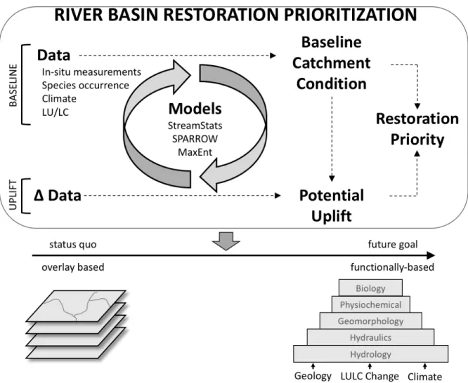
proxies for these functional categories, the extent of available data and models to assess and project changes in nutrient loads, hydrologic regimes, and ecological health make it possible to change the status-quo for restoration planning (Figure 1.1). Additionally, by moving beyond categorization of problems and assets in a watershed and providing trained managers with the raw data specifically related to each function, this framework begins to approach the long-desired need for an underlying scientific understanding of catchment function in restoration planning (Wohl et al. 2005; Beechie et al. 2010).
As the North Carolina regulations require agencies to “develop basinwide plans for wetlands and riparian area restoration with the goal of protecting and enhancing water quality, flood prevention, fisheries, wildlife habitat, and recreational opportunities” (North Carolina General Statute 143-214.10), a new prioritization system was built to systematically provide objective, ecosystem function-based assessment of catchment condition rather than relying solely on a GIS-based overlay and weighting analysis. Here we present the River Basin Restoration Prioritization (RBRP) tool which was developed in conjunction with the North Carolina Department of Environmental Quality (DEQ, formerly Department of Environment and Natural Resources). The RBRP was designed with four primary goals:
1) Distribute scalable data from catchment to river basin scale, 2) Make use of readily available, uniform, and vetted models,
3) Minimize subjectivity and weighting by removing categorical weighting schemes,
Here we focus primarily on the datasets and methods of this tool and present a set of representative results to demonstrate the use as a screening tool for catchment condition and restoration prioritization planning.
1.2. Datasets
One of the overarching goals of this methodology is to make use of readily available, vetted models and datasets. Although distributed, physically-based, or bottom-up, models can provide a small-scale representation of driving processes in a watershed, lumped conceptual and statistically based top-down models provide useful estimates of first-order relationships in catchment condition (Sivapalan et al. 2003). Each of the datasets and models used here are available across North Carolina and as statistical, top-down models can be easily implemented across gauged and ungauged catchments. While bottom-up models may be more appropriate for site-selection, these top-down models offer sufficient coverage and substantially decreased processing time that is key for assessing large volumes of data at a regional scale. The spatial resolution of all input data is equivalent to or finer than the catchment geometry, and can be aggregated to coarser resolutions as needed for scalable analysis. While much of the data refers to in-stream variables, we present input and output data at the catchment scale for visualization and interpretive purposes. All input data sources are presented in Table 1.1.
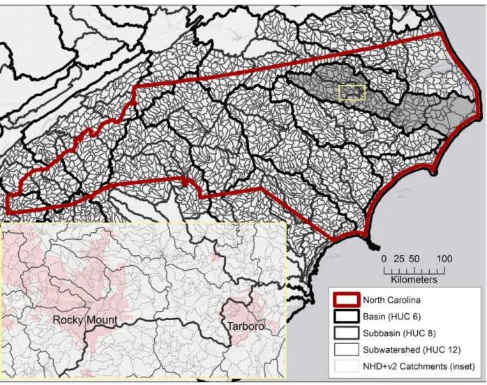
1.2.1 Catchment Geometry and Study Area
1:100,000 blue lines of the National Hydrography Dataset and the 1-arc second National Elevation Dataset. The NHD+v2 flowlines and catchments have a 1:1 association via a common ID, allowing data to be represented at either level. The NHD+v2 is also distributed with numerous associated datasets that provide information regarding local catchment attributes, upslope accumulated attributes, and in-stream data (flow, temperature, etc.) (Moore and Dewald 2016). The NHD+v2 is nested within the Watershed Boundary Dataset (WBD) which allows for spatial aggregation to the multi-level Hydrologic Units (https://nhd.usgs.gov/wbd.html). For the purpose of this tool, we make use of the terminology from both the NHD+v2 and the WBD – catchments refer to the local drainage area for each NHD+v2 stream reach and not the entire upslope area; and the Hydrologic Unit Code (HUC) naming conventions are used to refer to river basins (HUC 6), subbasins (HUC 8), and subwatersheds (HUC 12).
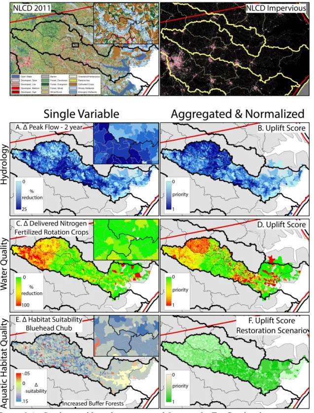
In the context of the NHD+v2 and the WBD, North Carolina encompasses approximately 70,000 catchments, 1,775 subwatersheds, 57 subbasins, and 14 river basins (Figure 1.2). These catchments span four Level III EPA Ecoregions within the state with varying drainage and land cover characteristics, ranging from well-drained coastal plains to the Appalachian Mountains. Elevations range from sea level to greater than 2,000 meters in the western portion of the state. The data presented here focuses on the Tar-Pamlico River basin (HUC 6: 030201). This region falls in the central and eastern portions of the state, north of the Research Triangle, and spans parts of the Piedmont and Coastal Plain ecoregions.
1.2.2 Water Quality
phosphorus) in each NHD+ catchment. Most watersheds lack the water quality monitoring data required to estimate loads, therefore estimates for unmonitored watersheds must be extrapolated. The estimates of stream nitrogen and phosphorus load produced from the SPARROW nutrient models for the southeast region (Hoos et al. 2013) are well suited for analysis of restoration potential. Mean annual load to stream from catchment for the period 1995-2004, centered to 2002, is estimated for each of 392,000 catchments in a 1:100,000 network of streams. The model estimate for each NHDPlus catchment is computed from a statistically derived equation that relates observed nutrient load in streams (from a set of about 300 monitored watersheds) with upstream factors such as fertilizer inputs, area of developed land, permitted wastewater discharges, soil erodibility and thickness, and precipitation. The equation accounts for differential rates among watersheds and streams of terrestrial and stream transport of nutrients. Using a single statistical equation to estimate loads for all watersheds in North Carolina provides a consistent set of estimates with quantified limits of confidence.
The following description of the SPARROW model regression equation is taken from Schwarz et al. (2006), Eq. 1.27, modified by Hoos and McMahon (2009). The load originating within the catchment for reach i (Lcatchmenti) is determined by:
𝐿𝑐𝑎𝑡𝑐ℎ𝑚𝑒𝑛𝑡) = 𝑆,,)𝛼,𝐷, 𝑍)1; 𝜃
1 𝐴 𝑍)5, 𝑍)6; 𝜃5, 𝜃6 78
)9: ,
where
n, Ns = source index where Ns is the total number of individual sources;
n
S = vector of source variables (for example, a measurement of mass placed in the watershed, or the area of a particular land cover); and
n
(across all catchments in the model area) fraction of nutrient input that completes the overland and subsurface phase of transport (i.e. terrestrial transport) to the stream channel.
( )
×n
D = the delivery variation factor, defining the variation among catchments in nutrient landscape attenuation processes. The delivery variation factor is modeled as a series of exponential functions of physical landscape characteristics that influence nitrogen attenuation. The factor for catchment i is multiplied by an to calculate the fraction of input from source n that completes terrestrial transport to the edge of the stream channel in catchment i.
D
Z
= vector of physical landscape variables (for example measured landform or soil characteristics); andD
q
= vector of coefficients, estimated by the model, for the physical landscapevariables.
( )
×A = the stream delivery function, representing the result of attenuation processes acting on load as it travels along the stream channel. Modeled as first-order decay, the stream delivery function defines the fraction of load originating in and delivered to reach i that is transported to the reach’s downstream node.
S
Z
andZ
R= vectors of measured stream and reservoir variables, respectively (examples include stream-water depth or velocity and reservoir areal hydraulic loading); andS
q and qR = vectors of coefficients, estimated by the model, for the stream and reservoir
Conceptually the load or mass of nutrient transported in a stream varies continuously along the segment of stream within a catchment, as mass is added from terrestrial transport pathways distributed throughout the catchment and as mass is assimilated or stored within the channel. The SPARROW model equation parameterizes rates of terrestrial and stream transport and therefore the model tracks mass at the interface between catchment and stream segment (‘edge of channel’ interface) and through the segment of stream channel to the downstream node of the catchment. More commonly (and by default settings) the model estimate of catchment load (incremental or accumulated) is the simulated load at the downstream node of the catchment. For application to restoration potential analysis – where evaluation of watershed condition (sources and terrestrial transport) independent of channel processing is desired – model simulations instead report load at the edge of the channel interface. The set of load estimates produced with this alternate setting is referred to in this paper as SPECL, or Shift Prediction to Edge-of Channel-Load. When nutrient mass flux is referred to henceforth, it is meant to represent this land to water delivery and not necessarily the flux at the outlet of each catchment.
1.2.3 Hydrology
To assess the condition of the hydrologic flow regime in a succinct manner at the catchment scale, the RBRP framework calculates instantaneous peak flows at four return intervals. The USGS StreamStats tools provide a set of equations describing the relationships between landscape characteristics and these peak flows across space, calibrated with streamflow data from gaged basins. Feaster, Gotvald, and Weaver (2014) developed an updated set of regression equations to estimate return period specific flows from upstream watershed characteristics for North and South Carolina which we have adapted and supplemented with additional equations (Mason Jr et al. 2002) to fully represent the hydrologic regime of North Carolina. In order to differentiate hydrologic responses between geographic areas, separate equation sets were developed for each distinct hydrologic region. These regions vary only slightly from the traditional EPA Level III Ecoregions, with some ecoregions being aggregated (Mid Atlantic Coastal Plain and Southeastern Plains) and some Level IV regions included into the dataset as separate areas (Sand Hills). For each catchment, these equations are used to calculate instantaneous peak flows at 2-, 10-, 50-, and 100-year recurrence intervals, allowing the user to assess the response of a catchment and the upslope drainage area to a variety of storm magnitudes.
1.2.4 Habitat Quality
The US Fish and Wildlife Service recently developed a wide-ranging dataset of aquatic indicator species and their probabilistic distributions for the state of North Carolina (Endries 2011). These species occurrence points come from six different sources within the state and have been restructured to match the spatial resolution of the NHD+v2 stream reach and catchment dataset; that is to say that any catchment in which a species was sampled in any of the six datasets will be marked as a species presence location. While an indicator species dataset of this detail is somewhat unique to North Carolina, similar datasets are not uncommon, and national programs like EnviroAtlas (https://www.epa.gov/enviroatlas) are currently providing data layers representing the number of at-risk aquatic animal or plant species for CONUS.
Stream, catchment, and watershed-scale characteristic data is used in conjunction with the species occurrence data to develop the prediction of aquatic habitat quality. These data come in large part from the information served through the NHD+v2 supplemental information. In addition, the RBRP collects data regarding stream temperature, dams, and agricultural production from state level data sources to supplement the information on catchment condition.
1.2.5 Additional Input Data
1.3. Model Description and Methodology
The primary goal of the RBRP workflow is to develop a uniform characterization of the baseline condition for each catchment within the dataset. In order to assess this condition, each subsection of the tool (water quality, hydrology, and habitat quality) is run with the previously described datasets. Because the equation sets and data sources for the water quality and hydrology sections of the model are static and do not require re-runs for new model implementations (i.e. as long as input data remains the same, the same result will be obtained from the models), these baseline values can be calculated for the entire region (North Carolina in this case) or data extent from the outset. Each individual model implementation, however, is meant to be implemented at the HUC 6 scale or finer resolution to match the basin-scale of previous DEQ management tools. Because the spatial distribution and habitat range of indicator species used in the habitat quality subsection is not uniform across space and the importance of each indicator species to local habitat quality varies from region to region, this portion of the model is intended to focus on the extent of the river basin or finer.
landscape elements is required, implementation of these models is meant to be carried out by a trained geospatial analyst and natural resources manager.
1.3.1 Water Quality
The tabular SPARROW output for each catchment in the study area is joined directly to the NHD+v2 catchments. Each catchment then has nitrogen and phosphorus baseline data for a variety of sources, and for both the loading on the catchment as well as the portion that is delivered from the land to water phase. The SPECL data is used as the primary representation of catchment level water quality information. The SPARROW model allows users to view nitrogen and phosphorus data by source and the RBRP workflow retains this source specific data to better inform management decisions. However, in an effort to make output data more concise, multiple agricultural sources are aggregated into a single agricultural loading value. For the nitrogen model, this includes fertilizer from rotation crops, fertilizer from other crops, and nitrogen from manure. For the phosphorus model, this aggregate value includes phosphorus from cultivated crops and phosphorus from pasture/hay. Non-manageable sources of each nutrients (e.g. bedrock sources of phosphorus) are dropped from the model to simplify analysis as well. Therefore, baseline water quality condition is calculated from agricultural, urban, and depositional sources of nitrogen and agricultural and urban sources of phosphorus.
in landscape variables other than source reduction. The results of this potential uplift analysis can therefore be interpreted as either, allowing managers to release priorities that maintain the practitioner’s ability to specify which methods will be used to control or reduce water quality issues.
1.3.2 Hydrology
The peak flow regression equations rely on a finite set of variables, making it relatively simple to calculate the flows across multiple return intervals for each catchment (Table 1.2). As many catchments have portions of their upslope drainage area in multiple hydroregions, an area-weighted mean of the values for each individual hydroregion is used. Accounting for this, the 2-, 10-, 50-, and 100-year instantaneous peak flows are computed for every catchment. Peak flows, when normalized to a depth per unit time or volume per unit area, are typically highest for small catchments and are reduced as drainage area increase. Because the focus is on instantaneous peak flows, the targeted areas are often shifted to the headwaters where management practices can be implemented to reduce runoff and impact these flows. Flood mitigation along trunk streams is not considered to the same degree here but could be included in future versions by considering floodplain extents or levee implementation.
of these areas but could represent an alteration to the landscape which reduces effective impervious surface (e.g. green infrastructure, increased buffer, or run-on infiltration).
1.3.3 Habitat Quality
The habitat function utilizes the Maximum Entropy (Maxent) modeling framework to build species distribution models for key aquatic quality indicator species. Generally, Maxent uses incomplete information on species distribution to predict a probability distribution of maximum entropy (Phillips, Anderson, and Schapire 2006). Maxent offers many advantages in that it requires only presence data along with environmental information for the study area, it can utilize both continuous and categorical variables, and the solutions have concise mathematical definitions which are simpler to analyze.
For each model implementation within a HUC 6, the RBRP user selects a set of key aquatic quality indicator species and calculates species distribution likelihood models for each based on the habitat condition in the catchments in which the species has been noted as present. These individual models are then averaged to represent the aggregate habitat condition in that catchment. It is important for the viability and parsimony of the habitat quality model that an appropriate subset of species be chosen to accurately represent the catchments in the study area. Therefore, the user should be familiar with their study area and the key aquatic indicator species therein.
urbanization/conversion, wetland restoration, and stream restoration. Each of these scenarios alters a set of catchment parameters by some user-defined amount and proceeds to recompute the habitat suitability models for each species in the study area analysis. For example, upstream and downstream distances to dams are calculated to determine a metric of aquatic habitat connectivity. In order to calculate potential uplift in each of these scenarios, the distance to dams is increased by a uniform scalar, and the Maxent distribution models are rerun to determine the effect this change in aquatic connectivity has on species distribution. This change from the baseline species distribution is then considered to be a simple metric of potential habitat quality uplift under the aquatic connectivity aggregate scenario.
1.3.4 Data Aggregation and Visualization
With the goal of avoiding an over-use of subjective weightings in the aggregation and interpretation of model output, raw data for each of the three RBRP submodels is presented for each catchment across the study area. When combining individual output variables (e.g. each return interval for instantaneous peak flows) to create a single submodel score (e.g. hydrology), the influence of each output is, by default, considered equally and a simple arithmetic mean is calculated. However, some variety of data normalization and scoring is required to compare across basins and model implementations. In order to do this, the RBRP implements a max-min normalization of data from each submodel output relative to other catchments in the same subbasin (HUC 8); that is, each catchment within a subbasin is attributed with a 0.0 – 1.0 score for each water quality, hydrology, and habitat quality metric based on the maximum and minimum values for the same variable of the other catchments in that basin.
where zi,j represents the maximum-minimum normalized score for catchment i and measurement
j, and xj represents the raw score for measurement j within the digit HUC of interest. The 8-digit HUC was chosen as it is considered the management unit by NC DEQ. The metrics within each submodel are then aggregated through the following equations:
𝐻𝑦𝑑𝑟𝑜𝑙𝑜𝑔𝑦) =
1
𝑛 (𝑧),<)
,
<9:
𝑊𝑎𝑡𝑒𝑟𝑄𝑢𝑎𝑙𝑖𝑡𝑦) =1 2
1
𝑛 𝑧7)RSTUV, ),<
,
<9:
+ 1
𝑚 𝑧YZT[\ZTS][ ),<
^
<9:
𝐻𝑎𝑏𝑖𝑡𝑎𝑡) = 1
𝑛 (1 − 𝑧),<)
,
<9:
1.4. Results and Illustration of RBRP Use
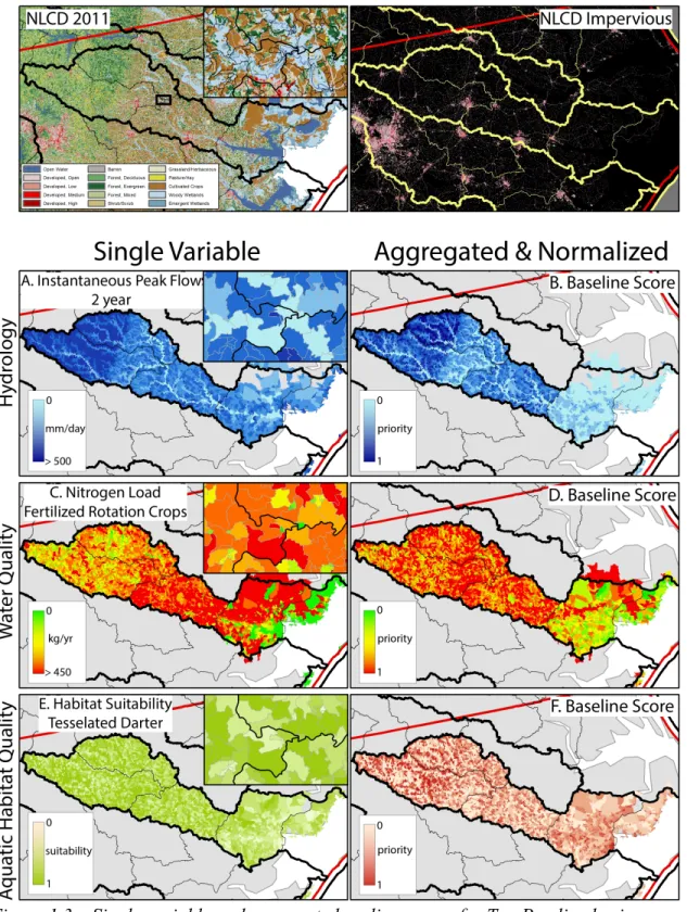
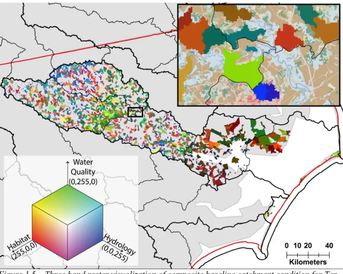
The RBRP provides both raw and relativized scores for each catchment in the study area. Here we present these data for the catchments of the Tar-Pamlico River basin in eastern North Carolina. (HUC6: 030201) and a small subsection near Tarboro, NC, at the confluence of the Tar River and Fishing Creek (Figure 1.3, Figure 1.4). The aggregation and normalization of the baseline and uplift scores is done at the HUC8 level, meaning that each catchment in a HUC8 is relativized based on the range of values in that HUC8; there will be a single minimum and a single maximum value catchment in each river subbasin. We focus here only on the baseline catchment condition data.
1.4.1 Single Variable Output from Submodels
1.4.1.1 Baseline Catchment Condition
impervious surface or developed area. Along with the patterns of drainage area and land use, there is a sharp transition in flow response at the boundary of the Coastal Plain and Piedmont hydrologic regions.
The SPARROW model output provides numerous raw data points for nitrogen and phosphorus loads, one for each nutrient source group in the catchment. The spatial patterns seen in the Tar-Pamlico basin for rotation crop fertilizer-sourced nitrogen are driven largely by the patterns of agricultural land use in the area (Figure 1.3C). Moving from the less cultivated Piedmont to the Coastal Plain, delivered nitrogen loads increase substantially. In the outermost coastal plain, when very low slopes and expansive wetland areas begin to dominate the landscape, delivered nitrogen loads from rotation crops again reach a minimum. In the area around Tarboro, delivered rotation crop nitrogen loads are especially high in catchments where the agricultural land is in close proximity to the flow lines. For the additional nitrogen sources and those sources of phosphorus, the patterns exhibited by land use on both accumulation and removal of nutrients hold in a similar fashion to the rotation crop derived nitrogen.
habitat suitability over a study area with the use of representative aquatic habitat quality indicator species.
1.4.1.2 Potential Uplift
Potential uplift within the hydrology submodel is driven entirely by a reduction in impervious surface. Again, while mathematically this reduction represents a removal of impervious surfaces, the same or similar responses could be obtained by reducing effective impervious areas, which has been shown to be a better predictor of stream conditions than total imperviousness (Walsh, Fletcher, and Ladson 2009). The most effective reductions in 2 year peak flows tend to occur in those areas that have small drainage areas and high levels of impervious surface (Figure 1.4A). The sharp transition between the Coastal Plain and Piedmont regions is not apparent in this case as the metric for potential uplift is based on a change from previous peak flow volumes.
Response to reductions in nitrogen loads from fertilized rotation crops is relatively low across the Tar-Pamlico basin though small hotspots of changes in delivered loads are found in the upslope portions of the Upper Tar subbasin and in the Outer Coastal Plain (Figure 1.4C). Much of the upstream area of the basin, northeast of the Coastal Plain-Piedmont boundary, exhibits a stronger response to changes in nutrient sources. With any of the individual sources of nitrogen or phosphorus, the spatial distribution is not homogenous. Therefore, the potential uplift response for each nutrient source is contingent on the existence of those sources.
(Figure 1.4E). Because the model is probability based, the response of species presence likelihood is not constrained to only increases or decreases but can range from total elimination to doubling or tripling of likelihood in a given catchment. This is seen in part of the area around Tarboro, where many catchments show increases in bluehead chub presence likelihood but others show no change or even a decreasing likelihood.
1.4.2 Submodel Aggregation
1.4.2.1 Function Specific Visualization
As each of the individual model elements are aggregated to a submodel baseline score, the individual influence of each element decreases. The calculation and normalization of baseline scores also accounts for the distribution of values within a single HUC 8. Therefore, while the raw values may be uniformly higher in one subbasin than in another, each subbasin will still have values ranging from 0-1.
The hydrology model baseline score exhibits many of the same patterns as those in the two year recurrence interval (Figure 1.3B). Trunk streams with large drainage areas show relatively little impact from large flow events. Small headwater catchments remain as the key areas to target in order to mitigate high peak flood flows over all recurrence intervals. Within each HUC8, catchments of the lowest priority are uniformly found along the main stems of the Tar River and Fishing Creek while the high priority catchments follow drainage area and land use patterns.
are identified as key areas of focus for reducing the delivery of nitrogen and phosphorus to waterways. In the upstream subbasins, especially in the Upper Tar (HUC 8: 03020101) which encompasses Rocky Mount and much of Tarboro, urban sources of nutrients are also found to be key drivers of the overall water quality condition of the subbasin.
Habitat quality metrics for individual species are calculated as habitat suitability metrics, scaling from poor quality to good quality. As the other submodels scale from good quality to poor quality in a single catchment, the aggregation of multiple species suitability models is inverted to return a metric of habitat quality that also scales from good to bad quality, or low priority to high priority for restoration. The suite of species modeled for the Tar-Pamlico basin show negative response to the limited urban areas within the basin (especially in the Upper Tar subbasin) and some response to conditions along the estuary mouth of the Tar River (Figure 1.3F).
1.4.2.2 Aggregation of Function-Specific Potential Uplift Metrics
As with the baseline submodel aggregation, the aggregated potential uplift metrics help elucidate spatial patterns across the model elements within each subbasin. Where high values of potential uplift are uniform across individual model elements, catchments exhibit a high priority for restoration planning.
reduction may be uniformly higher than in adjacent subbasins, the high priority areas are more localized (Figure 1.4D).
The aquatic connectivity, wetland restoration, and stream restoration habitat quality uplift scenarios all scale from little influence of catchment alteration to high impact, and therefore yield uplift scores that scale from low priority to high priority. The avoided conversion scenario is based on the response of species within a catchment that experiences development. Because of this, the avoided conversion scenario inverts the response of species to the development (typically reduced presence likelihood with increased urbanization) to highlight catchments in which development should be avoided in order to preserve aquatic habitat quality. In the Tar-Pamlico basin, the stream restoration suite of uplift scenarios exhibits high priority areas for all species in small headwater catchments within the upstream subbasins and relatively high priority across all catchments in the outer Coastal Plain (Figure 1.4F).
1.4.2.3 Integrated Function Visualization
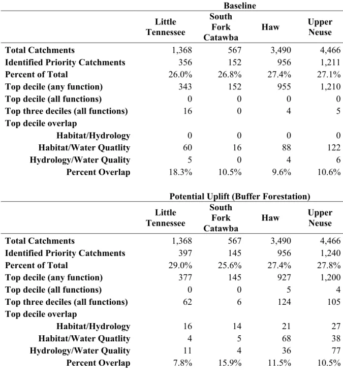
study area. This 10%/30% data filter does not necessarily represent a functional split in the data, but provides users with a framework to visualize a subset of data representing likely problem areas. These values can be changed to visualize more or fewer catchments for potential further action. The region surrounding Rocky Mount stands out for its detrimental impacts on both water quality and habitat quality, while the upper portions of the Fishing Creek subbasin exhibit poor quality scores for both hydrology and habitat quality. By analyzing the normalized and aggregated data from all submodels in this manner, unique color combinations emerge that indicate the influence of different watershed functions on the condition of the catchment, and watershed planners can work towards targeting spatially contiguous areas where restoration efforts may have the most impact.
1.5. Discussion
improvements can be made that can improve the success and provide more specific metrics of outcomes of the individual projects.
In carrying both raw data and aggregated and normalized scores through the prioritization process, the RBRP provides users with a simple visualization tool which represents an aggregation of big data while also directly tying the outcomes to vetted models with strong ecological backing. The normalized scores utilized to calculate final catchment condition scores are presented with minimal subjective weighting in an effort to focus on the impact of individual model elements and not that of the element weights themselves.
1.5.1 RBRP and Previous Prioritization Systems
the tools. First, as the focus of the basin’s previous TLW delineation was water quality condition, many of the catchments outside of the TLW boundaries are those highlighted for their hydrologic and habitat quality condition. Additionally, the former RBRP workflow allowed planners to add or remove watersheds from the TLW list based on a variety of factors, including local input. Those catchments identified as priorities for restoration in the new workflow are highlighted specifically because of the underlying data supporting the catchment condition.
1.5.2 Data Updates and Model Extensibility
planners and policymakers can work to update this work in a way that can additionally benefit restoration prioritization tools.
We are now working in a landscape in which increasingly finer resolution data over greater spatial scales is becoming available and can be incorporated into this type of framework. Because of this, many opportunities exist to supplement or improve those data sources already used in the RBRP. The water quality and hydrology models are both predicated on models developed for the eastern or southeastern United States. Both of these models, with appropriate expertise and data availability, could be redeveloped with data focused solely in North Carolina or within the immediate drainage area. This would allow for improved predictions of peak flows and nutrient loading specific to the state. The habitat model could be supplemented in a variety of ways, either by adding and refining key aquatic indicator species or by improving the catchment condition datasets that are used to build the Maxent species distribution models. A primary need to improve aquatic suitability assessment is in stream information, characterizing bed material and channel morphology. Current efforts to develop bed material estimates at the NHD+ reach scale by the USGS and others are underway and could be easily incorporated into this analysis (Gomez-Velez and Harvey 2014; Wang et al. 2013).
1.6. Concluding Remarks
Table 1.1 – Input data sources for catchment baseline characterization
Input data sources for RBRP baseline characterization workflow.
Function/Usage Data Source
Catchments 1:100,000 scale NHD+v2 Catchments USGS & Horizon Systems Corp.
Water Quality Nitrogen Atmospheric Deposition
USGS Eastern US SPARROW Agricultural
Urban
Phosphorus Agricultural Urban
Hydrology Impervious Surface NLCD 2011 24-hour, 50-year Maximum Precipitation NOAA Atlas 14, Volume 2
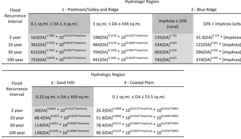
Table 1.2 – Regional instantaneous peak flow equations for 2-, 10-, 50-, and 100-year recurrence intervals
Hydrology submodel regional instantaneous peak flow equations for 2-, 10-, 50-, and 100-year recurrence intervals. DA: drainage area, ImpArea: percent upslope impervious, DevArea: percent upslope developed (NLCD class 21-24). Equation set developed from Feaster, Gotvald, and Weaver (2014) and Mason Jr et al. (2002).
Flood Recurrence
Interval
Hydrologic Region
1 - Piedmont/Valley and Ridge 2 - Blue Ridge
0.1 sq.mi. ≤ DA ≤ 3 sq.mi. 3 sq.mi. ≤ DA ≤ 436 sq.mi. ImpArea ≤ 10% (rural) 10% < ImpArea (urban)
2 year 163(DA)0.7089 * 10(0.0133*ImpArea) 198(DA)0.5735 * 10(0.0101*ImpArea) 135(DA)0.702 33.3(DA)0.739 * (ImpArea)0.686 10 year 381(DA)0.7536 * 10(0.0076*ImpArea) 484(DA)0.5539 * 10(0.0060*ImpArea) 334(DA)0.662 122(DA)0.655 * (ImpArea)0.515 50 year 632(DA)0.7903 * 10(0.0037*ImpArea) 794(DA)0.5428 * 10(0.0037*ImpArea) 602(DA)0.635 296(DA)0.602 * (ImpArea)0.396 100 year 753(DA)0.8038 * 10(0.0024*ImpArea) 941(DA)0.5386 * 10(0.0028*ImpArea) 745(DA)0.625 374(DA)0.593 * (ImpArea)0.358
Flood Recurrence
Interval
Hydrologic Region
3 - Sand Hills 4 - Coastal Plain
0.22 sq.mi. ≤ DA ≤ 459 sq.mi. 0.1 sq.mi. ≤ DA ≤ 53.5 sq.mi.
Figure 1.1 – River Basin Restoration Prioritization workflow
Figure 1.2 – North Carolina’s hydrographic geography
Figure 1.3 – Single variable and aggregate baseline scores for Tar-Pamlico basin
Figure 1.4 – Single variable and aggregate uplift scores for Tar-Pamlico basin
Figure 1.5 – Three band raster visualization of composite baseline catchment condition for Tar-Pamlico basin
Figure 1.6 – Comparison of composite baseline score with previous targeted local watersheds
SUMMARY AND TRANSITION
CHAPTER II.
SPATIAL PATTERNS IN FUNCTION-BASED RESTORATION PRIORITIZATION ACROSS NORTH CAROLINA
Abstract
2.1. Introduction
Despite continued efforts to protect waterways from degradation, anthropogenic development, land use change, and a changing climate have caused freshwater quality issues to persist. Nutrient loading of nitrogen and phosphorus from agricultural, urban, and other sources has led to substantial changes in water quality, negatively impacting not only the aquatic habitat quality, but also lowering the economic and aesthetic potential of these areas (Boesch, Brinsfield, and Magnien 2001; Kemp et al. 2005; Vitousek et al. 1997; Carpenter et al. 1998). Increased pressure on the hydrologic regime has also resulted from expanding urban and otherwise developed areas, with changes in infiltration capacity and stormflow generation leading to degradation of headwater streams and altered flooding regimes downstream (Walsh et al. 2005).
function-based approach has also emerged to define a hierarchy of interrelated processes influencing the condition of the watershed (Harman et al. 2012).
This turn towards a function-based restoration design has allowed for the movement away from form-based or structural design (Bronner et al. 2013; Palmer, Hondula, and Koch 2014). By defining key watershed parameters and their role in the baseline catchment condition, workflows and models can be developed not only to design and monitor specific projects but also to help screen and prioritize catchments for restoration across a broad region. With this in mind, widely distributed, vetted data sources and models can be manipulated to represent individual parts of the functional pyramid defined by Harman et al. (2012), one that describes the interconnected, hierarchical structure of watershed functions and their influence on ecosystem health.
water quality. The RBRP was designed as part of an effort to account for this spatial variability and to present equally valuable data across these gradients.
2.2. Methods
2.2.1 Study Area
clipped at the state boundary. This state boundary clipping does not affect any of the other study basins1.
2.2.2 Study Methods
Following the RBRP workflow laid out in the previous chapter, we characterized the baseline and potential uplift conditions related to hydrology, water quality, and aquatic habitat quality for every catchment within each of four basins. Briefly, the hydrologic condition of each catchment was assessed using the instantaneous peak flow regression equations for 2-, 10-, 50-, and 100-year recurrence intervals (Feaster, Gotvald, and Weaver 2014; Mason Jr et al. 2002). Water quality condition was assessed using nitrogen and phosphorus data from the USGS SPARROW model (Hoos et al. 2013). Nitrogen baseline condition was calculated with the SPARROW Shift Prediction to Edge-of-Channel Load (SPECL) model version for urban areas, atmospheric deposition, and an aggregated value for all agricultural sources which specifically accounts for nutrient flux to the edge of the channel and removes effects of in stream processes in order to better match the unit of management for restoration. Phosphorus baseline conditions were calculated using the same SPECL loads for urban and aggregated agricultural sources. The aquatic habitat quality was assessed by predicting modeled species distributions based on landscape attributes via MAXENT (Phillips, Anderson, and Schapire 2006). Five key aquatic indicator species’ distributions (as selected for each hydrologic region by NC DMS planners) were modeled to create an aggregate measure of aquatic habitat quality (Endries 2011).
and recomputing the altered conditions. That is, reduction of impervious surface or reduction in nitrogen or phosphorus sources are used as a proxy for effective treatment in the hydrology and water quality models, respectively. These changes represent a wide range of management practices that may manifest in similar effects on watershed health, without prescribing a specific management practice. The percent change in catchment condition relative to the baseline was used as the metric for a catchment’s uplift potential. For the aquatic habitat quality submodel, the buffer forestation scenario was run to calculate each species’ modeled response to increases in streamside buffer forest. Increased species presence likelihood indicates higher uplift potential.
Data were visualized and areas highlighted for restoration prioritization using a three band raster visualization in which each of the RBRP submodels was attributed to a red, green, or blue raster band and visualized as a composite image. Without additional input from local watershed managers and as to not bias results towards any one submodel input, the default even weights and arithmetic means were used for aggregation of each submodel variable to the function score. We note that these weights can be adjusted by the software user based on local conditions and priorities.
2.3. Results
2.3.1 Baseline Conditions
colored (Figure 2.2). In theory, a catchment that has the worst baseline condition in all three submodels will be seen as white in these composite images, although this is not seen in practice in these study regions. Again, the 10% and 30% filter thresholds are used to visualize a subset of the data and allow managers to analyze contiguity of potential problem areas; these values are determined a priori and can be changed by the user to visualize more or fewer catchments.
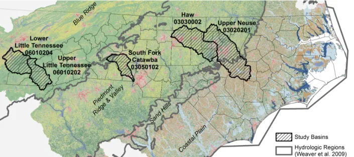
The baseline condition workflow identified 26%-28% of the catchments in each of the four basins as potential priority areas for restoration (Table 2.1). In the Little Tennessee subbasins 16 catchments, or 4.5% of the total, were in the top three deciles for all three functions while no catchments were in the top decile across all three functions. For the top decile condition across any single function, 343 catchments were identified, with 60 catchments in this worst baseline condition group for both aquatic habitat and water quality. In the remaining three subbasins, few catchments satisfied the top three deciles condition, with zero, four, and five catchments identified in the South Fork Catawba, Haw, and Upper Neuse respectively. Similar to the Little Tennessee subbasin, the most common overlap of worst decile condition is between aquatic habitat and water quality condition in the other three basins. In the Little Tennessee, 18% of the catchments are identified as being in the worst decile of baseline condition for more than one of the functions, while the other three basins only have around 10% overlap between functions.
2.3.2 Potential Uplift Scenario
where current conditions are the worst, but where altering driving variables in each submodel manifests in large changes in catchment condition.
The potential uplift analysis incorporating the buffer forestation scenario in the aquatic habitat model identified 25%-29% of the catchments in each basin as candidates for management (Table 2.1). Catchments primarily fulfilled the top decile in any function condition, but a larger portion of catchments fell into the top three deciles for all three conditions than during the baseline analysis. Additionally, four and five catchments in the Haw and Upper Neuse subbasins respectively were in the highest potential uplift decile across all three conditions, indicating areas that may be especially responsive to management actions. The potential uplift workflow also identified a more consistent co-occurrence of overlap between functions identified for prioritization in each catchment. In each subbasin, between 7%-16% of the catchments were identified as priority areas in more than one function.
2.4. Discussion
2.4.1 Interpreting Baseline and Potential Uplift Prioritization Patterns
Poor hydrologic condition is commonly found in urbanized and developed areas across all regions, and especially in catchments with no upstream neighbors. The transition between hydrologic regions, as seen in the Upper Neuse and South Fork Catawba subbasins, also influences this hydrologic response to a certain degree as the peak flow regression equations shift across region boundaries. For example, while there are some small developed regions in the southeast of the Upper Neuse, the flood peak response in the coastal plain is much lower and the hydrologic baseline condition of these catchments is therefore relatively better than comparable catchments around the Raleigh and Durham metropolitan areas in the northwest of that basin. In the Little Tennessee, because the peak flow equations predict very little flood response in the forested catchments that make up a large portion of this basin, catchments with any appreciable urbanization exhibit much higher peak flow response relative to their neighbors and stand out when using the raster visualization method. Additionally, as data are presented as depth per unit time or volume per unit area, the highest peak flows are typically found in smaller headwater catchments where urban area covers larger proportions of the drainage area. While to some degree this decision downgrades management practices that mitigate flooding along trunk streams, the focus on headwater reaches promotes localized practices that can reduce flashy runoff, the effects of which will also benefit downstream areas.
quality baseline condition, as can be seen by the location of catchments visualized in the green band (Figure 2.2). Alternatively, the southeastern portion of the Upper Neuse and southern half of the South Fork Catawba subbasins are highlighted as the primary contributors of poor catchment water quality conditions because of the dominance of row crop agriculture.
As the aquatic habitat baseline conditions are derived from an aggregate of five species with differing responses to landscape variables, the spatial patterns in this function are not as readily tied to land cover as in the hydrology and water quality submodels. However, percent contribution of variables to each species’ distribution model offers insight to driving factors of poor aquatic habitat quality. Within the Little Tennessee, stream temperature arises as a key contributor across all five species, with distance to dams also affecting species distribution models.
In the remaining three subbasins, aquatic habitat quality was commonly driven by a metric of stream size, whether that was total drainage area, stream order, discharge or velocity. Presence or absence of forested areas and developed areas in the catchments was also a uniformly high contributor to each species’ distribution model. Even with the different sets of modeled species, the relatively similar land use patterns in these basins largely drove species presence predictions and aquatic habitat quality models.
northern headwaters near Hickory and to the south near Lincolnton and Gastonia. There is a contiguous region of high potential uplift for water quality in the northwestern headwaters of the catchment, an area downstream of the relatively pristine South Mountains State Park but with some interspersed agriculture. The Haw and Upper Neuse again show higher potential uplift in conjunction with developed areas, in this case indicating areas of higher source problems with a greater potential for reduction. Areas of high potential uplift for aquatic habitat quality tend to be more isolated in these two basins. As the aquatic habitat potential uplift in these scenarios is based on response to increased buffer forests, these areas highlight stream reaches in which buffer forestation is both possible and has high positive impact on species presence likelihood.
The Tar-Pamlico basin exhibits many of the same baseline and potential uplift metrics as the Haw and Upper Neuse subbasins, as shown in Chapter 1, Section 4 and Figures 1.3-1.5. Large, contiguous areas of poor baseline condition are concentrated around the small urban area of Tarboro, and many of the catchments identified for poor baseline condition in the hydrology submodel fall in the headwaters of the basin, in the Piedmont rather than the Coastal Plain. The same transitions in hydrology and water quality response across the ecoregion boundary take place in this basin as well.
2.4.2 Tracing root causes of impairment
Within the Haw and Upper Neuse river basins, we can examine an underlying variable of each of the submodels to help interpret the baseline aggregate data (Figure 2.4). Urban areas in the western portion of the Haw and along the joined border of the two basins exhibit poor baseline quality for both the two year peak flow and incremental nitrogen loads. These patterns clearly stand out in the aggregate baseline data with the same areas being highlighted as potential candidates for restoration. High incremental nitrogen loads and low presence likelihoods for a single species (N. leptocephalus) in the southeastern, downstream portion of the Upper Neuse come together to highlight areas of potential restoration interest with these functions in mind.
The same analysis of data from each individual model element can be very useful when examining a single catchment. For one catchment near the Duke University campus that is highlighted through the baseline catchment condition analysis, we can trace back through the data to help elucidate possible driving factors of impairment (Table 2.2). When compared against other catchments in the Haw River subbasin, this catchment ranks in the worst modeled 27% for hydrologic condition, 15% for water quality, and 20% for aquatic habitat quality. Being able to note that urban sources of nutrients are a potential driver of catchment condition and that the catchment conditions are especially poor for some but not all fish species can help direct planners in how they may move forward with restoration planning in this area. Although this catchment is not in the top 10% in any one function, poor baseline condition across all three functions may influence how restoration dollars are spent in this area.
compared at a scale that maintains hydrologic connectivity and differs from arbitrary political units.
2.4.3 Understanding data and model effects on output
The effects of these underlying model elements are not unique to any one basin or submodel. Other interesting data artifacts are also found in the response of the water quality model in the South Fork Catawba subbasin (Figure 2.5C). The uppermost headwaters of the subbasin drain the South Mountain State Park, a wilderness area with little to no development impact (>98% canopy, <1% developed). However, parts of this region exhibit high modeled delivery ratios for nutrients relative to their downstream neighbor. This phenomenon is attributable to the landscape position and topography of these upstream catchments. While many of them contain no agriculture, those that are cultivated are at risk for high nutrient delivery because of the steeper slopes, soil properties, and proximity of cultivatable land to streams. The downstream portions of the subbasin, while containing more agriculture, contribute less of their total applied nutrient load to the stream than these upstream catchments. These patterns manifest themselves clearly in the potential uplift output for this subbasin as well, with high potential water quality uplift noted in the same region (Figure 2.3).
2.4.3 Caveats with the NHD+v2 catchment dataset
detailed description of how the NHD was developed, including the flow-line digitization from the USGS 1:100,000 topographic quads, but do not mention that the drainage density and catchment size could vary substantially between quads (Figure 2.7). Although this difference across quad boundaries is visibly notable, there exist few options for correcting the existing data. Because of this, the effect of catchment area on analysis must be kept in mind. Local or state agencies have been tasked with maintaining and stewarding their local NHD data, but the fact that the blue lines for the national scale data were digitized at widely varying resolution remains a cause for concern when attempting to utilize the data across large regions.
2.5. Conclusion
Table 2.1 – Catchments identified as baseline and potential uplift priorities
Baseline and potential uplift analysis results for each of the four river subbasins, including counts of all catchments identified with 10%/30% filter. Approximately 25% of all catchments were identified as potential management areas in each basin. The distribution of catchments in the worst decile in two or more functions varies across basins.
Baseline Little Tennessee South Fork
Catawba Haw
Upper Neuse
Total Catchments 1,368 567 3,490 4,466
Identified Priority Catchments 356 152 956 1,211
Percent of Total 26.0% 26.8% 27.4% 27.1%
Top decile (any function) 343 152 955 1,210
Top decile (all functions) 0 0 0 0
Top three deciles (all functions) 16 0 4 5
Top decile overlap
Habitat/Hydrology 0 0 0 0
Habitat/Water Quatlity 60 16 88 122
Hydrology/Water Quality 5 0 4 6
Percent Overlap 18.3% 10.5% 9.6% 10.6%
Potential Uplift (Buffer Forestation)
Little Tennessee South Fork Catawba
Haw Upper
Neuse
Total Catchments 1,368 567 3,490 4,466
Identified Priority Catchments 397 145 956 1,240
Percent of Total 29.0% 25.6% 27.4% 27.8%
Top decile (any function) 377 145 927 1,200
Top decile (all functions) 0 0 5 4
Top three deciles (all functions) 62 6 124 105
Top decile overlap
Habitat/Hydrology 16 14 21 27
Habitat/Water Quatlity 4 5 68 38
Hydrology/Water Quality 11 4 36 77
Table 2.2 – Composite baseline data for single NHD+v2 catchment
Selected baseline data for a single NHD+v2 catchment (COMID: 8893134), located on the Duke University campus in the Haw River subbasin. This catchment ranks within the top 30% in all three functions and is a potential candidate for restorative action based on the baseline condition. The rank value is relative to the other catchments with the same 8-digit HUC (03030002). It must be noted that the peak discharge values are instantaneous peaks. The two year peak flow converts to approximately 772 cfs. A USGS stream gage just downstream of the outlet of this catchment (USGS 0209722970) reports a peak discharge over its period of record (2009-2017) of 1,010 cfs.
Single Catchment Model Output
ComID 8893134
HUC 12 030300020601
Area (sq. km.) 1.786
Total Drainage Area (sq. km.) 5.295
Nitrogen - Atmospheric 1.94
kg/ha/yr Nitrogen - Urban 5.72
Nitrogen - Agriculture 0.23
Phosphorus - Urban 0.64 kg/ha/yr Phosphorus - Agriculture 0.07
Aphredoderus sayanus 0.019
occurrence likelihood
Etheostoma flabellare 0.056
Moxostoma collapsum 0.047
Nocomis leptocephalus 0.213
Noturus insignis 0.180
Peak Discharge - 2 yr 357.2 mm/day (instantaneous
peak) Peak Discharge - 10 yr 564.7
Peak Discharge - 50 yr 719.8 Peak Discharge - 100 yr 786.3
Hydrology Rank 954
of 3,490 catchments Water Quality Rank 534
Figure 2.1 – Four study basins for River Basin Restoration Prioritization assessment
Figure 2.2 – Composite baseline score for four study basins
Figure 2.3 – Composite uplift score for four study basins
Figure 2.4 – Composite baseline score and single input variable from each submodel to trace model input influence
Figure 2.5 – Analysis of influence of data and model structure on prioritization output
Figure 2.6 – Variation of catchment size across USGS 1:100k topographic quad boundaries
Figure 2.7 – Boxplots of catchment area by USGS 1:100k topographic quads
CONCLUSIONS
In this thesis, we have demonstrated the use of a novel restoration prioritization toolkit that makes use of readily available data sources. This tool provides a new framework through which planners and managers across the country can reconfigure how catchments are prioritized for the use of restoration dollars. The incorporation of the regional regression equations, SPARROW model, and species occurrence dataset into the RBRP offers a novel use for these widely-distributed data to benefit watershed planning. Additionally, the structure of the workflow to prioritize catchments relative to their subbasin while still distributing non-normalized baseline and uplift conditions affords watershed planners the opportunity to not bias restoration solicitations in one subbasin over another but to still understand the baseline conditions and potential impact of these projects. In testing model output in four diverse subbasins across North Carolina, we found that the model performs well in heterogeneous basins. The relative influence of urban and agricultural areas on model output remains high across the state, partially because of the structure of the input data sources, but also because these areas are key drivers of watershed condition. As expected, overall current catchment condition generally improves in the Blue Ridge relative to the rest of the state, but sensitivity is high. The RBRP structure maintains the ability to highlight areas of interest for potential restoration even in comparatively healthy basins.
prioritization workflows that better characterize single functions, but we believe the representation of general ecosystem function presented here provides a unique and eminently useful tool to further regional analysis of restoration prioritization. While validation of the priorities identified through this workflow is difficult as no similar priorities existed previously, the use of the datasets and methodology employed here provides a substantive framework for monitoring and follow-up after project implementation in prioritized areas.