THREE TESTS OF DIMENSIONALITY IN STRUCTURAL EQUATION MODELING: A MONTE CARLO SIMULATION STUDY
Niantao Jiang
A thesis submitted to the faculty of the University of North Carolina at Chapel Hill in partial fulfillment of the requirements for the degree of Master of Arts in the Department of
Sociology.
Chapel Hill 2006
ABSTRACT
Niantao Jiang: Three Tests of Dimensionality in Structural Equation Modeling: A Monty Carlo Simulation Study
(Under the direction of Kenneth Bollen)
The issue of dimensionality is essential to social science research but few researchers have
empirically tested the dimensionality of theoretical constructs. One main reason is the
uncertainty of how best to proceed. With the development of structural equation modeling
with latent variables, several tests are available for researchers to choose. In this study,
drawing on statistical theory and prior researches, I empirically assess the performance of
likelihood ration test, confidence interval test, and vanishing tetrads test using data generated
from Monte Carlo simulations.
The study results show the likelihood ratio test did reasonably well. It does not show
obvious signs of impact of the violation of boundary condition when testing for
dimensionality. While overall the confidence interval test method appears to be too
conservative, the vanishing tetrads tests for dimensionality works best for models with few
TABLE OF CONTENTS
Page
LIST OF TABLES... iv
LIST OF FIGURES... v
Section 1. INTRODUCTION... 1
2. LIKELIHOOD RATIO TEST... 4
3. CONFIDENCE INTERVAL TEST... 8
4. VANISHING TETRADS TEST... 8
4.1 Basic Concepts... 8
4.2 Test Steps... 11
4.3 Test Properties... 15
5. SIMULATION DESIGN... 15
6. SIMULATION RESULTS... 20
6.1 Confidence Interval Test... 20
6.2 P-Value of LRT/VTT for Nested Model... 22
6.3 Distribution of Chi Square Difference... 24
7. DISCUSSION AND CONCLUSION... 29
7.1 Main Findings... 29
7.2 Limitations and Future Research... 31
LIST OF TABLES
Table Page
1. Experimental Design Conditions... 18
2. Results of 95% Confidence Interval Test... 21
3. Number of P-Value below 0.05 significant level for Nested Test.………... 23
4. Tests Results for whether Likelihood Ratio Test Statistics for
Nested Models Follow a 1 d.f. Chi-Square Distribution..………... 26
5. Tests Results for whether Vanishing Tetrads Test Statistics for
LIST OF FIGURES
Figure Page
1. INTRODUCTION
An often asked question in sociology and other social science disciplines is whether a
theoretical construct is unidimensional or multidimensional. Researchers have done various
studies on the dimensionality of important theoretical constructs like alienation (Seeman,
1959; Kohn, 1976), bureaucracy structure (Blau, 1967; Child, 1972; Hall, 1963; Pugh et al.,
1968; Reimann, 1973; Samuel and Mannheim, 1970), political democracy (Bollen, 1979;
Bollen 1980; Cutright, 1963; Jackman, 1975), and social capital (Bourdieu, 1983; Coleman,
1988; Lin, 2001; Narayan and Cassidy, 2001; Paxton, 1999; Portes, 1998; Putman, 2001).
Such questions are essential to social science research because misspecification of the
dimensions can lead to incorrect empirical results. On the one hand, if a construct is
unidimensional, using several measures as separate independent variables would most likely
cause severe multicollinearity problem (Blalock, 1963). On the other hand, if a construct is
multidimensional and a single measurement is employed, we would probably only catch one
dimension of the construct, which inevitably would cause trouble in discovering what really
is going on with the construct and its related variables. As Bollen and Grandjean (1981) put it,
“The dimensionality question is crucial to the integration of theory and research, because it draws attention to the implicit theoretical assertions in any operational definition, and
therefore emphasizes the need to incorporate explicit measurement models in causal models.”
However, there have been few sociological examples where dimensionality is empirically
explored during the past several decades. Part of the reason might be that most researchers
need to test whether the correlation between two latent variables is one. This follows since if
two dimensions are really a single dimension, then the two dimensions should be perfectly
correlated when treated separately. With the development and increasing interest of advanced
statistical techniques in the social science, especially structural equation modeling (SEM)
with latent variables, several tests are available for researchers to choose.
Structural equation modeling is a very general and powerful multivariate analysis
technique that includes specialized versions of a number of other analysis methods as special
cases. Causal modeling, factor analysis, path analysis, regression models, covariance
structure models, and correlation structure models all could be seen as special cases of SEM.
A structural equation model implies a structure of the covariance matrix of the observed
variables in an analysis. Once the model’s parameters have been estimated, the resulting
model-implied covariance matrix can then be compared to the sample covariance matrix. If
the two matrices are consistent with one another, then the structural equation model can be
considered a plausible explanation for relations between the measures. Thus SEM is a largely
confirmatory, rather than exploratory, technique. That is, a researcher is more likely to use
SEM to determine whether a certain model is plausible, rather than using SEM to perform an
exploratory search for a suitable model--although SEM analyses sometimes involve a certain
exploratory element.
In SEM, interest usually focuses on latent constructs—abstract psychological or
sociological variables like “intelligence” or “socioeconomic status”—rather than on the
manifest variables that measure these constructs. With SEM, the reliabilities of each indicator
of the latent variables can be assessed. When predictor variables do not account for changes
between the variables or because of poor reliability of the operational measures of those
variables. SEM assesses the degree of imperfection in the measurement of underlying
constructs and distinguishes between less than perfect measurement of variables and
nonrandom, unexplained variance. By explicitly modeling measurement error, SEM users
seek to derive unbiased estimates for the relations between latent constructs. To this end,
SEM allows multiple measures to be associated with a single latent construct. These features
of SEM have led to increasing interest in it in psychology, sociology, organization behavior,
marketing, education and other disciplines.
Among the many applications of SEM, testing for dimensionality of a construct is a
significant one. There are several methods by which researchers can test whether two latent
variables are perfectly correlated in structural equation modeling and the most commonly
used one is the likelihood ratio test, which is based on maximum likelihood statistical theory.
Several researcher have used this test to examine dimensionality of measures by testing
whether the correlation between two constructs was one or not (Joreskog, 1979; Bollen and
Grandjean, 1981; Parker, 1983). However, when dealing with testing for dimensionality of a
construct, one of the key assumptions of the likelihood ratio test, that the true parameter
value is interior to the parameter space, is violated. As I will detail below, this violation
raises questions about the validity of the likelihood ratio. There are other tests that might be
considered including putting confidence intervals around the estimated correlation with the
standard errors, or applying a vanishing tetrads test of dimensionality.
This master paper examines the LR test and other tests of perfect correlations to determine
which works the best. In addition to reviewing these tests of dimensionality, this study will
sample sizes and several different model specifications. The goal is to evaluate which
dimensionality test(s) is most accurate and provide recommendations about which tests
perform best so as to give practical guidance to researchers interested in testing
dimensionality.
The remaining paper is organized as follows: In the next section, I will review the formal
basis of the likelihood ratio test and explain why the test of perfect correlation falls outside
the classical LR test. Next I will describe the test of dimensionality using confidence
intervals with asymptotic standard errors. Then I will introduce the vanishing tetrads test, its
properties, and the steps to perform the test. The fifth section outlines the design of a Monte
Carlo simulation used to address my research question. The last section reports the
simulation results across the different experiment conditions. I conclude with a comparison
of the performance of the different test methods for testing the dimensionality of a theoretical
construct.
2. LIKELIHOOD RATIO TEST
Among all the tests available to examine whether two latent variables are perfectly
correlated in structural equation modeling, the most commonly used one is the likelihood
ratio test, which is based on maximum likelihood theory.
Assume that the distribution of the random variable Y is given by f(y;θ) where θdenotes a vector of possibly unknown parameters (θ∈Θ). The log-likelihood function corresponding to a random sample of size N is given by
∑
=
iln f(yi; )
)
(θ θ
with the maximum likelihood estimator of θ being defined by θˆ=arg{minθ∈Θl(θ)}. The standard regularity conditions for this estimator to be asymptotically normal with a
variance-covariance matrix equal to the Cramer-Rao matrix are (Cox and Hinkley 1974):
a) The parameter space Θ has finite dimension, is closed and compact, and the true
parameter value is interior toΘ;
b) The probability distribution defined by any two different values ofθare distinct; c) The first three derivatives of the log likelihood function with respect toθexist in the
neighborhood of the true parameter value almost surely. Further, in such a
neighborhood, n times the absolute value of the third derivative is bounded above by
a function of Y, whose expectation exists;
d) The variance matrix of the first derivatives of the log-likelihood function equals the
negative expected value of the matrix of second order derivatives, i.e., the
information matrix, which is finite and positive definite in the neighborhood of the
true parameter value.
Consider the composite hypothesis: H0 :θ∈Θ0 ⊂Θ. The corresponding likelihood ratio
test statistic is defined by LR = 2 (l(θˆ)−l(θ~) whereθ~=arg{maxθ∈Θ0 l(θ~)}. If the above regularity conditions hold, an asymptotic approximation of the likelihood ratio test statistic
can be expressed as the difference of two quadratic forms which have independent
distributions. Consequently, LR test statistic is asymptotically distributed as with d
equals the difference between dimensions of
2
χ 2
d
χ
ΘandΘ0 (Chernov, 1954).
In the context of SEM, the population covariance matrix of the observed variables,Σ,
represent a vector of free parameters in the hypothesized model. Most of the estimators for
SEMs have the objective of minimizing the difference between the covariance matrix implied
by the hypothesized model and the covariance matrix observed in the sample S, where
the minimization is with respect to a fitting function, F. If we denote as the value
of the minimum of the fitting function, then it is a scalar value that ranges from 0 to infinity
and equals 0 only when the estimated implied covariance matrix exactly reproduces the
sample covariance matrix. Although there are several major functions from which to choose,
the maximum likelihood estimator is the most widely used one. The maximum likelihood
fitting function is as follows:
) ˆ (θ Σ )] ˆ ( , [
ˆ S Σ θ
F ), ( | | log )) ˆ ( ( | ) ˆ ( | log ) ˆ ( , ( ˆ 1 q p S S tr S
FML Σ = Σ + Σ − − +
− θ θ
θ
where p+q represents the total number of observed measured variables. Generally, we
assume that and are positive-definite which implies that they are nonsingular.
Assuming no excess multivariate kurtosis, adequate sample size, and proper model
specification, ML parameter estimates of are asymptotically unbiased, consistent, efficient,
and normally distributed (Bollen, 1989; Browne, 1984).
) ˆ (θ
Σ S
θˆ
Correspondingly, the most commonly used measure of model fit based on is the
likelihood ratio test statistic T = , where N represents sample size. If the regularity
conditions hold, under the same assumptions described above, this test statistic T
asymptotically follows a central chi-square distribution with degrees of freedom denoted as
df. Given the known asymptotic sampling distribution of T under proper model specification,
this test statistic allows us to test the null hypothesis that the population covariance matrix
equals the covariance matrix implied by the population model parameters.
ML Fˆ
) 1 (
ˆ N−
However, when the test is whether a construct is unidimensional or multidimensional, we
need to test whether the correlation between two constructs is equal to one or not. This
creates the “boundary conditions” as the true parameter may not be interior to parameter
space, instead, it could lay on the boundary of the parameter space. Such a situation violates
the regularity condition a) described above. Thus one of the key assumptions of the
likelihood test is violated. Lots of research has investigated the asymptotic distribution of
likelihood ratio test statistics under boundary conditions (Chernoff, 1954; Shapiro, 1985; Self
and Liang, 1987; Stram and Lee, 1994; Andrews, 2001).
Chernoff (1954) first showed that when testing whether θ is on one side or the other of a smooth (k-1) dimensional surface in k dimensional space and θ lies on the surface, the
distribution of likelihood ratio test statistics “is that of a chance variable which is zero half
the time and which behave like with one degree of freedom the other half of the time.”
Shapiro (1985) examined the asymptotic distribution of a class of test statistics (including
likelihood ratio statistics) when
2
χ
θ is on the boundary of Θ0 but is an interior point ofΘ and
he concluded that the asymptotic distribution is a mixture of distributions. Using
virtually the same approach as in Shapiro’s work, Self and Liang (1987) generalized
Shapiro’s results to the case in which
2
χ
θ is a boundary point ofΘ. However, they also found that when a nuisance parameter is on the boundary, the asymptotic distributions of likelihood
ratio statistics may not be a mixture of chi-squared distributions. Based on the results by Self
and Liang, Stram and Lee (1994) investigated the asymptotic behavior of likelihood ratio
tests for nonzero variance components in the longitudinal mixed effects linear model and
proved that the likelihood ratio test has a asymptotic distribution, where q is
the number of fixed effects parameters constrained under the null hypothesis. Finally,
2 1 2 0.5
5 .
Andrews (2001) established the asymptotic null and local alternative distribution of several
test statistics when parameter vectors in the null are on the boundary of the maintained
hypothesis as well as when a nuisance parameter appears under the alternative hypothesis,
but not under the null.
3. CONFIDENCE INTERVAL TEST
Another way to test whether a correlation is one that does not use the likelihood ratio test
is to estimate the correlation between the two latent variables representing the two
dimensions and to employ the asymptotic standard errors to form a confidence interval
around the correlation. If the confidence interval (CI) includes 1, then this is evidence of a
single empirical dimension to the construct. If the confidence interval does not include 1,
then this is evidence of distinct dimensions. In the situation where the estimated correlation is
greater than 1 and the CI does not include 1, this is evidence of a misspecified model due to
the impossible population value of a correlation greater than 1. This would suggest that a
new specification of the model is required. However, the asymptotic standard error that
derives from maximum likelihood estimation may also be affected by the boundary condition.
4. VANISHING TETRADS TEST
4.1 Basic Concepts
A useful alternative to more traditional measures of model fit is based on the vanishing
tested is that a set of vanishing tetrads is zero whereas before we were testing whether a
model implied covariance matrix equals the population covariance matrix.
These tetrads are differences in products of covariances of the observed variables.
Depending on the structure of the SEM, some of these differences will “vanish”—that is,
they will be zero in the population. To the degree that the sample vanishing tetrads are
consistent with being zero in the population, we have evidence consistent with the
hypothesized structure. Thus the vanishing tetrads test that we propose will give us an
alternative method to test SEMs.
Although previous researchers employed the concept of vanishing tetrads in an exploratory
manner for discovering possible models (Glymour, Scheines, Spirtes,&Kelly, 1987), Bollen
(1990) first proposed that model fit could be assessed by simultaneously testing the multiple
vanishing tetrads implied by a model. This was later elaborated by Bollen and Ting (1993) to
show that it not only could be used to assess the fit of structural equation models, but that in
some instances it could be used to assess the fit of models that are not formally identified. In
addition, Bollen and Ting (1998) provide a bootstrap method of generating the p-value for
the tetrad tests that has better performance in small to moderate sample sizes than the original
tetrad test proposed in Bollen (1990). More recently, a tetrad test was proposed for
comparing causal indicators to effect indicators for a model (Bollen and Ting 2000).
A tetrad is formed from four random variables, and refers to the difference between the
product of one pair of covariances and the product of the other pair. Four variables contain
six covariances, and from these we can create three tetrads:
,
24 13 34 12
1234 σ σ σ σ
τ = −
τ1342 =σ13σ42 −σ14σ32, and ,
43 12 23 14
1423 σ σ σ σ
This notation comes from Kelley (1928), with τghij referring to σghσij −σgiσhjand σ as
the population covariance of the two variables that are indexed below it. A hypothesized
model structure will imply that for some of these tetrads, τghij =0, and these are referred to
as vanishing tetrads. Given the set of implied vanishing tetrads in a model, Bollen (1990)
proposed a method to simultaneously test whether this set of tetrads is significantly different
than zero. Rejecting this hypothesis would suggest a possible problem with the hypothesized
model. Failure to reject indicates consistency between the model and the data.
Below is a simple example to show the nature of the vanishing tetrads test on testing
dimensionality. Figure 1 includes two models: the left one (model A) is a factor model with
one latent variable (F) and four observed variables. This model implies that the construct is
unidimensional. The right one (model B) is a two-factor model with two indicators for each
latent variable, representing a construct with two dimensions.
1
F
V2 v3
V1 v4
e1
1 e21 e31 e41
1
F1
V2 v3
V1 v4
e1
1 e21
e3 1
e4 1
1
F2
Figure1: Path Diagram for One-factor Model and Two-factor Model
The corresponding equations for the above path diagrams are
i i
i F
V =λ +ε
0 ) , ( 0 ) , ( 0 ) ( = = = F Cov Cov E i j i i ε ε ε ε
From the above definition of tetrad, we could use covariance algebra to prove that in
model A there are three vanishing tetrads: τ1234, τ1342 and τ1423. A simultaneous significance test explained later could be used to determine whether model A is consistent with sample
data. If the test statistic is significant, we would conclude that the implied vanishing tetrads
do not hold and reject this one-factor model. A nonsignificant test statistic would lead us to
consider this model A as a possible representation of the sample data. Different from model
A, model B only implies one vanishing tetrad: τ1342. A significance test of this vanishing tetrad would provide a test of model B and the decision rule is the same for model A. Since
the vanishing tetrad implied by Model B is a subset of the vanishing tetrad implied by Model
A, we can treat those two models as having “nested tetrads.” If the difference in the test
statistics for the two models is significant, we would conclude that the model with the fewest
vanishing tetrad is a better model. If the test result is not significant, we would prefer the
model that implies the most vanishing tetrads. So in this example, we would favor the
unidimensional construct model (model A) if the test statistic for the vanishing tetrads
implied in model A is not significantly greater than the test statistic for the vanishing tetrads
implied in model B.
4.2 Test Steps
Given a theoretically specified model, the vanishing tetrad testing procedure has three
vanishing tetrads, and (c) form the simultaneous test statistic for the independent vanishing
tetrads.
To perform vanishing tetrads test, we need to first identify the vanishing tetrads implied by
a model. Bollen and Ting (1993) proposed three methods for this task: covariance algebra, a
factor analysis rule, and an empirical method for general SEM. Using covariance algebra, we
can express the covariance of any two variables in terms of the parameters of the model. We
can then compare two pairs of covariances in a tetrad and conclude whether a vanishing
tetrad is implied by the model. However, this method become tedious for models with more
than four variables and is prone to errors. The factor analysis rule simplifies the task by
detecting a vanishing tetrad when none of the four covariances in a tetrad equation involve
correlated error terms and the two pairs of latent variables associated with the two
covariances in the first term match those in the second term of the equation. The limitation of
this method is that it only works for factor analysis models where each indicator is influenced
only by one latent variable and an error variable, thus inapplicable to models with factor
complexity greater than one or to general SEM. The third method first arbitrarily specifies
the values of model parameters and uses those to generate the implied covariance matrix
through SEM programs. Then it calculates all tetrads and takes those tetrads within rounding
of zero as the model implied vanishing tetrads.
After determining the vanishing tetrads implied by a model, we need to determine which
vanishing tetrads are redundant and should be excluded from the test. Bollen and Ting (1993)
showed that when two covariances in one vanishing tetrad are identical with the covariances
in another vanishing tetrad, it is a sufficient condition that a third vanishing tetrad must be
one common covariance between two vanishing tetrad, algebraic substitution will lead to a
vanishing equation with six covariances, and no additional vanishing tetrad will be implied.
Hipp and Bollen (2003) proposed an alternative approach for this task: they used sweep
operator on the asymptotic covariance matrix of vanishing tetrads implied in the model to
find tetrads that are linearly dependent on the other. Then by employing a suitable criterion
value for assessing linear dependence, those tetrads are determined redundant and dropped
from the test. The empirical results have shown this sweep operator method is much faster
than the first one. It should be noticed that for any model there are a large number of possible
sets of nonredundant tetrads, thus Bollen and Ting (1993) suggested one should select a
difference set of redundant vanishing tetrads to exclude and recalculate the test of
significance, adjusting by the Bonferroni method for multiple testing.
After identifying a set of independent vanishing tetrads, one needs to evaluate those tetrads
simultaneously. Bollen (1990) proposed a test that applies to normally and nonnormally
distributed observed variables, and analyzes correlations or covariances. The null hypothesis
of the test is H0 :τ =0, and the null alternative hypothesis is Ha :τ ≠0where τ is a vector
of the population tetrads that are implied to be zero for a specific model. The test statistic is
derived by first defining t as a column vector of the independent sample tetrad difference
implied by a model, σ as a column vector of all σef that appear in one or more of the
vanishing tetrads, andτ(σ)as a column vector of the population vanishing tetrads that is a
function ofσ. A covariance matrix of the limiting distribution of the sample covariance,Σtt,
is then constructed corresponding to the elements inσ. In general the elements of Σtt are:
gh ef efgh gh
ef
tt =σ −σ σ
where σefgh is the fourth-order moment for the e, f, g, and h variables. The sample estimator
of σefgh is:
)]. )( )( )( ( [ 1 h h g g f f e e
efgh N X X X X X X X X
S = − Σ − − − −
Using the delta method (Rao, 1973; Bishop, Fienberg, and Holland, 1975), one can
estimate the covariance matrix of the limiting distribution of the sample tetrad differences:
) / ( ) /
(∂τ ∂σ 'Σ ∂τ ∂σ
=
Σtt ss ,
Finally, the test statistic is constructed as:
t Nt T = 'Σˆtt−1 .
where N is the sample size. Asymptotically, T approximates a chi-square distribution with d.f.
equal to the number of independent vanishing tetrads simultaneously examined in the test. A
significant test statistic suggests that the model implied vanishing tetrads are not zero and
casts doubt on the model’s validity.
Two models have nested vanishing tetrads when all the model implied vanishing tetrads of
one model are a subset of the vanishing tetrads of another. When comparing two models
nested in terms of vanishing tetrads, the more restricted model implies a greater number of
vanishing tetrads than the less restricted one. Their test statistics could be referred as and
with degree of freedom and respectively. If the two test statistics are not
significantly different from each other, the model with more vanishing tetrads would be
preferred; otherwise, the model with the fewer vanishing tetrads will be selected. This
significance test for two nested models, , is
M T
L
T dfM dfL
D T
L M D T T
T = −
4.3 Test Properties
The vanishing tetrads test has several good properties. First, the vanishing tetrads test
provides a goodness-of-fit test for a model that can lead to results different from the usual LR
test associated with the ML method. So it may be possible to reveal some specification errors
that are not detected in the LR test. Second, the vanishing tetrads test could be applied to
some underidentified models as well as models that are not nested in the usual LRT sense but
are tetrad-nested. Third, the vanishing tetrads test can be applied to polychoric and polyserial
correlation (covariance) matrices for dichotomous, ordinal, or censored endogenous variables
(Hipp & Bollen, 2003). Finally and most importantly, vanishing tetrads test is very useful for
testing the dimensionality of latent variables when the validity of the LR test is in doubt
because of the presence of boundary condition.
These three tests I just reviewed, likelihood ratio test, confidence interval test using
asymptotic standard errors, and vanishing tetrad test, could all be employed to examine the
construct dimensionality. In the following section, I will use a Monte Carlo simulation to
investigate the performance of those tests with the presence of boundary conditions.
5. SIMULATION DESIGN
Monte Carlo simulation is a widely used technique in SEM. Examples of Monte Carlo
studies in SEM include Anderson and Gerbing’s (1984) examination of fit indexes,
nonconvergence, and improper solutions; Curran, West, and Finch’s (1996) study of
goodness-of-fit statistics; and Muthén and Kaplan’s (1985, 1992) study of the effects of
coarse categorization in structural equation model estimation.
A major criticism of Monte Carlo simulation studies is a lack of external validity. Usually
only a limited number of model types are examined, or the models that are tested bear little
resemblance to those commonly estimated in applied research. So a key step in designing a
Monte Carlo experiment is therefore to have a model that is representative from an applied
standpoint. The main purpose of this study is to comparing the performance of different
methods on testing the dimensionality. And in practice researchers usually test the
dimensionality of a construct with a confirmatory factor analysis (CFA) before applying this
construct in the general structural equation models.
So in this study I chose to use a confirmatory factor analysis model to conduct the
simulation study. It also should be noted that there are lots of possible dimensional tests, like
2 dimensions vs. 1 dimension, 3 dimensions vs. 1 dimension, 3 dimensions vs. 2 dimensions
etc. In this study, my focus is on a basic and important case: bivariate vs. univariate
dimension.
Distribution
All random variables were generated from a standard multivariate normal distribution. I
chose to control the complexity of the simulation by limiting the distribution to a normal one.
A systematic examination of what the performance of those tests would be with excess
kurtosis would require a separate simulation with several varieties of different distributions.
This will dramatically increase the number of experimental design conditions beyond what I
could handle in the paper.
One of the most important variables in a simulation study is sample size. The best known
properties of ML estimators are asymptotic ones. We do not know the properties of test
methods for small to moderate sample sizes. As a result, nearly all Monte Carlo simulations
vary sample size (Paxton, Curran, Bollen, Kirby, and Chen, 2001). Since in some social
science disciplines, such as psychology or cross-national analyses in sociology or political
science, routinely use sample sizes under 100 and one major interest in this study is to
examine the performance of various tests in the small sample situation, I chose five sample
sizes that range from small to large and are typical of those usually found in social science
research: 75, 100, 250, 500, and 1000.
Number of Indicator per Latent Variable
Several studies have shown that the number of indicators per latent variable and the
sample size both influence the possibility of obtaining improper solutions (e.g., negative
estimates of variances or correlations greater than one). Gerbing and Anderson (1985) find
that bias significantly increases with two indicator models. Velicer and Fava (1998) support
this finding with their own simulation study and argue that a minimum of three indicators per
latent variables is important. Matsueda and Bielby (1986) and Marsh, Hau, Balla, and
Grayson (1998) both examine the impact of an increase in the number of indicators per factor
in CFA context. They conclude that having more indicators can compensate for low sample
size. In this study, I chose to have two, three, or four indicators per factor for the two-factor
model. Table 1 summarizes the experimental conditions and the symbols I will use
Table1: Experimental Design Conditions
Variation Symbol
Model specification Two-factor Model One-factor Model M1 M2
Number of Indicators per Latent Variable for one-factor Model
4 6 8
I4 I6 I8
Sample Size
75 100 250 500 1000
N75 N100 N250 N500 N1000
Population Parameters
Selection of the specific values of the population model parameters should be under the
guide of theory, research questions, and utility. They should not only reflect values
commonly encountered in applied research, but also provide an opportunity to differentiate
the performance of various tests. Since my main object is to examine the performance of
different test methods for testing the dimensionality of a theoretical construct, I chose the
following parameter specifications: The latent variables’ variances were set to 1. All the
factor loadings as well as error variance were fixed to 1. All the observed variables in each
sample have a mean of 0 for the purpose of computation efficiency.
Software Package
Most SEM packages, including AMOS, EQS, GAUSS/MECOSA, SAS/CALIS/IML,
Fortran (ISML), MPLUS, and PRELIS/LISREL, have some capability of doing simulation
studies. Each package has its strengths and weaknesses with regarding to its simulation
capability (Hox, 1995; Waller, 1993) and the choice of a Monte Carlo modeling package
should be dependent on the experimental design conditions. For this study, after some
successfully employed in various simulation studies (Asparouhov, 2004, 2005; Flora and
Curran, 2004;MacIntosh and Hashim, 2003) and it has extensive Monte Carlo facilities for
both data generation and data analysis. However, Mplus alone was not adequate to meet all
of my analytic needs. So I also used AMOS and SAS for data management and data analysis.
Replications
Since I chose five sample sizes for three different models (two, three, and four indicators
per factor for the two-factor model), this resulted in a total of 15 experimental conditions.
Because of the possibility of high variation of the estimator due to some small sample sizes, I
chose to generate 500 replications for each condition (For the smaller sample sizes, which
would more likely to have convergence problems, I will generate many more samples than
500 to get 500 good replications). This resulted in 7500 samples. For each sample, I
conducted all three tests, which resulted in 22500 tests.
Convergence
The random samples generated by Mplus may not converge. Especially small samples may
have a tendency to increase this problem, as both the observed covariance estimates may be
further away from their true value, and the starting value for optimization may be far from
the optimum (Siemsen and Bollen 2005). This leads to the issue of whether those samples
should be kept in the analysis. Researchers have debated about whether nonconverged
samples should remain in Monte Carlo simulations. Since the main research interest in this
study is not nonconverged samples, I will follow the suggestion from a previous study
(Paxton, Curran, Bollen, Kirby, and Chen, 2001) to exclude them from the analysis.
The data were generated using the MONTECARLO command in Mplus. All random
condition was selected randomly from a random number table and different from each other.
The generated data were first analyzed in Mplus to get the likelihood ratio test and
confidence interval test. I then used the Mplus RUNALL utility to get the sample-implied
covariance matrix of each sample and AMOS software to obtain the model-implied
covariance matrix of a random selected sample for each sample size. Those covariance
matrixes were then put into a SAS Macro developed by Hipp, Bauer, and Bollen (2003) for
conducting test for tetrad-nested models to get the test results. The programming codes for
data simulation and analysis in Mplus and for SAS analysis can be obtained from the author
upon request.
6. SIMULATION RESULTS
I now present the results of the simulation. The performance of confidence interval test
method is examined first. Then I look at the results and their accuracies for Likelihood ratio
test and Vanishing tetrads test in testing the null hypothesis of a correlation of 1 or single
dimensionality. My focus is on the accuracy of the p-value compared to what it should be at a
given Type I error. Specifically, if my test is set to be at 0.05, then I would see whether that
only 5 percentages of all tests are significant for each of these two test types. Finally, using
goodness-of-fit test for Gamma distribution, I look into the value of chi square difference for
Likelihood ratio test and Vanishing tetrads test to examine whether they follow a chi square
distribution with 1 degree of freedom.
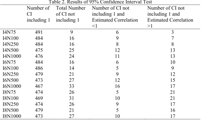
Table2 summarizes the results of 95 percentage confidence interval test. With a 95%
confidence interval, we would expect that about 25 confidence intervals out 500 samples for
each model would not include the correlation of 1.
Table 2. Results of 95% Confidence Interval Test Number of
CI
including 1
Total Number of CI not including 1
Number of CI not including 1 and Estimated Correlation <1
Number of CI not including 1 and Estimated Correlation >1
I4N75 491 9 6 3
I4N100 484 16 9 7
I4N250 484 16 8 8
I4N500 475 25 12 13
I4N1000 476 24 11 13
I6N75 484 16 6 10
I6N100 486 14 5 9
I6N250 479 21 9 12
I6N500 473 27 12 15
I6N1000 467 33 16 17
I8N75 474 26 5 21
I8N100 469 31 10 21
I8N250 474 26 9 17
I8N500 479 21 5 16
I8N1000 473 27 10 17
As we can see from Table 2, when the sample size increases, the confidence interval test
method generally performs better. For all three model specifications with sample size of 250,
500, or 1000, the total numbers of confidence interval not including 1 are all not significantly
different from the expected number, 25. Using Bonferroni correction, I tested whether the
numbers for each model specification are significantly different from 25 and the results are
not significant except for model I4N75.
Within confidence intervals that do not include one, there are two situations: one is that the
estimated correlation itself is smaller than one and the other is it is greater than one. For the
the correct model. The values in this column range from 5 to 12 and do not appear to be
affected by sample size and model complexity. In the last column of table 2, it is the number
of cases that estimated correlation is greater than one and the corresponding confidence
interval does not cover 1. One thing special about Mplus software is that instead of forcing
the correlation to be one during the estimation; it allows such improper solution and gives a
warning message. In this study, having a correlation greater than 1 and a confidence interval
not including 1 is actually an indicator of an incorrect model. In other words, the cases in the
third column, as well as the cases in the first column, all point to the one-factor model as the
correct model, which is the model I used to generate the data. Thus, if we consider the cases
where the estimated correlation is greater than one and the corresponding confidence interval
does not include one as identifying the correct model, then in all the models and sample sizes
considered, the 95 percentage confidence interval test appears to be too conservative when
testing whether the correlation between two constructs is one or not. Same conclusion can be
drawn based on the results of 99 percentage confidence interval test.
6.2 P-Value of LRT/VTT for Nested Models
In this subsection, I look into the p-values of likelihood ratio test and vanishing tetrads test
for nested models. My main concern is the accuracy of the p-value compared to what it
should be at a given type I error. To make the finding comparable with the one from
confidence interval test, I chose to have a Type I error of 0.05. Thus, here I investigate
whether only 5 percentages of all tests (25 tests) are significant for each of these two test
Table 3. Number of P-Value below 0.05 significant level for Nested Test Number of P-Value below 0.05 significant level for Nested Test
LRT VTT
I4N75 22 22
I4N100 28 22
I4N250 20 15
I4N500 27 25
I4N1000 26 22
I6N75 22 1
I6N100 22 4
I6N250 22 8
I6N500 29 16
I6N1000 32 27
I8N75 32 0
I8N100 32 0
I8N250 25 5
I8N500 17 5
I8N1000 24 17
The second column of table 3 is the number of cases that have a p-value less than 0.05 for
the nested likelihood ratio test. Overall, the likelihood ratio test for nested model performs
reasonably well in this study. Except for some large deviation from the expected value in
certain models (I6N1000, I8N75, I8N100, and I8N500), the number of cases with p-value
below 0.05 is pretty close to 251. Its performance does not seem to be influenced by the small
sample size, contrary to what I had expected. The model complexity has some influence as
the models with too low or too high a number of less than 0.05 P-value all happened in the
group with 6 and 8 observed indicators.
The results of vanishing tetrads test for nested models in third column of table 3 show that
it performs fine under the simple model structure. Among the five 4-indicator models, one of
them has exactly 25 cases with less than 0.05 P-value; three of them have 22 such cases,
which is very close to the expected value. However, the vanishing tetrads test does not do
1 For a sample size of 500, the chi-square test shows that a value below 15 or above 35 is significantly different
well for the 6-indicator and 8-indicator models. Other than the two models with 1000 sample
size, the numbers of significant test (with a less than 0.05 P-value) are far below what should
be expected. This is especially true for the 8-indicator model where the model with sample
size of 75 and 100 do not have any test that is significant. Those results suggest that when
testing the dimensionality of theoretical constructs, vanishing tetrads test for nested model
tends to perform poorly when the complexity of the model is high and the sample size is
relatively small.
Based on table 3, we can compare the performance of likelihood ratio test and vanishing
tetrads test for nested models. Both tests did well for the models with 4-indicator model,
regardless of the sample size. But for the more complicated model type, likelihood ratio test
performs much better than the vanishing tetrads test.
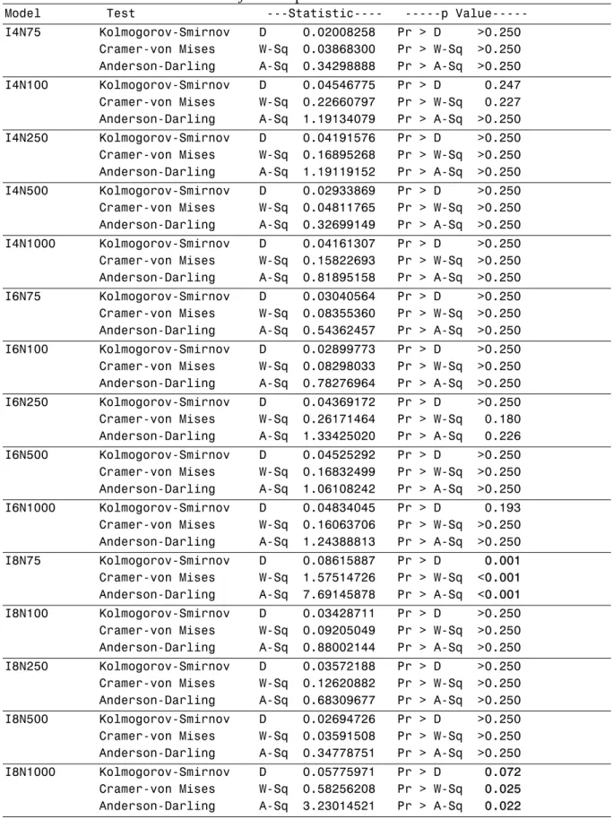
6.3 Distribution of Chi Square Difference
Though in section 6.2 we see that likelihood ratio test does better than the vanishing
tetrads test with regard to how many cases having a significant p-value compared with how
many should be; we still need to further study the entire distribution of the likelihood ratio
test statistics and the vanishing tetrads test statistics resulted from the test of nested models,
which should approximately follow a chi square distribution with 1 degree of freedom. There
is the possibility that the difference may behave well below certain significant level, 0.05 in
this case, it may not follow the chi square distribution as a whole. Since the chi-square
distribution is a special case of the gamma distribution with shape parameter k = n / 2 (n is
the degree of freedom) and scale parameter 2. I conducted Kolmogorov-smirnov test,
Cramer-von Mises test, and Anderson-darling test in SAS with PROC CAPACITY procedure
tetrads test statistics is a chi-square distribution. Those results are present in table 4 and table
5 separately.
The results in table 4 show that for the models with 4 and 6 observed indicators, the
likelihood ratio test statistics all follow the chi-square distribution with 1 degree of freedom.
Across various sample sizes, the p-values for most tests are greater than 0.25 and the lowest
p-value is 0.18, which is still much greater than the commonly used significance level (0.05
and 0.10). For the 5 models with 8 indicator variables, the test results are mixed. All three
tests for model with sample size of 100, 250, and 500 are not significant, with the p-values
greater than 0.25. However, for model with sample size of 75, three tests are all highly
significant with the p-values less than 0.001. This indicates that the test statistics does not
follow a chi-square distribution. Also, for the model with sample size of 1000, the p-values
are 0.072, 0.025, and 0.022, respectively, for those three tests. So we would also reject the
null hypothesis that the test statistics follow a chi-square distribution with one degree of
freedom. The latter case is not expected since the likelihood ratio test should perform better
with large sample size. To make sure that this is just one extreme case, I randomly selected
several other seeding values to generate the data and conducted the analysis. All the resulted
likelihood ratio test statistics follow a chi-square distribution with one degree of freedom at
the 0.05 level of significance. So it appears that the performance of likelihood ratio test for
nested model is affected by small sample size and model complexity. In addition, since all
tests are not significant for 4-indicator and 6-indicator models while two groups of tests for
8-indicator model are, one needs to be more cautious about the performance of likelihood
Table 4. Tests Results for whether Likelihood Ratio Test Statistics for Nested Models Follow a 1 d.f. Chi-Square Distribution
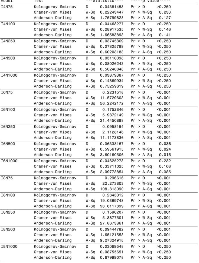
Table 5. Tests Results for whether Vanishing Tetrads Test Statistics for Nested Models Follow a 1 d.f. Chi- Square Distribution
Table 5 summarizes the test result for the vanishing tetrads test statistics. For the models
with 4 observed variables, the p-values range from 0.127 to greater than 0.25. So it means
that we can not reject the null hypothesis that the test statistics for all five sample size are a
chi-square distribution with 1 degree of freedom. It also should be noted that when the
sample sizes increases, so does the p-value for Anderson-Darling test, which may suggest
that the vanishing tetrads test works better with large sample size. For the models with 6 or 8
observed variables, all those tests are significant at the 0.05 level except those two models
with sample size of 1000. Among the five 6-indicator models, the p-values of the tests of
those three models with relatively small sample sizes are all below 0.001. For model I6N500,
the p-values increase to 0.036, 0.024, and 0.015, but are still significant at 0.05 level, leading
to the rejection of null hypothesis. For the model I6N1000, the p-values are 0.232, 0.108, and
0.085. Though they are greater than 0.05, one still would be significant at 0.10 level while
another is very close.
The patterns also hold for the model with 8 observed variables. The hypothesis of the test
statistics follow a chi-square distribution with one degree of freedom all got rejected with
p-value less than 0.001. However, three tests for model I8N1000 all have p-p-value greater than
0.25, thus failing to reject the null hypothesis. Overall, the vanishing tetrads test for nested
models performs all right when the number of observed variable is small. In the case of
model with more indicators, the test only does well when the sample size is large. These
results are consistent with those from the simulation study conducted by Bollen and Ting
(1998). So it seems that both the model complexity and the sample size have an effect on the
performance of the vanishing tetrads test. Bollen and Ting (1998) developed a bootstrapping
procedure in the study, their results show the procedure generally is more accurate than using
the chi-square distribution to compute the p-value of the test statistic in small to moderate
sample sizes with a moderate to large number of observed variables.
7. DISCUSSION AND CONCLUSION
7.1 Main Findings
A main goal of this study was to empirically evaluate the performance of the likelihood
ratio test, confidence interval test, and vanishing tetrads test for testing the dimensionality of
a theoretical construct. This is a very important issue to better understand considering the
significance of the dimensionality issue to social science research—misspecification of the
dimension would lead to either multicollinearity problem for model estimation or omission of
key variables related to the construct.
One major reason for the relatively few empirical examples of testing dimensionality in
stead of using exploratory factor analysis to determine the number of factors underlying data
in social science might be that most researchers are not sure of what tests are available and
which test one should use. One of the assumptions of the most commonly used likelihood
ratio test is violated when testing whether the correlation between two constructs is one or
not. And to my knowledge, no previous study has been conducted to examine its
performance under the SEM context. The relatively new vanishing tetrads test and
confidence interval test also provide possible alternatives for LRT. In this study, drawing on
statistical theory and prior research, I empirically assess those three tests’ performance using
data generated from Monte Carlo simulations. Experimental conditions included 30 different
not experience any non-convergence problem, which might be due to the fact that the
simulation and estimation was conducted for relatively simple model structure. The test
results were presented in previous section.
For the confidence interval test of dimensionality, overall it appears to be too conservative:
when I count the cases where the correlation estimate is greater than one and the
corresponding confidence interval does not include one as accepting of the true model, the
number of tests that falsely reject the true model is much lower than what one should expect
given a certain level of significance. Generally this test method performs relatively better
when the sample size is large. However, the test becomes less accurate when the number of
indicators increases in the model.
The likelihood ratio test for nested models appears to be doing well. It does not show
obvious signs of impact of the violation of boundary condition when testing for
dimensionality. The number of tests that incorrectly concludes the two-factor model is the
true model is pretty close to the expected value at the 0.05 LEVEL of significance. And the
accuracy of the test is influenced by the model complexity but not small sample size. When I
examined the whole distribution of the likelihood ratio nested test statistics, most of them
prove to follow a Chi-square distribution with 1 degree of freedom. Only in two cases,
(model I8N75 and model I8N1000), the null hypothesis were rejected at the 0.05 level
significance. All these findings indicate that despite the existence of boundary condition, the
likelihood ratio test for nested models functions reasonably well in this study with few minor
problems.
As a relatively new method for testing model fit, the performance of vanishing tetrads tests
for the models with 4 observed variables, correctly identifying expected number of the true
model at the selected p-value. However, for the model with 6 and 8 observed variable, the
test only performs well for the models with the largest sample size. For other models, the
number of misidentified cases is greatly lower than what it should be. The same patterns hold
when I check the whole distribution of the vanishing tetrads test statistics. All the chi-square
differences from models with 4 observed variables follow a chi-square distribution with 1
degree of freedom. But again, for the models with 6 or 8 observed variables, with the
exception of two models with sample size of 1000, all other models’ test statistics turned out
be significant at the 0.05 level. So in general, the vanishing tetrads tests for nested models
did all right when the number of observed variable is small. However, when dealing with
more complex model and small sample size, the test appears to be too conservative for the
given level of significance and the test statistics does not follow the expected distribution
form in this study. These are the same pattern of results as in Bollen and Ting (1998), in
which they developed a bootstrap approach for computing the p-value of the test statistics in
small to moderate sample size.
7.2 Limitations and Future Research
An inherent limitation to any Monte Carlo simulation study is that the results of the study
are necessarily limited to the parameterization of the models and conditions under study, and
care should be taken when generalizing my findings presented here since findings may differ
with variations in factors such as model complexity, model parameterization, and degree of
misspecification. However, I took great care in the design of my simulation experiment
these findings could be generalized to similar types of CFA models testing univariate vs.
bivariate dimensions.
One thing that should be noted for the vanishing tetrads test is that there is not simply a
single set of nonredundant vanishing tetrads for a model, but rather many possible
combinations. As a result, the test statistics obtained through the vanishing tetrads test SAS
Macro would change each time depending on which set of vanishing tetrads the nested test
uses. The benefit for this is the program could allow the researchers to assess the robustness
of their finding. However, in this study both the 1-factor and 2-factor models fit the data
relatively well so the difference between those chi-squares is sometimes very small. As a
result, the changing vanishing test tetrads test statistics could affect the results that I
presented in section 6.2 and 6.3. In addition, the SAS Macro could not properly conduct the
nested test for the 4-indicator models due to some unsolved bug. I have to get around this by
doing the vanishing tetrads test separately for the 1-factor and 2-factor and then do the nested
models test, which might have some effect on the final results.
Another limitation of my study is that I examined only data generated from a multivariate
normal distribution. Prior research has indicated that it is important to also consider
non-normally distributed data (e.g., Muthén & Kaplan, 1985, 1992), but an examination of this
was beyond the scope of the current project. Given that non-normal distributions are a
significant problem in social science research (e.g. Micceri, 1989), much can be learned
about the performance of those three tests with nononormally distributed data. Finally, all the
variables in this study are continuous. Considering more and more researches are involved
with censored, ordinal, and dichotomous variables, it would be interesting to look into those
should warrant some caution in over generalizing from results of this study, but I think my
findings provide an important first glimpse into the empirical testing of dimensionality and I
hope that it could serve as a starting point for future research on this important topic of
REFERENCE
Aitchison, J. and S. D. Silvey. 1958. “Maximum-likelihood estimation of parameters subject to restraints.” The annals of mathematical statistics 29:813-828.
Anderson, J. C. and D.W. Gerbing. 1984. “The effect of sampling error on convergence, improper solutions and goodness of fit indices for MLE CFA.” Psychometrika
49:155-173.
Andrews, Donald W. K. 2001. “Testing when a parameter is on the boundary of the maintained hypothesis.” Econometrica 69:683-734.
Asparouhov, T. (2004). “Weighting for unequal probability of selection in multilevel modeling.” Mplus Web Notes: No. 8.
Asparouhov, T. (2005). “Sampling weights in latent variable modeling.” Structural Equation Modeling 12:411-434.
Bishop, Y. M., T. S. Fienberg, and P. Holland. 1975. Discrete Multivariate Analysis.
Cambridge, MA: MIT Press.
Blalock, Hubert M., Jr. 1963. “Correlated independent variables: the problem of multicollinearity.” Social Forces 42:233-237.
Blau, Perter M. 1967. “The hierarchy of authority in organization.” American Journal of Sociology 73:453-467.
Bollen, Kenneth A. 1979. “Political democracy and the timing of development.” American Sociological Review 44:572-587.
—. 1980. “Issues in the comparative measurement of political democracy.” American Sociological Review 45:370-390.
—. 1989. Structural Equations with Latent Variables. New York: Wiley.
—. 1990. “Outlier screening and a distribution-free test for vanishing tetrads.” Sociological Methods & Research 19:80-92.
Bollen, Kenneth A. and Burke D. Grandjean. 1981. “The dimension(s) of democracy: Further issues in the measurement and effects of political democracy.” American Sociological Review 46:651-659.
Bollen, Kenneth A. and K. F. Ting. 1993. “Confirmatory tetrad analysis.” Pp. 147-176 in
Sociological Methodology, vol. 23, edited by P. V. Marsden. Cambridge, MA:
—. 1998. “Bootstrapping a test statistic for vanishing tetrads.” Sociological Methods & Research 27:77-102.
—. 2000. “A tetrad test for causal indicators.” Psychological methods 5:3-22.
Bourdieu, Peirre. 1983. “Forms of capital.” Pp. 241-258 in Handbook of theory and research for the sociology of education, edited by J. G. Richardson. New York: Greenwood
Press.
Browne, M. W. 1984. “Asymptotic distribution free methods in analysis of covariance structures.” British journal of mathematical and statistical psychology 37:62-83.
Chant, D. 1974. “On asymptotic tests of composite hypotheses in nonstandard conditions.”
Biometrika 61:291-298.
Chen, Feinian, Kenneth A. Bollen, Pamela Paxton, Patrick J. Curran, and James B. Kirby. 2001. “Improper solutions in structural equation models.” Sociological Methods & Research 29:468-508.
Chernoff, Herman. 1954. “On the distribution of the likelihood ratio.” The annals of mathematical statistics 25:573-578.
Child, John. 1972. “Organization structure and strategies of control: a replication of the Aston studies.” Administrative science quarterly 17:163-177.
Coleman, James S. 1988. “Social capital in the creation of human capital.” American Sociological Review 94:S95-S120.
Cox, D.R. and David V. Hinkley. 1974. Theoretical Statistics. New York: Chapman and Hall.
Curran, Patick J., Kenneth A. Bollen, Fennian Chen, Pamela Paxton, and James B. Kirby. 2003. “Finite sampling properties of the point estimates and confidence intervals of the RMSEA.” Sociological Methods & Research 32:208-252.
Curran, Patrick J., Kenneth A. Bollen, Pamela Paxton, James Kirby, and Feinian Chen. 2002. “The noncentral chi-square distribution in misspecified structural equation models: Finite sample results from a Monte Carlo simulation.” Multivariate Behavioral Research 37:1-36.
Curran, P. J., S. G. West, and J. Finch. 1996. “The robustness of test statistics to non-normality and specification error in confirmatory factor analysis.” Psychological methods 1:16-29.
Curran, Patrick J., Stephen G. West, and John F. Finch. 1996. “The robustness of test statistics to nonnormality and specification error in confirmatory factor analysis.”
Cutright, Phillips. 1963. “National Political development.” American Sociological Review
28:253-264.
Feder, Paul I. 1968. “On the distribution of the log likelihood ratio test statistic when the true parameter is “near” the boundaries of the hypothesis regions.” The annals of
mathematical statistics 39:2044-2055.
Flora, D.B. & Curran P.J. (2004). “An empirical evaluation of alternative methods of
estimation for confirmatory factor analysis with ordinal data.” Psychological Methods,
9:466-491.
Gerbing, D.W. and J. C. Anderson. 1985. “The effect of sampling error and model
characteristics on parameter estimation for maximum likelihood confirmatory factor analysis.” Multivariate Behavioral Research 20:255-271.
Glymour, C., R. Scheines, P. Spirtes, and K. Kelly. 1987. Discovering causal structure.
Orlando, FL: Academic Press.
Hall, Richar H. 1963. “The concept of bureaucracy: an empirical assessment.” American Journal of Sociology 69:32-40.
Hipp, John R., Daniel J. Bauer, and Kenneth A. Bollen. 2005. “Conducting tetrad tests of model fit and contrasts of tetrad-nested models: A new SAS Macro.” Structural Equation Modeling 12:76-93.
Hipp, John R. and Kenneth A. Bollen. 2003. “Model fit in structural equation models with censored, ordinal, and dichotomous variables: Testing vanishing tetrads.”
Sociological Methodology 33:267-305.
Hox, J.J. 1995. “AMOS, EQS, and LISREL for windows: A comparative approach.”
Structural Equation Modeling 1:79-91.
Hu, L. and P.M. Bentler. 1998. “Fit indices in covariance structure modeling: Sensitivity to under parameterized model misspecification.” Psychological methods 3:424-453.
Huber, P. J. 1967. “The behavior of maximum likelihood estimates under nonstandard conditions.” Pp. 221-233 in Proceedings of the Fifth Berkeley Symposium on Mathematical Statistics and Probability, vol. 1.
Jackman, Robert W. 1975. Politics and Social Equality: A comparative analysis. New York:
Wiley.
Kelly, T. L. 1928. Crossroads in the mind of man: A study of differentiable mental abilities.
Stanford, CA: Stanford University.
Kohn, Melvin. 1976. “Occupational structure and alienation.” American Journal of Sociology
82:111-130.
MacIntosh, R. & Hashim, S. (2003). “Converting MIMIC model parameters to IRT parameters in DIF analysis.” Applied Psychological Measurement 27:372-379
Marsh, H. W., K. T. Hau, J. R. Balla, and D. Grayson. 1998. “Is more ever too much? The numer of indicators per factor in confirmatory factor analysis.” Multivariate Behavioral Research 33:181-220.
Matsueda, R.L. and W.T. Bielby. 1986. “Statistical power in covariance structure models.”
Sociological Methodology 16:120-158.
McDonald, James B. and Yexiao Xu. 1992. “An empirical investigation of the likelihood ratio test when the boundary condition is violated.” Communications in statistics--Simulation 21:879-892.
Micceri, T. 1989. “The unicorn, the normal curve, and other improbable creatures.”
psychological bulletin 105:156-166.
Muthen, B. O. and D. Kaplan. 1992. “A comparison of some methodologies for the factor analysis of non-normal Likert variables.” British journal of mathematical and statistical psychology 38:171-189.
Muthen, B. O. and D. Kaplan. 1995. “A comparison of some methodologies for the factor analysis of non-normal Likert variables: A note on the size of the model.” British journal of mathematical and statistical psychology 45:19-30.
Narayan, Deepa and Michael F. Cassidy. 2001. “A dimensional approach to measuring social capital: Development and validation of a social capital inventory.” Current Sociology
49:59-102.
Paladam, M. 2000. “Social capital: One or Many?--Definition and Measurement.” Journal of Economic survey 14:629-653.
Parker, Robert N. 1983. “Measuring social participation.” American Sociological Review
48:864-873.
Paxton, Pamela. 1999. “Is social capital declining in the United States? A multiple indicator assessment.” American Journal of Sociology 105:88-127.
“Monte Carlo experiments: design and implementation.” Structural Equation Modeling 8:287-312.
Portes, Alejandro. 1998. “Social Capital: its origins and applications in modern sociology.”
Annual Review of Sociology 22:1-24.
Pugh, D. S., D. J. Hickson, C. R. Hinings, and C. Turner. 1968. “Dimensions of organization structure.” Administrative science quarterly 13:65-105.
Putman, R. 2001. Bowling alone: The collapse and revival of the American community. New
York: Simon & Achuster Inc.
Rao, C. R. 1973. Linear Statistical Inference and its Application. New York: Wiley.
Reimann, Bernard C. 1973. “On the dimensions of bureaucratic structure: An empirical reappraisal.” Administrative science quarterly 18:462-476.
Samuel, Yitzhak and Bilha F. Mannheim. 1970. “A multi-dimensional approach toward a typology of bureaucracy.” Administrative science quarterly 15:216-228.
Seeman, Melvin. 1959. “On the meaning of Alienation.” American Sociological Review
24:783-791.
Self, Steven G. and Hung-Yee Liang. 1987. “Asymptotic properties of maximum likelihood estimators and likelihood ratio test under nonstandard conditions.” Journal of the American Statistical Association 82:605-610.
Shapiro, Alexander. 1985. “Asymptotic distribution of test statistics in the analysis of moment structures under inequality constraints.” Biometrika 72:133-144.
Siemsen, Enno and Kenneth A. Bollen. 2005. “The small sample robustness of least absolute deviation estimation in structural equation modeling.” chapel hill.
Stram, Daniel O. and Jae Won Lee. 1994. “Variance components testing in the longitudinal mixed effects model.” Biometrics 50:1171-1177.
Velicer, W.F. and J. L. Fava. 1998. “Effects of variable and subject sampling on factor pattern recovery.” Psychological methods 3:231-251.
Vu, H. T. V. and S. Zhou. 1997. “Generalization of likelihood ratio tests under nonstandard conditions.” The Annals of Statistics 25:897-916.
Waller, N. G. 1993. “Software review: seven confirmatory factor analysis programs.”