Solutions to the nonlinear Schrodinger equation with Dirac mass initial data

(1)

Solutions to the Nonlinear Schrodinger Equation with Dirac

Mass Initial Data

Jason Newport

A dissertation submitted to the faculty of the University of North Carolina at Chapel Hill in partial fulfillment of the requirements for the degree of Doctor of Philosophy in the Department of Mathematics.

Chapel Hill 2008

Approved by

(2)

ABSTRACT

JASON NEWPORT: Solutions to the Nonlinear Schrodinger Equation with Dirac Mass Initial Data

(Under the direction of Kenneth T-R McLaughlin)

(3)

(4)

ACKNOWLEDGEMENTS

(5)

LIST OF FIGURES

(8)

CHAPTER 1

Introduction

The goal of this paper is to analyze solutions of the defocussing nonlinear Schrodinger (NLS) equation with Dirac mass intial data:

iϕt+ϕxx−2|ϕ|2ϕ= 0 (1.1)

ϕ(x, t= 0) =δ(x).

(1.2)

In chapter 1.1 we investigate the linear Schrodinger equation with Dirac mass initial data:

iϕt+ϕxx = 0 (1.3)

ϕ(x, t= 0) =δ(x).

(1.4)

We will study this via a straightforward regularization which will motivate the regular-ization that we need to use when solving the nonlinear problem.

(9)

In chapter 3 we will find the scattering data corresponding to Dirac mass initial data. We will formulate a Riemann Hilbert Problem (RHP), and see why the theory breaks down with constant scattering data. Then we introduce a regularization similar to the one we used in section 1.1.

In chapter 4 we preform asymptotic calculations on the RHP with the regularized reflection coefficient to find the asymptotic behaviour of the potential.

In chapter 5 we find a connection between long time asymptotics and sequences of initial data that converge to a Dirac mass.

1.1. Linear Schrodinger Equation

To motivate the need for a regularization of the scattering data in the nonlinear case, we will start with the simpler linear equation. The Linear Schrodinger Equation is defined as

(1.5) iqt+qxx = 0,

where we have chosen the initial data as the Dirac mass:

(1.6) q(t= 0, x) =δ(x).

Using the fourier transform

F{f}(k) = ˆf(k) = √1

2π

Z ∞

−∞

(10)

we see that, formally, the solution to our equation should be

(1.7) q(t, x) = 1

2π

Z ∞

−∞

eikx−ik2tdk.

However, the integrand in (1.7) is purely oscillitory, and we must decide upon a proper interpretation of the integral.

At this point we introduce a regularization to our transformed data to ensure that the inverse transform of our initial data converges. Let

(1.8) qˆ₀ = √1

2πe

−k2 .

Now, our solution (1.7) becomes

q(t, x) = 1 2π

Z

R

eikx−ik2t−k2dk.

Straightforward calculations yield:

(1.9) q(x, t) = 1 2πe

ix2

4t e−i π

4

Z

R

e−(t−i)z2dz.

In the limit as →0 we find the solution is

(1.10) q(t, x) = 1

2√πte

−iπ

4e

ix2

4t .

Consider the asymptotics of our solution, as t → 0. We will show that it converges weakly to the Dirac delta. Leth(x) be any smooth test function, and define

I(x, t) =

Z

R

q(x, t)h(x)dx= 1 2√πte

−iπ

4

Z

R

eix 2

(11)

Ast →0, the dominant contribution from the integral is atx= 0. The stationary phase method yields

I(x; s) = h(0) +O(√t).

Thus, our solution converges weakly to the Dirac delta function.

Remark: We have shown that if →0 the formula (1.9), converges to a Dirac mass as t → 0. A modification of this calculation shows that the order of limits does not matter. Indeed, if the vector (t, ) → 0 in formula (1.9), then the result converges to a Dirac mass as → 0. In the nonlinear case, we will see that we cannot interchange the order of limits.

1.2. Results

Formal considerations in chapter 3 lead us to a one parameter family of reflection coefficients:

r(z, t) = 1 1 +γ−γ2 e

4iz2_t .

For ease of calculation we will choose γ = 1₂. We consider the regularized reflection coefficient

(1.11) r(z, t) = 4

5e

−2z2_+4iz2_t .

Our interest is the behaviour of the solution to the NLS equation with initial data corresponding to (1.11), as→0. The following is our main result, proven in chapter 4.

Theorem 1.2.1. Let ϕ(x, t;) represent the solution to the NLS equation

(12)

0< T1 < T2 <∞ and0< X <∞, the following expansion holds true for all T1 < t < T2 and |x|< X:

ϕ= √1

te

ix2

4t−2iνlog(8t)−2iνeh(z0)

√

π5e

iπ/4−πν/2

4Γ(−iν) +O √

log(),

with ν(z) and h(z) defined in (A.1) and (A.3) respectively.

The meaning of the error term is that there exists a constant C depending on T1, T2 and X so that the error is bounded byC|√(log)2| for all allowable x and t.

Theorem1.2.2. Letr˜(λ)be the reflection coefficient corresponding to the initial data

f(x). Consider initial conditions of the form

ϕ(x, t= 0;) = 1

f

x

,

and let M be a positive constant. Then for all values x and t where |z0| =

−x_4t

≤ M,

the solution has the following asymptotic expansion:

ϕ(x, t;) = √1

te

ix2

4t−iνlog(8t)2iνu(z₀) +O(log)

with

iν(z0) = 1

2πilog 1− |˜r(z0)|

2

.

The function u is defined in terms of its modulus and phase:

|u(z0)|2 =ν/2 =− 1

4πlog(1− |˜r(z0)|

2₎

arg u(z0) = 1

π

Z z0

−∞

log(z0−s)d log(1− |˜r(s)|2) +

π

(13)

Remark: The question which led to the first theorem was ’What is the behaviour of solutions associated with regularizations of constant reflection coefficients.’ The sort of regularizations we considered were in the general class of delta sequences discussed in Theorem 1.2.2. In addition, the method used to prove the two theorems are quite different. The former involves Riemann Hilbert Analysis of the inverse spectral problem, while the latter relies on established long time asymptotics.

A slightly stronger version of Theorem 1.2.2 follows.

Theorem1.2.3. Letr˜(λ)be the reflection coefficient corresponding to the initial data

f(x). Consider iinitial conditions of the form

ϕ(x, t= 0;) = 1

e

−2iαx

fx

,

and let M be a positive real constant. For any constant α∈_R and for all values x and t

where |z0|=

−x_4t

≤M the solution has the following asymptotic expansion:

ϕ(x, t;) =e−2iαx−2iα2t

1 √

te

ix2

4t−iνlog(8t)2iνu(z₀) +O(log)

with

iν(z0) = 1

2πilog 1− |˜r(z0)|

2

.

The function u is defined in terms of its modulus and phase:

|u(z0)|2 =ν/2 =− 1

4πlog(1− |˜r(z0)|

2 )

arg u(z0) = 1

π

Z z0

−∞

log(z0−s)d log(1− |˜r(s)|2) +

π

(14)

1.3. Motivation For Studying Singular Limits of the NLS Equation

We are studying the behaviour of the NLS equation with Dirac mass initial data for several reasons. The scattering and inverse scattering theory found herein is well established. Existence and uniqueness of long time asymptotics are known for initial data in a weighted Sobolev space [4]. The Dirac mass is a distribution that is outside this class of functions. In this paper we find that solutions exist for sequences of initial conditions that converge to a Dirac mass. One interesting part of analysis is that the solutions are not unique.

Another reason we studied these problems is to figure out how the NLS equation regularizes singular data. In order to study this we had to regularize the reflection coefficient and develop the machinery to handle the limit when this smoothing parameter went to zero. Once we had found solutions, one could ask what happened when t →0. The limit as the smoothing parametertends to zero does not necessarily commute with the limit when t→0.

(15)

CHAPTER 2

Scattering and Inverse Scattering Theory

In this chapter we will study the defocusing nonlinear Schrodinger equation:

iϕt+ϕxx−2|ϕ|2ϕ= 0

with Schwartz class initial data.

The scattering and inverse scattering theory we will discuss is a nonlinear version of the Fourier method for solving linear partial differential equations. We find scattering data via the direct spectral transform. This scattering data has a very simple evolution in time. In order to reconstruct the solution at later times we must go from the evolved scattering data back to the potential, which is achieved using Riemann Hilbert methods. This scattering and inverse scattering theory have been studied in great detail; in [1] and [6], for example.

The Lax pair associated with the NLS equation is the pair of linear operators:

(2.1) L=iσ3

∂ ∂x +i

   

0 −ϕ

ϕ 0

(16)

(2.2) B = 2zI ∂ ∂x +i

   

−|ϕ|2 _ϕ x

−ϕx |ϕ|2

   

.

If a 2×2 matrix functionψ =ψ(x, t, z;ϕ) exists so that

(2.3) Lψ =zψ

(2.4) ∂

∂tψ =Bψ,

the compatibility of partial derivatives implies that ϕ solves the NLS equation.

Letz ∈_C+ and assumet = 0. Then the differential equation

iσ3

∂ ∂xΨ +i

   

0 −ϕ

ϕ 0

   

Ψ = zΨ,

together with the asymptotic conditions:

(2.5) Ψ(x, z)

   

eizx ₀ 0 e−izx

   

→I asx→ ∞;

and

(2.6) Ψ(x, z)

   

eizx 0 0 e−izx

   

bounded as x→ −∞.

possesses a unique solution.

We will use the notation

eizxσ3 ₌

   

eizx ₀ 0 e−izx

(17)

Define

(2.7) M = Ψ(x, z)eizxσ3

so that

(2.8) M →I when x→ ∞.

2.1. Potentials with Compact Support

In this section we will assume that supp(ϕ) = (xl, xr). Many of the analytical issues are greatly simplified in this setting. Our goal is to provide a well-known (see [1]) description of the reflection coefficient.

We will begin by building unique solutions to (2.3) and (2.4) at t = 0. For x > xr, (2.3) simplifies to

iσ3

∂

∂xΨ =zΨ.

Thus,

Ψ(x, z) =eizxσ3_C ₌

   

eizx 0 0 e−izx

   

   

c11 c12

c21 c22

   

,

for x > xr, where the matrix C is constant in x.

Let z ∈_C+. By the asymptotics in (2.5), we know c22 =c11 = 1, c12 = 0. However,

c21 is not determined. If we do a similar analysis as x→ −∞, we find that

Ψ(x, z) =

   

e−izx 0 0 eizx

   

   

d11 d12

d21 d22

   

(18)

In order for Ψ to be bounded, we need d21 = 0. However, d11, d12, d22 have yet to be determined. Thus, we have

(2.9) Ψ(x, z) =e−izxσ3

   

1 0

c21 1

   

x > xr

(2.10) Ψ(x, z) =e−izxσ3

   

d11 d12 0 d22

   

x < xl.

Forz ∈_C−, a similar analysis shows that our solution is

(2.11) Ψ(x, z) =e−izxσ3

   

1 ˆc12 0 1

   

x > xr

(2.12) Ψ(x, z) =e−izxσ3

   

ˆ

d11 0 ˆ

d21 dˆ22

   

x < xl.

Proving Ψ exists in (xl, xr) follows from standard ODE theory. We find that there is a unique c21(z) that forces d21= 0.

The function Ψ has boundary values asz tends towards the real axis. Let

Ψ+ = lim Im(z)&0Ψ

(19)

These both exist since Ψ(z) is analytic off the real axis and the support of ϕis compact. Now we have 2 fundamental solutions to the same ODE on the real axis, and so they must be related as follows:

(2.13) Ψ+(x, z) = Ψ−(x, z)

   

v11 v12

v21 v22

   

(z).

Forx > xr, using (2.9) and (2.11), we get

   

1 0

c21 1

    =    

1 ˆc12 0 1        

v11 v12

v21 v22

   

(ξ).

Simplifying, we get

(2.14)

   

1−c21ˆc12 −ˆc12

c21 1

    =    

v11 v12

v21 v22

   

(z).

The mapping ϕ(x)−→ c12(z) is our nonlinear transform. The function c21 is called the reflection coefficient and is denotedr(z, t).

2.2. Evolution in Time

(20)

in appendix A.2. See also [4]. It should be noted that due to this theory, we know the solution Ψ (and therefore,M) is differentiable.

Straightforward algebra shows that _∂t∂L= [B L]. Recall, LΨ = zΨ with the asymp-totic conditions (2.5) and (2.6). Differentiating with respect to t, we obtain

∂

∂t(zΨ) =BLΨ−LBΨ +LΨt.

Rearranging, yields

L(Ψt−BΨ) =z(Ψt−BΨ).

Therefore, both Ψt−BΨ, and Ψ are eigenfunctions of L with the same eigenvalue. Thus they are related by:

Ψt−BΨ = ΨE,

where E is a matrix whose entries are constant in x. We can rewrite this equation in terms of M:

Mt−BM =M e−izxσ3Eeizxσ3.

In A.2 we show some properties of M, including the fact that it is bounded. It is easily shown that, M−1(Mt−BM) is bounded as x→ ±∞. In addition, it follows that

det M = 1. Therefore, E12 = E21 = 0. Using the asymptotics for M, derived from the asymptotics for Ψ (2.5) and (2.6), we find that

M−1(Mt−BM)→2iz2σ3,

(21)

Thus, we find E = 2iz2_σ

3. In terms of Ψ, we have

(2.15) Ψt−BΨ = 2iz2σ3Ψ.

Differentiating (2.13) with respect to time, and using (2.15), we find

Vt = [V , E]

= 2iz2[V , σ3].

Using the definition (2.13) of the jump matrix, we have

(2.16) r(z, t) =e4iz2tr(z,0) =e4iz2tv12 for z ∈R.

A symmetry of the Lax pair allows us to write the jump matrix for Ψ as

(2.17) V =

   

1− |r|2 ₋_r₍_{z, t}₎

r(z, t) 1

   

.

2.3. Formulation of RHP and Inverse Scattering Theory

We have computed the reflection coefficient and how it evolves in time. We want a procedure to reconstruct the potential as it evolves with the NLS equation. We use the inverse scattering transform solved with Riemann Hilbert approach. For this section we assume M exists and is differentiable. The proof that M exists relies heavily on the knowledge of the Lax pair and the function ϕ, and can be found in appendix A.2.

We know M is analytic off of the real axis and that it has identity asymptotics as

(22)

on the real axis. Using the jump matrix for Ψ and the definition of M, (2.17) and (2.7), we can find the jump relation for M:

M+(z) = M−(z)

   

1− |r|2 ₋_r₍_z₎_e−2izx−4iz2_t r(z)e2izx+4iz2_t

1

   

z ∈_R.

These properties can be combined to formulate a Riemann Hilbert Problem: We wish to find a matrix M that has the following properties:

M(z) is analytic off the real axis

M(z) =I+ M1

z + M2

z2 +· · · z → ∞

M+(z) =M−(z)

   

1− |r|2 ₋_r₍_z₎_e−2izx−4iz2_t r(z)e2izx+4iz2t ₁

   

z ∈_R.

If we can find such an M, the solution to the NLS equation is embedded in M as shown in the following theorem.

Theorem 2.3.1. Assume ϕ is Schwartz class for t = 0. Then the solution ϕ to the

NLS equation is:

ϕ= 2i(M1(x, t))12,

where (M1)12 is the upper right entry of the first moment of M as z → ∞.

Proof. We know that M solves the differential equation

∂

(23)

where

Q=

   

0 ϕ

ϕ 0

   

.

If M =I+z−1M1+· · ·, then

z−1 ∂

∂xM1+· · ·=iz[I+z

−1

M1+· · · , σ3] +Q(I+z−1M1+· · ·).

Solving for the leading order term yields Q = −i[M1, σ3]. In terms of the matrix entries:

   

0 ϕ

ϕ 0

   

= 2i

   

0 (M1)12 −(M1)21 0

   

.

Thus,

ϕ= 2i(M1)12= 2i lim

z→∞z(M(z)−I)12.

Remark: Theorem 2.3.1 is a well known fact and is true under weaker conditions on the potential. In [4] Deift and Zhou require only that the intial data be in the weighted sobolev spaceH1,1_.

(24)

(25)

CHAPTER 3

Obtaining the Reflection Coefficient with Dirac Mass Initial

Data

Our goal is to find the reflection coefficient corresponding to NLS equation with Dirac mass initial data:

iϕt+ϕxx−2|ϕ|2ϕ= 0 (3.1)

ϕ(x, t= 0) =δ(x),

where a is a constant.

Seeking a solution to equation (2.3), satisfying (2.5) and (2.6), with a Dirac mass potential is somewhat problematic. At t = 0, we have ϕ=ϕ=δ(x). For this reason, Ψ will have a jump discontinuity at x = 0. We must append a rule for how a Dirac mass acts on a function with a jump discontinuity. We will proceed formally by imposing rules to evaluate

Z

R

Ψδ(x)dx.

We will use a weighted average of limiting values from the left and right. Using (3.3), we define

(3.2)

Z

R

Ψδ(x)dx=γ

lim x→0−Ψ(x)

+ (1−γ)

lim x→0+Ψ(x)

(26)

Now we will compute our reflection coefficient. Note that supp(ϕ(x, t = 0)) = {0}. Thus, (2.10) and (2.9) become

Ψ(x, z) =e−izxσ3

   

1 0

c21 1

   

x >0

Ψ(x, z) =e−izxσ3

   

d11 d12 0 d22

   

x <0.

For brevity, let

C =     1 0

c21 1

    D=    

d11 d12 0 d22

   

.

Then Ψ has the following representation:

(3.3) Ψ =e−izxσ3_D₊_H₍_x₎_e−izxσ3₍_C₋_D₎_,

with H being the heavyside function defined as

H(x) =

            

0 x <0

1

2 x= 0

1 x >0.

Supposet= 0. To find our reflection coefficient we integrate the equationLΨ−zΨ = 0 against a test function h(x) over the entire real axis. The weak form of this equation is:

(3.4) −iσ3

Z

R

Ψh0(x)dx−i

Z R    

0 −ϕ

ϕ 0

   

Ψh(x)dx−z

Z

R

(27)

Since we already know Ψ solves this equation for x 6= 0, most of the terms in the equation will cancel. Then (3.4) can be rewritten as

0 = iσ3e−izaσ3(C−D)h(0) +i

Z R    

0 −ϕ

ϕ 0

   

Ψh(x)dx

= h(0)

   

iσ3(C−D) +i

   

−γc21 −γ−(1−γ)d22

γ+ (1−γ)d11 (1−γ)d12

       

This is valid for any test function h, so

   

(1−d11) −d12 −c21 −(1−d22)

    +    

−γc21 −γ−(1−γ)d22

γ+ (1−γ)d11 (1−γ)d12

   

= 0.

We can easily solve these equations for c21, yielding

c21=

1 1 +γ−γ2.

We can consider the Dirac delta function as a limit of piecewise constant functions whose integral is one:

(3.5) q(x) =

       1

δ |x| ≤δ 0 |x|> δ

.

Using the work of DiFranco and McLaughlin in [5], we can find the reflection coef-ficient for initial conditions of the form (3.5). In the limit when δ → 0 the reflection coefficient is a constant:

lim

δ→0r(z, δ) =

e4₋₁

(28)

We can choose γ so that our reflection coefficient matches this limiting case. For sim-plicity, we choose γ = 1₂ yielding our reflection coefficient

(3.6) r(z, t= 0) =c21= 4 5,

as this will not effect the analysis in the upcoming calculations.

Recall the RHP for M. The problem is to find a 2 matrixM that satisfies:

M(z) is analytic off the real axis (3.7)

M(z) = I+ M1

z +

M2

z2 +· · · z→ ∞ (3.8)

M+(z) = M−(z)

   

1− |r|2 ₋_r₍_z₎_e−2izx−4iz2_t r(z)e2izx+4iz2t 1

   

z ∈_R.

(3.9)

Unfortunately, with Dirac mass initial data, this problem is ill-posed. Similar to the linear problem we looked at, our transformed data r(z) = 4₅ is a constant. We know

M →I as z → ∞. However, if we look at the third condition of our RHP, we see that

M+_{, M}− _→ _I _for _z _{→ ∞. But our jump matrix will not converge since} _r _{is constant,} and z ∈_R.

In order to solve our problem, we will introduce a regularization in the same way that we did for the linear case. Let

(3.10) r(z) :=r(z)e−2z2 = 4 5e

(29)

Using this regularization our reflection coefficient now decays as z → ∞, and we can find the solution to our RHP. It is the goal of the next chapter to study the behavior as

→0.

(30)

CHAPTER 4

Asymptotic Analysis of the RHP

In this chapter we will find an explicit approximation for our Riemann Hilbert Prob-lem with regularized data. We will make use of a solution to a similar RHP, solved by Deift and Zhou in [3]. Using a series of explicit transformations, we will show that an equivalent form of our RHP is sufficiently close to theirs. We will then use Neumann series to compute the error.

We will use the Lie algebra notation

λadσ3_v ₌_λσ3_vλ−σ3_,

to make the transformations simpler to read.

Define a RHP with regularized data to be

M(z) is analytic off the real axis (4.1)

M(z) = I+M 1

z +

M 2

z2 +· · · z → ∞ (4.2)

M₊(z) = M₋(z)e(−izx−2iz2t)adσ3

   

1− |r₍_z_)|2 ₋_r₍_z₎

r₍_z₎ ₁

   

z ∈_R.

(4.3)

The solution to the NLS equation is

(4.4) ϕ= 2ilim

(31)

The RHP solved by Deift and Zhou in [3] is:

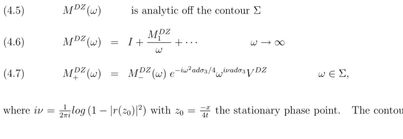
MDZ(ω) is analytic off the contour Σ (4.5)

MDZ(ω) = I +M DZ 1

ω +· · · ω → ∞

(4.6)

M₊DZ(ω) = M₋DZ(ω)e−iω2adσ3/4_ωiνadσ3_VDZ _ω _∈_Σ_,

(4.7)

where iν = _2πi1 log(1− |r(z0)|2) with z0 = −x_4t the stationary phase point. The contour

Figure 4.1. The Contour Σ

Σ is shown in Figure 4.1. The jump matrix is defined as:

VDZ(ω) =

                    

Vr(z0) ω ∈Σ2 ˆ

Vr(z0) ω ∈Σ3 ˆ

Vl(z0) ω ∈Σ5

Vl(z0) ω ∈Σ6 . ,

(32)

As in (4.4), the information we need is in the (1,2) entry of the the first moment of

MDZ at infinity. From their paper,

(4.8) M₁DZ

12=

−i√2πeiπ/4_e−πν/2

r(z0)Γ(−iν)

.

This is the solution to a model RHP, obtained through a series of transformations.

4.1. Transformations to an Equivalent RHP

In this section we will show the explicit transformations we use to find a RHP equiv-alent to ours, which is close to the RHP stated in (4.5) - (4.7).

It will be useful to define V0 as

V0 =

   

1− |r(z)|2 ₋_r₍_z₎

r₍_z₎ ₁

   

.

The jump matrix can be written as V =e−itθadσ3_V

0, where

θ= 2z2+zx

t = 2(z−z0)

2₋₂_z 0.

The stationary phase point is defined to be z0 =−_4tx.

Remark: We will drop the superscript from the reflection coefficient. For the remainder of this chapter it is assumed that we are working with the regularized reflection coefficient.

Now we define two factorizations ofV0:

(33)

with

(4.10) Vl =

   

1 −r(z)

0 1     ,

(4.11) Vr =

   

1 0

r(z) 1

    ; and

(4.12) V0 = ˆVl VˆcVˆr

with

(4.13) Vˆl=

    1 0 r(z) 1−|r(z)|2 1

   

,

(4.14) Vˆc=

   

1− |r(z)|2 ₀ 0 (1− |r(z)|2₎−1

   

,

(4.15) Vˆr =

   

1 −_1−|r(z)|r(z) 2

0 1     .

LetV0 be factored according to:

V0 =

      

VlVr z > z0

ˆ

VlVˆcVˆr z < z0.

(34)

left quadrants, respectively. The term ˆVc can be removed from the factorization (4.12) via the transformation

(4.16) L=M δ−σ3 ₌_M

   

δ−1 0 0 δ     ,

where δ solves the one dimensional RHP defined in (4.17) - (4.20).

The jump relation for Lcan be found as follows

M+ = M−V

M+δ−σ3 = M−V δ−σ3

M+δ+−σ3 = M−δ−−σ3δσ−3V δ −σ3

+

L+ = L−δ−σ3V δ −σ3

+ ,

where δ± denotes the boundary values for δ as z approaches the real axis from the plus and minus sides.

Now, the jump matrix forL can be written in a factored form. For z < z0 we have

δσ3

−V δ −σ3 + =     1 0 r(z) 1−|r(z)|2eitθδ

−2 − 1     ×    

δ−δ−1+ (1− |r(z)|2) 0

0 δ+δ−1− (1− |r(z)|2) −1        

1 −_1−|r(z)|r(z) 2e

(35)

The desired conditions forδ are

δ is analytic off the real axis (4.17)

δ→1 asz → ∞

(4.18)

δ+ =δ− 1− |r|2

z < z0 (4.19)

δ+ =δ− z > z0

(4.20)

The solution to this scalar RHP (see [[3]]), is

(4.21) δ=exp

1 2πi

Z z0

−∞

log(1− |r(s)|2₎

s−z ds

.

The form of δ is shown in the following lemma.

Lemma 1. δ can be written in the form:

δ = (z−z0) iν

iν/2eh(z),

with

iν= 1

2πilog 1− |r(z0)|

2

,

and

h(z) = − 1 2πi

Z

√ z0

−∞

log(√z−λ) ∂

∂λlog

1− 16 25e

−4λ2

dλ.

The function h(z) satisfies the following properties:

• eh(z)−h(z0) _{is bounded uniformly in the complex} _z _plane

• Suppose z0 ∈ R is fixed and z ∈ Σ2∪Σ3∪Σ5 ∪Σ6 (as defined in Figure 4.1)

such that |z| ≤√2log. Then

h(z)−h(z0) =O( √

(36)

as →0.

The proof of this lemma is shown in appendix (A.1).

The next transformation is the following change of variables: ω =√8t(z−z0). Define

(4.22) N(ω) = e−2itz20σ3_L₍_z

0+ω/ √

8t)e2itz02σ3_.

Under this latest transformation, we have

N+(ω) =N−(ω)e−iω

2_adσ

3/4_δ−adσ3_V

0(z0 +ω/ √

8t).

Note that in the ω variable,V0 has the factorization

V0(z0+ω/ √

8t) =

      

Vl(z0+ω/ √

8t)Vr(z0+ω/ √

8t) ω > 0

ˆ

Vl(z0+ω/ √

8t) ˆVr(z0+ω/ √

8t) ω < 0.

The next transformation involves opening sectors, and changing the contour on which

N has a jump. DefineP so that

(4.23) P(ω) = N(ω)

                            

I arg ω ∈ π

4, 3π 4 ∪ 5π 4 , 7π 4

V_r−1(z0+ω/ √

8t) arg ω∈ 0,π₄ Vl(z0+ω/

√

8t) arg ω∈ 7π

4 ,2π

ˆ

V_r−1(z0+ω/ √

8t) arg ω∈ 3π

4 , π

ˆ

Vl(z0+ω/ √

8t) arg ω∈ π,5π₄ .

(37)

The matrix P still has identity asymptotics as ω → ∞ since N had identity asymp-totics, and each of the matrices Vr, Vl,Vˆr, and ˆVl have identity asymptotics in the appro-priate region.

It can be shown thatP has the following jumps

P+ =P−e−iω

2_adσ

3/4_δ−adσ3

                            

I ω ∈Σ1∪Σ4

Vr ω ∈Σ2

ˆ

Vr ω ∈Σ3

ˆ

Vl ω ∈Σ5

Vl ω∈Σ6 .

The next transformation uses the form of δ that was described in Theorem 1. In the

z variable, δ has the form:

δ = (z−z0) iν

iν/2eh(z).

In the ω variable, this becomes

δ =ωiν(8t)−iν/2iν/2eh(z0+ω/

√ 8t)

.

We now decompose δ into two parts. One of which, can be factored out of our problem as a constant (in ω).

δ(ω) = δ0 δ1(ω),

with

δ0 = (8t)−iν/2eh(z0)iν/2,

and

δ1(ω) =ωiνeh(z0+ω/ √

(38)

The factor δ0 is constant in ω and can be factored out of our problem by defining

T =δ−σ3

0 P δ σ3

0 .

Notice that all of our transformations have preserved analyticity, and the identity asymptotics at infinity. The jump relation for T is as follows:

T+(ω) =T−(ω)ωiνadσ3_e−iω2adσ3/4_e[h(z0+ω/(8t))−h(z0)]adσ3_V_Σ(_ω₎_,

where VΣ is defined according to

VΣ(ω) =

                            

I ω ∈Σ1∪Σ4

Vr(z0+ω/ √

8t) ω∈Σ2 ˆ

Vr(z0+ω/ √

8t) ω∈Σ3 ˆ

Vl(z0+ω/ √

8t) ω∈Σ5

Vl(z0+ω/ √

8t) ω∈Σ6 .

The RHP forT is now very similar to the RHP defined by (4.5), (4.6), and (4.7); and solved in [3].

(39)

4.2. Comparison of Two RHP’s

In this section we will prove that the jump matrices for T and MDZ _{differ by}

O(√(log)2_).

Recall, the RHP for T has been constructed as:

T(ω) is analytic off of Σ (4.24)

T(ω) = I+O

1

ω

ω→ ∞

(4.25)

T+(ω) = T−(ω)e−iω

2_adσ

3/4_ωiνadσ3_e[h(z0+ω/(8t))−h(z0)]adσ3_V

Σ. (4.26)

Both T and MDZ _{have the same asymptotics, and are both analytic in the same} regions. We will need to show that their jump matrices are close in norm.

Theorem 4.2.1. For || · || representing the L1, L2, or L∞ norms, we have

(4.27)

V_T −VM DZ < C

√

(log)2,

with

VT =e−iω

2_adσ

3/4_ωiνadσ3_e₂1_πi[h(z0+ω/(8t))−h(z0)]adσ3_V

Σ,

and

VM DZ =e−iω2adσ3/4_ωiνadσ3_VDZ_.

Proof. Suppose z ∈Σ2. Our reflection coefficient is r(z) = 4₅e−2(z0+ω/ √

8t)2_{. Define}

(40)

It is sufficient to show (4.27) along one of the rays of Σ. The inequalities along the other rays follow by analogous reasoning. For z ∈Σ1 we have

VT −VM DZ =

   

0 0 1 0

   

η,

where η=eiω2_/2

ω2iν_e2h(z0+ω/

√

8t)−2h(z0)_r₍_ω₎−_rDZ

.

The appendix is devoted to establishing several useful properties of h(z). One such property is the approximation

(4.28) e2((h(z0+ω/

√

8t)−h(z0))) = 1 +_O₍√₍_log₎2₎_,

forω ∈Σ2∪Σ3∪Σ5∪Σ6 such that|ω| ≤ √

2log. Ifω is unbounded, we only know that this quantity is bounded.

Since ω∈Σ2, we can substitute ω=eiπ/4s, with s >0 yielding

(4.29) η=e−s2/2ω2iν4

5

h

e2((h(z0+eiπ/4s/

√

8t)−h(z0)))_e−2is2/8t−2z20−2eiπ/4z0s/

√ 8t₋

1i.

The matrix norm of VT −VM DZ is bounded by

VT −VM DZ

≤ ||η||

≤ C

e

−s2_/2h

e2((h(z0+eiπ/4s/

√

8t)−h(z0)))_e−2is2/8t−2z02−2eiπ/4z0s/

√

8t₋₁i .

(41)

L∞ norms. For the L∞ norm, we can choose R() so that e−R()2/2 ₌ _{. For the other} norms, we choose R() so that R

s>R|e −s2_/2

|q_{ds <}_{, where}_q _{= 1}_,_2.

IfR_R∞|e−s2/2_|q_{ds <}_{, then}

Z ∞

R

e−s2/2ds ≤

Z ∞

R

se−s2/2ds

≤ −e−s2/2

s=∞

s=R

≤ e−R2/2.

We again can choose R() so that e−R2/2 ₌_{. Note that} _R _{is growing with} _like

R =p2log.

Therefore, we have established that

||η||_Lq₍

R\(−R(),R()))≤

for q= 1,2,∞. Our next task is to establish the bounds for η when |s|< R().

(42)

For|s|< R(), we can use the bound (4.28). Note that |e−s2/2 _≤_{1|. Then we have}

||η|| ≤ C

1 +O(

√

(log)2)e−2is2/8t−2z02−2eiπ/4z0s/

√ 8t₋₁

≤ C e

−2is2_/8t−2z2

0−2eiπ/4z0s/

√ 8t₋₁

+ Cˆ√(log)2 e

−2is2_/8t−2z2

0−2eiπ/4z0s/

√ 8t . Define

(4.30) p=

(e

−2is2_/8t−2z2

0−2eiπ/4z0s/

√

8t₋₁₎ ,

and

ζ =−2is2/8t−2z₀2−2eiπ/4z0s/ √

8t.

Thus, we can rewrite p as

p= Z ζ 0

exdx

.

We can bound pas follows

p = Z ζ 0

exdx

≤

|ζ| sup |x|<|ζ|

|ex|

.

We know that there is a constant H so that

|ζ| ≤HR2.

We can bound pby

p≤Hˆ

(43)

Thus, we have that

||η|| ≤Cˆ√(log)2+Clog.

This completes the proof of our theorem.

4.3. Asymptotic Estimate of the RHP Yielding the Evolved Potential

In the previous section we proved that the difference of the jump matrices forT and

MDZ wasO(√(log)2). We will now use the solution for MDZ to find our solution. We start by defining a new quantity

(4.31) E :=T(MDZ)−1.

E solves a RHP:

E(ω) is analytic off of Σ (4.32)

E(ω) → I ω → ∞

(4.33)

E+(ω) = E−(ω)J.

(4.34)

To find J, we use the definition of E

J = E−−1E+

= I+

   

M₋DZ

   

0 0 1 0

   

M₋DZ−1

   

η,

where η=eiω2_/2

ω2iν_eh(z0+ω/

√

8t)−h(z0)_r₍_z

0+ω/ √

(44)

We already know thatMDZ

− is bounded. Theorem 4.2.1 proved thatη=O( √

(log)2_). Therefore, we have established the following inequalities:

||J−I||L∞ ≤ C

√

(log)2 (4.35)

||J −I||L1 ≤ C

√

(log)2 (4.36)

||J −I||_L2 ≤ C

√

(log)2.

(4.37)

A standard procedure involving small norm Riemann Hilbert problems establishes the following result. (For a discussion of small norm RHP’s, see [3])

Theorem 4.3.1. There existsE solving the RHP (4.32) - (4.34) in theL2 sense. As

ω → ∞ bounded away from the contour Σ, E has the following expansion:

E =I+O

√

(log)2 1 +|ω|

.

Equipped with the solution E, we can find an explicit representation for T. Recall,

T =EMDZ.

Deift and Zhou found an explicit solution forMDZ in [3], and we can findE by Neumann series. Compiling all this information, we can find an explicit approximation of T.

(45)

(4.22) and (4.16)) the following identities hold true:

T(ω) = E(ω)MDZ(ω),

P(ω) = δσ3

0 E(ω)M

DZ₍_ω₎

δ−σ3

0 ,

N(ω) = δσ3

0 E(ω)M

DZ₍_ω₎

δ−σ3

0 ,

L(z) = e2iz02tσ3_δσ3

0

E(√8t(z−z0))MDZ(√8t(z−z0))

δ−σ3

0 e −2iz2

0tσ3_.

It then follows, forω bounded away from the boundaries of these sectors, that:

(4.38) M(z) =e2iz20tσ3_δσ3

0

E(√8t(z−z0))MDZ( √

8t(z−z0))

δ−σ3

0 e −2iz2

0tσ3_δσ3

The solution to the NLS equation is given by

ϕ= 2i lim z→∞z(M

₋_I₎ 12.

Thus, we need to find the O(1_z) term in our expansion. We made the variable change

z = z0 +ω/ √

8t. As we have defined them, E and MDZ are properly functions of ω. Extracting the O(1_z) term, we get

(M₁)12= 1 √

8te

4iz2 0tδ2

0(M DZ

1 )12+O √

(log)2

.

Notice that δσ3 _{is diagonal, and} _δ₌_I₊_O 1

z

(46)

Substituting the values for z0 and δ0, we get

2i(M₁)12 = 2i 1 √

8te

ix2

4t (8t)−iνe2h(z0)iν(MDZ

1 )12+O √

(log)2

.

After substituting (4.8) we arrive at our solutions:

(4.39) ϕ(x, t;) = 2i(M₁)12= 1 √

te

ix2

4t −iνlog(8t)iνe2h(z0)

√

π5e

iπ/4−πν/2

4Γ(−iν) +O √

(log)2.

4.4. Remarks on the Solution

Sinceν > 0 , the factor iν ₌_eiνlog() _{oscillates rapidly. In contrast to the linear case,} there does not exist a limit when → 0 for the nonlinear case. However, the factor iν in (4.39) is independent ofx and tat first order. If we divide our solution by iν0 _{we will}

remove the fast oscillations, arriving at

(4.40) ϕ˜(x, t) = √1

te

ix2

4t−iνlog(8t)e2h(z0)

√

π5e

iπ/4−πν/2

4Γ(−iν) +O √

(log)2.

Thus, we have arrived at a solution to the NLS equation that will have a limit as

→0. Suppose = 0, and denote the leading order behavior of this solution by

(4.41) ϕasy(x, t) = √1

te

ix2

4t−iν0log(8t)e2h0

√

π5e

iπ/4−πν0/2

4Γ(−α0)

,

with

ν0 = lim →0ν =−

1 2πlog

9 25

,

and

(47)

It can be shown that ϕasy does not solve the NLS equation. A brief explanation of this surprising fact follows.

Proposition 1.

(4.42) ∂

∂x

lim →0ϕ˜

= ∂

∂xϕasy is bounded.

(4.43) lim

→0

∂ ∂xϕ˜

is unbounded.

This proposition tell us that the operations of differentiation and the limit when epsilon goes to zero do not commute. It is for precisely this reason that ˜ϕ solves NLS equation (by construction) but ϕasy does not solve the NLS equation. We will outline a proof of the proposition (4.43) below. Straightforward calculations show that ∂

∂xϕasy is bounded.

We will outline a proof of the (4.43). Recall in Theorem 2.3.1 we substituted the asymptotics for M into the equation

∂

∂xM =iz[M, σ3] +

   

0 ϕ

ϕ 0

   

M

to get information about ϕ. Plugging inM =I+z−1M1+z−2M2+· · · into the above equation yielded (at first order) that ϕ = 2i(M1)12. The O(z−2) term in this equation yields

(4.44) ϕx = 4(M2)12+ϕ

Z x

|ϕ(x0)|2_dx0

(48)

This means we can extract information about ϕx directly from our Lax pair, without taking a derivative of our asymptotic result. We already know that ϕ is bounded. We need to see if (M2)12 is bounded or not. Recall the exact formula (4.38) for M:

M(z) = e2iz02tσ3_δσ3

0

E(√8t(z−z0))MDZ( √

8t(z−z0))

δ−σ3

0 e −2iz2

0tσ3_δσ3

To find (M2)12, we need to find all the O(z−2) terms: (4.45)

M₂(z) = e2iz02tσ3_δσ3

0 E2+M2DZ +δ σ3

2 +E1M1DZ +E1δσ13+M DZ 1 δ

σ3

1

δ−σ3

0 e −2iz2

0tσ3_,

where δ has the expansion

δ(z) = 1 +δ1

z +

δ2

z · · · .

MDZ

2 is bounded. To see thatE2 is bounded, we can write

E = I+ 1

2πi

Z

R

(I+γ)(J−I)

s−z ds

= I− 1 2πiz

Z

R

(I+γ)(J−I)(1 +s/z+s2/z2+· · ·)ds

where γ has a small norm Neumann expansion. Then

E2 =− 1 2πi

Z

R

(I+γ)(J −I)s ds.

We can factor the sup norm of I +γ out of the integral above and so we need to prove that the quantity

(49)

is small forp= 1,2,∞. This can be done in a manner analogous to the proof of Theorem 4.2.1 since the exponential decay will dominate the algebraically growing term, s, we’ve introduced.

Sinceδσ3

2 is diagonal, so it will not contribute to (M2)12. Consider the term involving

M₁DZδ1. We knowM₁DZ is constant inz. We need to examine the δ1 as it→0. We can rewrite the integral in

δ(z;) =exp

 

1 2πi

Z z0

−∞

log1− 16 25e

−4s2

s−z ds

 .

as:

Z z0

−∞

log1−16 25e

−4s2

s−z ds=−

1

z

Z z0

−∞

log

1−16 25e

−4s2

(1 +s/z+s2/z2+· · ·)ds.

Thus,

δ(z;) = 1− 1 2πiz

Z z0

−∞

log

1− 16 25e

−4s2

ds+· · · .

Clearly the O(z−1) term is blowing up when → 0. Thus (M2)12 is not bounded. Then equation (4.44) implies that ˜ϕx is not bounded. This explains precisely why our asymptotic approximation for ϕ does not solve the NLS equation.

It should also be noted that the expansion forϕis valid forsmall, andt >0 fixed. It is not necessarily valid uniformly fort→0. But it can be shown to be valid fort=τ 12−β

with 0< β <1/2. If we rescale t so that t=τ 12−β then the solution becomes:

ϕ=

β/2−1/4

τ e

ix2

4τ 1/2−βeiνlog( 1/2+β

8τ )e2h

“

x

4τ 1/2−β

”

5√πeiπ/4−πν/2

(50)

The factorβ/2_τ−1/4e ix 2

4τ 1/2−β above converges to a Dirac mass when→0 (up to a constant).

(51)

CHAPTER 5

Several Approaches to Finding Evolution Under the NLS

Equation for Sequences Approximating Dirac Masses

In computing our reflection coefficient (see chapter 3), we imposed a formal rule to evaluate certain integrals. We then arrived at a sequence of reflection coefficients with parameter . These correspond to an unknown sequence of initial data.

In this chapter we will study particular sequences of initial data that converge to a Dirac mass. This will be done in two separate ways. The first is to study the NLS equation directly. This is done in section 5.1 using a series of transformations. We can also study the NLS equation using the associated Lax pair and the reflection coefficient. We study this in section 5.2. Each of these methods reveals a connection between long time asymptotics and sequences of initial conditions that converge to a Dirac mass.

In this chapter we will make use of long time asymptotics for the NLS (see [2], and the references therein). The behaviour of solutions is given as follows:

(5.1) ψ(y, τ) = √1

τe

iy2

4τ −iν(z0)log(8τ)u(z

0) +O

(logτ)

τ

with

iν(z0) = 1

2πilog 1− |˜r(z0)|

(52)

and where u is a function of the reflection coefficient, ˜r(λ), associated with initial con-ditions f(y) and z0 =

−y

4τ . The function u can be written in terms of its modulus and phase:

|u(z0)|2 =ν/2 =− 1

4πlog(1− |˜r(z0)|

2 )

arg u(z0) = 1

π

Z z0

−∞

log(z0−s)d log(1− |˜r(s)|2) +

π

4 +argΓ(iν)−arg r˜(z0).

These asymptotics are valid for τ → ∞ and |z0| ≤C where C is a fixed constant.

5.1. Solutions via Long Time Asymptotics for a Particular Sequence of

Initial Data

We want to find solutions to the NLS equation for a sequence of initial conditions that converge to a Dirac mass.

Consider a Schwartz class function, f(x)∈S(_R). If R

Rf(x)dx= 1, then

1

f

x

converges to a Dirac mass (as a distribution) when → 0. We will look for solutions to the NLS equation with this type of initial condition:

iϕt+ϕxx−2|ϕ|2ϕ= 0

ϕ(x, t= 0;) = 1

f

x

(53)

Theorem 5.1.1. For a sequence of initials conditions of the form 1f x, the

evolu-tion under NLS gives the soluevolu-tions:

ϕ(x, t;) = √1

te

ix2

4t −iνlog(8t)2iνu(z₀) +O(log())

Proof. Denote ϕ as the solution to the initial value problem:

ϕt+ϕxx−2|ϕ|ϕ= 0

ϕ(t= 0, x) = 1

f

x

Using the variable changes

t=2τ

x=y

ϕ=ψ

one can see that ψ solves the initial value problem

iψτ+ψyy −2|ψ|2ψ = 0

ψ(y, τ = 0) =f(y).

Recall, the long time asymptotics (5.1), yield

ψ(y, τ) = √1

τe

iy2

4τ−iν(z0)log(8τ)u(z₀) +O

(logτ)

τ

.

These asymptotics are valid whenτ → ∞. If we change back to thexand tvariables, we see that|z0|=

x_4t

(54)

set. Moreover, we can use ψ and it’s asymptotics to find ϕ:

ϕ(x, t;) = 1

ψ

x ,

t 2

= √1

te

ix2

4t −iνlog(8t/2)u(z

0) +O

(logτ τ

= √1

te

ix2

4t −iνlog(8t)2iνu(z₀) +O(log()).

Recall, in section (1.1), we considered the asymptotics when t → 0. The solution above was found using long time asymptotics. These asymptotics are valid whenx_4t

≤C.

If we try to lett= 0 the point z0 will no longer be bounded, and our asymptotics will be invalid. If we lett = and then let→0, these asymptotics our valid, and are given by:

ϕ(x, t=;) = √1

e

ix2

4e−iνlog(8)+2iνlog()u(z₀) +O(log())

Due to the fast oscillations that are present, ϕwill not converge to a Dirac mass if t=

and →0.

Remark: In this section we have established asymptotic descriptions of solutions for sequences of initial data converging to a Dirac mass. It should be noted that the asymp-totic descriptions are not unique. Suppose we have two functionsf(x) andg(x) with unit mass. Consider initial conditions of the form 1f x and 1g x. These both converge to a Dirac mass as → 0. However, they yield two different solutions when evolved using the NLS equation. The solutions will be similar, but the function u(z0) is a function of the reflection coefficient. Since f(x) and g(x) will have different reflection coefficients associated to them, their corresponding solutions will differ. The factore−iνlog(8)+2iνlog()

(55)

Note that in the (x, t) variables, the point z0 scales with epsilon. In the next section we will see why this is the case.

5.2. Sequences Approximating Dirac Mass Initial Data, Studied Through

the Reflection Coefficient

Using the existence theory in Appendix A.1 it can be shown that if the initial data is Schwartz class, then the reflection coefficient will also be Schwartz class. We will consider how the reflection coefficient scales when the initial data scales with as in the previous section.

Lemma 2. Supposer˜(λ) is the reflection coefficient associated with the initial

condi-tion f(y). Then the reflection coefficient associated with the initial condition 1f x is

r(z) = ˜r(z).

Proof. Let t= 0, and consider the first Lax equation LΨ =zΨ. Rewritten this is:

iσ3

∂ ∂xΨ +i

   

0 −ϕ

ϕ 0

   

Ψ = zΨ.

Assume that the potential is of the formϕ(x) = 1ψ x,t2

as in the previous section. If we define y=x/ and τ =t/2 _{then the first Lax equation becomes}

iσ3

∂ ∂yΨ +i

   

0 −ψ(y, τ)

ψ(y, τ) 0

   

Ψ = zΨ.

Recall the second Lax equation:

Ψt = 2zΨx+i

   

−|ϕ|2 _ϕ x

−ϕx |ϕ|2

   

(56)

Using the same change of variables one sees that

Ψτ = 2(z)Ψy+i

   

−|ψ|2 _ψ y

−ψy |ψ|2

   

Ψ + 2i(z)2Ψσ3.

Thus, when the initial condition scales like 1f xthis amounts to re-scaling of spec-tral variable so that the reflection coefficient is r(z) = ˜r(z).

Formal considerations, in chapter 3, led us to define a regularized reflection coeffi-cient. This family of reflection coefficients corresponds to a family of initial conditions, however until now we did not know the form of the initial data. The following is a direct consequence of Lemma 2:

Corollary 1. The regularized reflection coefficient

r(z) = 4 5e

−z2 .

corresponds to initial data of the form √1 f

x √

for some f ∈_S(_R).

5.3. Sequences of Initial Data with Variable Phase

In the previous section we considered scaled initial data that led to a scaled reflection coefficient. We will now consider what affect a shift will have on the spectral variable z.

Lemma 3. Supposer˜(λ) is the reflection coefficient associated with the initial

condi-tions f(y). Then the reflection coefficient associated with the initial condition

ϕ(x, t = 0) = 1

e

−2iαx

fx

,

(57)

Proof. Suppose ϕsolves the NLS equation with

ϕ(x, t = 0) = 1

e

−2iαx

fx

.

The solution has the following form

ϕ(x, t) = 1

e

−2iαx−2iωt/2 ψ

x+ 4αt

,

t 2

where α is a real parameter, and ω is real, but yet to be determined and ψ(ˆy,τˆ) will be found using below, using long time asymptotics. Indeed, let y = x/ and τ = t/2_. Inserting this form ofϕ into the NLS equation yields an equation forψ:

iψτ −4iαψy +ψyy−2|ψ|2ψ = 0.

We chose ω= 2α22_.

Let y= ˆy−aτˆ and τ = ˆτ. Then _∂y∂ = _∂ˆ∂_y and _∂τ∂ = _∂ˆ∂_τ +a_∂ˆ∂_y. Choosing a= 4α, we find that ψ(ˆy,τˆ) solves the NLS initial value problem:

iψˆτ+ψyˆyˆ−2|ψ|2ψ = 0

ψ(ˆy,τˆ= 0) =f(ˆy).

Now that we know the form of the potential, we study the Lax equations to see how the spectral variable scales. Sinceϕsolves the NLS equation there exists a Ψ solving the equations

iσ3

∂ ∂xΨ +i

   

0 −ϕ

ϕ 0

   

(58)

and

Ψt = 2zΨx+i

   

−|ϕ|2 _ϕ x

−ϕx |ϕ|2

   

Ψ + 2iz2Ψσ3.

Define ˆΨ = eiαxσ3+iω(t/2)σ3_{Ψ. After making the transformations}

y = x/

τ = t/2

ϕ = 1

e

−2iαx−2iωt/2 ψ

x+ 4αt

,

t 2

then ˆΨ solves the equation

iσ3

∂ ∂y

ˆ Ψ +i

   

0 −ψ

ψ 0     ˆ

Ψ = (z−α) ˆΨ.

We know Ψ solves the second Lax equation:

Ψt = 2zΨx+i

   

−|ϕ|2 _ϕ x

−ϕx |ϕ|2

   

Ψ + 2iz2Ψσ3.

Making the same transformations, we see that

ˆ

Ψτ = 2zΨˆy+i

   

−|ψ|2 _ψ y

−ψ_y |ψ|2

   

ˆ

Ψ+2i2z2Ψˆσ3−2i2zασ3Ψ+ˆ iωσ3Ψ−2ˆ ασ3

   

0 −ψ

ψ 0     ˆ Ψ Let

y = yˆ−aτˆ

(59)

with a = 4α. Recall that ω = 22_α2_{. After these transformations we see that ˆ}_{Ψ solves} the equation:

ˆ

Ψτˆ = 2(z−α) ˆΨˆy+i

   

−|ψ|2 _ψ ˆ y

−ψ_ˆ_y |ψ|2

   

ˆ

Ψ + 2i((z−α))2Ψˆσ3+ (4i2zα−2i2α2) ˆΨσ3.

Now, define

˜

Ψ = ˆΨe−(4i2zα−2i2α2)σ3ˆτ_,

so that ˜Ψ solves the second Lax equation:

˜

Ψτˆ = 2(z−α) ˜Ψyˆ+i

   

−|ψ|2 _ψ ˆ y

−ψ_y_ˆ |ψ|2

   

˜

Ψ + 2i((z−α))2Ψ˜σ3.

Because of the nature of the transformations to (ˆy,τˆ) and ˜Ψ it can be easily shown that ˜

Ψ solves the first Lax equation:

iσ3

∂ ∂y

˜ Ψ +i

   

0 −ψ

ψ 0

   

˜

Ψ = (z−α) ˜Ψ.

with spectral parameter (z−α).

Summarizing, we started with the Lax solution, Ψ, withϕas the potential in the (x, t) variables, and spectral parameterz. We derived a Lax solution withψas the potential in the (ˆy,τˆ) variables with spectral parameterλ=(z−α). However, in order to conclude that ψ solves the NLS equation, we need ˜Ψ to have the proper asymptotics.

We show this by recalling Ψ solves the Lax pair, having the asymptotics:

Ψeizxσ3 _→_I

(60)

It follows that

˜

Ψeiλˆyσ3 _→_I

as ˆy→ ∞.

Indeed, if we reverse our transformations, we see that

˜

Ψeiλˆyσ3 ₌ _exp_iαxσ

3+ 2iα2tσ3

_ˆ

Ψexp−4iαztσ3+ 2iα2tσ3+i(z−α)(y+ 4αt/2)σ3

= eiαxσ3+2iα2tσ3_Ψ_eizxσ3_e−iαxσ3−2iα2tσ3_.

Now letting ˆy→ ∞we see that ˜Ψeiλˆyσ3 _→_I_.

Now, in the variables ˆy,τˆandλ, we will denote the reflection coefficient corresponding toψ by ˜r(λ). The explicit transformations presented above now show that the reflection coefficient corresponding to φ is given by r(z) = ˜r((z−α)).

Using the long time asymptotics (5.1) yields the following theorem, as a direct result of the above lemma.

Theorem 5.3.1. For a sequence of initials conditions of the form 1e−2iαxf x, the

evolution under NLS gives the solutions:

ϕ(x, t) = √1

te

−2iαx−4iα2_t eix

2

4t−iν(z0)log(8t/2)u(z

0) +O(log()),

(61)

5.4. Remarks on the Solution

Recall, in the original problem we remarked (see section 4.4) that the asymptotic description of the solution did not solve the NLS equation, whereas the full expansion did (by construction). In this chapter we are considering a generalized version of the original problem, thus one expects that the asymptotic description of ϕ does not solve the NLS equation.

Proposition 2. Let ϕ represent the asymptotic description of a solution from

theo-rem 5.1.1,

ϕ(x, t;) = √1

te

ix2

4t −iνlog(8t)2iνu(z

0) +O(log()). Then

lim →0

∂ ∂tϕ6=

∂ ∂tlim→0ϕ

Proof. If we let → 0, and then differentiate the asymptotic description ofϕ it is

clearly bounded.

However, if we differentiate the full expansion, we get terms that are unbounded as

→0. Recall, we wrote the solution using the (y, τ) variables, as:

ψ(y, τ) = √1

τe

iy2

4τ−iν(z0)log(8τ)u(z₀) +f₁(y, τ)logτ

τ ,

wheref1(y, τ) represents the higher order terms in the asymptotic expansion. Now, when we take a derivative int, we should note

∂ ∂t =

∂ ∂tτ

∂ ∂τ

(5.2)

= 1

2

∂ ∂τ

(62)

When we differentiate the corrections above, one term will be

∂

∂tf1(y, τ)

logτ

τ =

1

2

∂

∂τf1(y, τ)

2log+O(log) (5.4)

= log ∂

∂τf1(y, τ) +O(log).

(5.5)

Since this term is unbounded when → 0, the full expansion is unbounded when a derivative (in t) is performed and then we let →0.

(63)

APPENDIX A

Appendix

A.1. Properties of h(z)

Recall, in section 4.1 we stated the solution of a scalar RHP to be

δ =exp

"

1 2πi

Z z0

−∞

log 1− |r(s)|2

s−z ds

#

.

In this appendix we will prove various properties of δ.

The function δ can be written in the form:

δ = (z−z0)iνiν/2eh(z),

with

(A.1) iν= 1

2πilog 1− |r(z0)|

2

,

and

h = h(z) = h(z, z0;) (A.2)

= − 1 2πi

Z

√ z0

−∞

log(√z−λ) ∂

∂λlog

1− 16 25e

−4λ2 dλ.

(64)

The form ofδ and the functionh(z) can be shown directly using integration by parts and straightforward calculus. We require certain bounds on the function h for small values of . These are described in the following theorem.

Theorem A.1.1. Let z0 ∈R be fixed. Suppose z∈Σ such that |z| ≤

√

2log. Then

h(z)−h(z0) =O( √

(log)2),

as →0. Furthermore, eh(z)−h(z0) _{is bounded uniformly in the complex} _z _plane.

Proof. For simplicity of notation, we make the substitutions u = √z, and v =

√

z0.

The integrand has a logarithmic singularity atλ=uwhich needs to be removed. We rewrite the desired difference as

h(z)−h(z0) = − 1 2πi

Z v

−∞

log(u−λ) ∂

∂λlog

1− 16 25e

−4λ2 dλ

+ 1

2πi

Z v

−∞

log(v−λ) ∂

∂λlog

1− 16 25e

−4λ2 dλ.

(65)

yields

h(u)−h(v) =− 1 2πi

Z c

−∞

log

u−λ v−λ

∂ ∂λlog

1−16 25e

−4λ2 dλ

(A.4)

+C λe

−4λ2

1−16 25e

−4λ2 [(u−λ)log(u−λ)−(u−λ)]

λ=v c (A.5)

+C λe

−4λ2

1−16 25e

−4λ2 [−(v−λ)log(v−λ) + (v−λ)]

λ=v c (A.6) +C Z v c Z v u

log(s−λ)ds ∂

2

∂λ2log

1− 16 25e

−4λ2 dλ,

(A.7)

with

C =− 64 25πi.

We can analyze this quantity term by term. Notice in the first term, we can rewrite the argument of the logarithm as

u−λ v−λ =

λ−√z λ−√z0

.

An expansion in powers of √ yields

(A.8) u−λ

v−λ = 1−

√

2log−z0

λ +O(log).

This expansion is valid since |λ| ≥ |c|.

If we substitue (A.8) into (A.4) and use the Taylor expansion of the logarithm, we get

√

C

Z c

−∞

λ−1(p2log−z0)

∂ ∂λlog

1−16 25e

−4λ2

dλ+O(log).

(66)

The boundary terms, (A.5) and (A.6), arising from integration by parts, are O(√). This is easily shown by evaluating these terms at λ =v and λ=c, the endpoints of the interval of integration. After simplifying we arrive at

C√ z0e

−4z2 0

1− 16 25e

−4z2 0

√

(z−z0)log( √

(z−z0))− √

(z−z0)

+ C[(u−c)log(u−c)−(u−c)−(v−c)log(v−c) + (v−c)]

≤ Clogˆ +C

u log(u−c)−v log(v−c) + (u−v)−c log

u−c v−c

≤ C logˆ +C√z log(√z−c)−√z0 log( √

z0−c) + √

(z−z0)−c √

z−z0 c

≤ O(plog).

We also used the expansion (A.8), which is again valid since |λ| ≥ |c|.

The fourth term (A.7) encompasses the logarithmic singularity. Note that the log-arithm and V(λ) are integrable functions. The following lemma will prove the desired bounds for (A.7).

Lemma 4. For u=√z, v =√z0 and λ∈(−∞, c) we have that

Z v

u

log(s−λ)ds

≤O(√(log)2).

Proof. We can assume thatλ=λ0

√

. If λwere any larger, |s−λ|will be bounded away from the origin; thus, the logarithm will be bounded.

Using the definition of the complex logarithm, we have

(A.9) log(s−λ) = log|s−λ|+iθ,

(67)

We now rewrite our integral using (A.9) as follows

Z v

u

log(s−λ)ds

≤

Z v

u

|log(s−λ)| |ds| (A.10)

≤

Z v

u

|log|s−λ|| |ds|+|θ|

Z v

u |ds|.

(A.11)

The second term in (A.11) is bounded by

|θ|

Z v

u

|ds| ≤ |θ| |u−v|

≤ |θ|√|z−z0|

= O(plog).

The integrand in the first term of (A.11) is decreasing since s, λ=O(√). We know that λ∈(c, v)⊂_R and s ∈(v, u)⊂Σ. Using this geometry, we find

(A.12) |s−λ| ≥ |<(s)−λ|.

Parameterizing the contour using s=v+t(u−v), and using (A.12) we have

Z v

u

|log|s−λ|| |ds| ≤

Z v

u

|log|<(s)−λ|| |ds|

≤ |u−v|

Z 1

0

(68)

Because we assumedz 6=z0, then we know <u6=v. Integrating yields

Z v

u

|log|s−λ|| |ds| ≤ |u−v|

Z 1

0

|log|v+t(<(u)−v)−λ||dt

≤ |u−v|

|<(u)−v|[(<(u)−λ)log(<(u)−λ)−(<(u)−λ)] − |u−v|

|<(u)−v|[(v−λ)log(v−λ)−(v−λ)].

Replacing u=√z, v =√z0, we have that

Z v

u

log|s−λ| ≤ √ |z−z0|

|<(z)−z0|

(<(z)−λ0)log( √

(<(z)−λ0))−(<(z)−λ0)

− √ |z−z0|

|<(z)−z0|

(z0−λ0)log( √

(z0−λ0))−(z0 −λ0)

≤ O(√(log)2)

Thus, (A.7) is O(√(log)2). Previously, we showed that (A.4) - (A.6) were of higher

order. This proves the desired result.

A.2. General Existence Theory

In subsection (2.1) we assumed the support of ϕ was compact in order to prove Ψ existed. In this subsection we will prove that Ψ exists under more general assumptions. Proving that M = Ψeizxσ3 _{exists is equivalent to proving that Ψ exists. We will prove}

(69)

Suppose that t ≥0 and z ∈_R. Furthermore, suppose ϕ∈L2(_R) and the support of

ϕis non-compact. M solves the ODE

(A.13) Mx =iz[M, σ3] +

   

0 ϕ

ϕ 0

   

M.

Using the fact that

∂ ∂x e

izxσ3_{M e}−izxσ3₌_eizxσ3_M

xe−izxσ3 −izeizxσ3[M, σ3]e−izxσ3,

one finds

(A.14) ∂

∂x e

izxσ3_{M e}−izxσ3₌

   

0 ϕe2izx ϕe−2izx 0

   

eizxσ3_{M e}−izxσ3_.

From the normalization of M at infinity, and (A.14), we find the integral equation

(A.15) M =I+

Z x

∞

   

0 ϕe2iz(x0−x)

ϕe−2iz(x0−x) 0

   

M e−2iz(x0−x)dx0.

To build the solutionM in the complexz plane, we will constructM+_and_M−_for_z _∈

R. Then we will analytically extend columns of these matrices into the upper and lower

half planes. M+ _and _M− _{are defined to solve (A.13) with the following normalization} conditions:

(A.16) M+ →I asx→+∞

Solutions to the nonlinear Schrodinger equation with Dirac mass initial data