STATISTICAL METHODS FOR ASSESSING THE EFFECT OF MORTALITY ON RATES OF CHANGE AND VARIABILITY IN A LONGITUDINAL STUDY OF
THE ELDERLY
Christian Elizabeth Douglas
A dissertation submitted to the faculty at the University of North Carolina at Chapel Hill in partial fulfillment of the requirements for the degree of Doctor of Public Health
in the Department of Biostatistics in the Gillings School of Global Public Health.
Chapel Hill 2014
Approved by: Lloyd Edwards John Preisser, Jr.
c 2014
ABSTRACT
Christian Elizabeth Douglas: Statistical Methods for Assessing the Effect of Mortality on Rates of Change and Variability in a Longitudinal Study of the Elderly
(Under the direction of Lloyd Edwards)
Despite the benefits of longitudinal analysis for describing the aging process, it is not absent of complications. Failing to account for nonrandom attrition and other mechanisms that affect the ability to acquire follow-up measurements may result in estimates on a relatively healthy or advantaged sample in terms of health and economic means. In modeling the process of aging in older adults, handling of attrition requires careful attention, since attrition can affect the interpretation of the conclusions. Longitudinal studies of older adults are particularly sensitive to the truncation due to death, which is usually the largest category of nonresponse in studies of older adults. We examine the effect of death on rates of change and variability on a well-established data set of older adults leaving in the community. Our assessment utilizes models proposed to analyze data with outcomes truncated due to death.
the variability about the parameter estimates was completed.
ACKNOWLEDGMENTS
First, I must thank my family, whose love and encouragement have made my accomplishments meaningful. I will be forever grateful for my parents advice and understanding, my sisters admiration, my nephews humor, and my life-partners patience during this process.
I acknowledge Lloyd Edwards for being my academic and dissertation advisor. His advice assisted in the successful completion of the program. I owe much gratitude to Dr. Xi Chen for allowing me to grow into a professional researcher and collaborator. His advice and friendship will be something that I look forward to have throughout my career. I give many thanks to Dr. Peggye Dilworth-Anderson for her insight and tactful advice on how to communicate successfully and how to establish a prosperous career. Further, I am grateful for the opportunity for being awarded a pre-doctoral fellowship from the UNC Institute on Aging Carolina Program in Health and Aging Research (CPHAR) supported by the National Institute on Aging (NIA) Pre-doctoral/Post-doctoral traineeship (5T32AG000272). I must also thank the other members of my committee: Dr. John Preisser, Dr. Chirayth M. Suchindran, and Dr. Prenab K. Sen. They have each been more than willing to provide guidance as necessary.
TABLE OF CONTENTS
LIST OF TABLES . . . x
LIST OF FIGURES . . . xii
1 LITERATURE REVIEW . . . 1
1.1 Introduction . . . 1
1.2 Repeated Measures Models . . . 4
1.3 Missing Data in Longitudinal Studies . . . 6
1.3.1 Overview . . . 6
1.3.2 Missing Data Assumptions for Outcome Variables, y . . . 8
1.4 Incorporating Death in Mean Models . . . 10
1.4.1 Overview . . . 10
1.4.2 Unconditional Models: f(yi) . . . 10
1.4.3 Fully Conditional Models: f(yi|Si =s) . . . 11
1.4.4 Partly Conditional Models: f(yi|Si > s) . . . 14
1.4.5 Joint Models: f(yi,Si) . . . 14
1.5 Data: NC EPESE . . . 15
1.6 Summary . . . 18
2 ANALYSIS OF NC EPESE TO INCORPORATE SURVIVAL IN THE ANALYSIS OF OUTCOMES TRUNCATED DUE TO DEATH . . . 21
2.1 Introduction . . . 21
2.3 Analysis of Modified NC EPESE . . . 24
2.4 Results . . . 34
2.5 Simulation of Varying Death Burden . . . 37
2.6 Simulations Results . . . 40
2.7 Discussion . . . 41
3 ASSESSMENT OF MODELS FOR ANALYZING LONGITUDINAL OUTCOMES TRUNCATED DUE TO DEATH AND NON-PARTICIPATION . . . 55
3.1 Introduction . . . 55
3.2 Vulnerabilities of the Survival Incorporating Models . . . 64
3.3 NC EPESE Data with non-participation and death . . . 65
3.4 Results . . . 65
3.4.1 Depression . . . 66
3.4.2 Systolic Blood Pressure . . . 68
3.4.3 Diastolic Blood Pressure . . . 70
3.4.4 Activities of Daily Living . . . 71
3.5 Simulation of MAR and NMAR Death and Non-Participation . . . 71
3.6 Simulations Results . . . 74
3.7 Discussion . . . 75
3.8 Conclusion . . . 77
4 EFFICIENCY OF MODELS USED TO ANALYZE LONGITUDINAL OUTCOMES TRUNCATED DUE TO DEATH . . . 88
4.1 Introduction . . . 88
4.1.1 Inference of the Fixed Effects . . . 93
4.2 Results . . . 99
4.3 Discussion . . . 99
5 CONCLUSIONS AND FURTHER RESEARCH . . . 104
5.1 Summary . . . 104
5.1.1 Future Research . . . 106
LIST OF TABLES
1.1 Summary of statistical regression models for longitudinal response and survival and its
population of inference . . . 20
2.1 CES-D - Relative Bias (×100) and (SE) of mean estimates five years post-baseline based on 1000 simulated samples with three follow-up times at
varying percentages of death per wave . . . 51 2.2 Systolic BP - Relative Bias (×100) and (SE)
of mean estimates five years post-baseline based on 1,000 simulated samples with three follow-up
times at varying percentages of death per wave . . . 52 2.3 Diastolic BP - Relative Bias (×100) and (SE)
of mean estimates five years post-baseline based on 1,000 simulated samples with three follow-up
times at varying percentages of death per wave . . . 53 2.4 ADL - Relative Bias (×100) and (SE) of mean
estimates five years post-baseline based on 1,000 simulated samples with three follow-up times at
varying percentages of death per wave . . . 54
3.1 Monotone dropout in the outcome hierarchy and required IPC weights for directly parameterized
RCA models . . . 82 3.2 Baseline demographics by drop-out categories
for each outcome . . . 82 3.3 Outcomes’ annual rates of change for each model
for the non-response due to all reasons dataset
and non-response due to death-only dataset . . . 83 3.4 CES-D - Relative Bias (×100) and (SE) of mean
estimates five years post-baseline based on 1,000 simulated samples with three follow-up times for
3.5 Systolic BP - Relative Bias (×100) and (SE) of mean estimates five years post-baseline based on 1,000 simulated samples with three follow-up
times for MAR and NMAR . . . 85 3.6 Diastolic BP - Relative Bias (×100) and (SE)
of mean estimates five years post-baseline based on 1,000 simulated samples with three follow-up
times for MAR and NMAR . . . 86 3.7 ADL - Relative Bias (×100) and (SE) of mean
estimates five years post-baseline based on 1,000 simulated samples with three follow-up times for
LIST OF FIGURES
2.1 Data imputation decision chart. . . 44 2.2 Mean Depression Score for those >85 and those
≥85 years old. . . 45 2.3 Mean Systolic Blood Pressure for those > 85
and those ≥85 years old. . . 45 2.4 Mean Diastolic Blood Pressure for those > 85
and those ≥85 years old. . . 45 2.5 Mean Functional Score for those>85 and those
≥85 years old. . . 46 2.6 Fitted trajectories of CES-D scores for EPESE participants . . . 47 2.7 Fitted trajectories of systolic blood pressure for
EPESE participants . . . 48 2.8 Fitted trajectories of diastolic blood pressure for
EPESE participants . . . 49 2.9 Fitted trajectories of ADL Scores for EPESE participants . . . 50 3.1 Fitted trajectories of CES-D scores for EPESE participants . . . 78 3.2 Fitted trajectories of systolic blood pressure for
EPESE participants . . . 79 3.3 Fitted trajectories of diastolic blood pressure for
EPESE participants . . . 80 3.4 Fitted trajectories of ADL Scores for EPESE participants . . . 81 4.1 Parameter’s Root Mean Squared Errors for
Depression by Missing Pattern and Sample Size . . . 100 4.2 Parameter’s Root Mean Squared Errors for
Systolic BP by Missing Pattern and Sample Size . . . 101 4.3 Parameter’s Root Mean Squared Errors for
Diastolic BP by Missing Pattern and Sample Size . . . 102 4.4 Parameter’s Root Mean Squared Errors for ADL
CHAPTER 1: LITERATURE REVIEW
1.1 Introduction
between comparing cognitive function of 70-year-olds and 75-year-olds (cross-sectional
analysis) and the change in cognitive function as a person ages from 70 to 75
(longitudinal analysis). Ferraro and Kelley-Moore (2003) revealed that the cross-sectional methodology was utilized as the main source of data analysis published in an aging journal, even though the studies acquired their data longitudinally. Yet, when studying a process such as aging or an outcome correlated with aging, subjects’ temporal issues must be carefully collected and analyzed by methods that allow modeling of correlations and temporal changes.
Despite the benefits of longitudinal analysis for describing the aging process, longitudinal analysis is not absent of complications. Longitudinal data collection faces retention challenges that may lead to a type of selection bias known as attrition bias (Diggle and Kenward, 1994; Elias and Robbins, 1991; Little, 1995; Mcardle and Hamagami, 1992). Failing to account for nonrandom attrition and other mechanisms that affect the ability to acquire follow-up measurements may result in estimates on a relatively healthy or advantaged sample in terms of health and economic means. Miller and Wright (1995) explained that attrition can lead to bias in two ways–by altering the sample from the original intended sample and by affecting the covariance. In modeling the process of aging in older adults, the handling of attrition requires careful attention because attrition can affect the interpretation of the inference (Norris, 1985). Longitudinal studies of older adults are particularly sensitive to truncation due to death, which is usually the largest category of non-response in studies of older adults (Markides et al., 1982; Schaie, 1996; Rhodes, 2005).
a majority healthy and alive sample. This has been appropriately termed the “healthy survivor” effect by Murphy et al. (2011). To avoid bias and misleading inferences about the change in a longitudinal outcome, the joint distribution of the longitudinal outcome and survival should be modeled.
Missingness due to non-response is different from censoring due to death, for those that die during a study will not have future responses (Dufouil et al., 2004). In these cases, methods such as imputation are not appropriate. Unfortunately, very few statistical methods exist for death that occurs during follow-up compared to those methods to accommodate missingness in follow-up due to non-response. The most recent literature on truncation due to death is focused on principal stratification (Frangakis and Rubin, 2002; Frangakis et al., 2007). Most recently, Kurland et al. (2009) proposed methods for analyzing longitudinal outcomes truncated by death, with an emphasis on matching the research question to the method and interpretation of the results. Absent from their evaluation of these models were discussions on bias, estimation, and efficiency of the methods. However, estimation and bias were examined by Kurland and Heagerty (2005) in some detail for the partly conditional model, which is also referred to as the regression conditioned on being alive (RCA) model. Understanding how bias can be introduced and correctly estimating uncertainty (standard errors) and the efficiency limits of the proposed regression models are important issues for longitudinal data analysis. This refined perspective provides a more thorough literature on regression models used to analyze missing outcomes due to death.
introduces notation for repeated measures with missingness and discusses the nature of missing data assumptions in longitudinal analysis. Section 1.5 explores models that incorporate death in the mean model, and Section 1.6 offers a review of the literature.
1.2 Repeated Measures Models
This dissertation utilizes three different regression models: general linear model, general linear mixed model, and generalized linear model for longitudinal data. For each model let yi = (yi1, yi2, . . . , yipi)0, i = 1,2, . . . , N denote an pi × 1 vector of
the responses for the ith subject that are independent and are assumed to be from a distribution belonging to the class of the exponential family distributions. Let Xi denote a pi ×q known design matrix of for the ith subject. Finally, let β be a q×1 vector of unknown population parameters. The notation for the general linear model for repeated measures data is given as
yi =Xiβ+εi, (1.1)
where εi is an pi × 1 vector of random variables with mean 0(pi×1) and variance
Σεi = var(yi) = Vi, an pi ×pi matrix with elements of the form var(εit) = σYi,tt and cov(εis, εit) =σyi,st such thats 6=t.
Whereas the general linear model is useful when estimating the population-average estimates for continuous outcomes, the general linear mixed model, detailed by Laird and Ware (1982), can be used to estimate subject-specific means for repeated continuous measures and is viewed as a special case of the general linear model. The notation is as follows:
yi =Xiβ+Zidi+ei, (1.2)
yi is thepi×1 vector of outcome responses for the ith unit,
Xi is thepi×q known design matrix for the fixed effects for subject i,
β is theq×1 vector of unknown fixed effects parameters,
Zi is thepi×m design matrix for the (m×1) random effects, di,
di is the subject–specific unknown parameters,
D is them×m covariance matrix of the (m×1) random effects, di (mutually independent),
Σei is thepi×pi covariance matrix for the random errors, ei (mutually independent).
In this model, the random effects, di, and the random errors, ei, are assumed to be independent for all i = 1, . . . , N. For the purpose of estimation we assume that
di ∼N(0,D) and ei ∼N(0, σ2Ii), so that the var(yi) =Vi =ZiDZi0+σ2I.
The generalized linear model for repeated measures, introduced by Nelder and Wedderburn (1972) uses estimating equations, proposed by Zeger et al. (1988) to estimate population averages for repeated, non-normal outcomes. Takingyi andXi as described above, the general notation for the generalized linear model for the marginal mean of yi given Xi is given as
g{E(yi)}=g(µi) = Xiβ (1.3)
the covariance matrix of yi is modeled as,
Vi =φA
1 2
i Ri(α)A
1 2
i ,
where Ai is an (pi ×pi) diagonal matrix with a variance function that is determined by the assumed probability distribution of the outcomes, var(µij), as the jth diagonal element andφ is a dispersion parameter that may be known or may be estimated from the data dependent upon the distribution assumption. The generalized linear model allows for the distributions of the errors to be non-normal. Further, these models focus on the estimation of the average response over the population rather than regression parameters.
1.3 Missing Data in Longitudinal Studies
1.3.1 Overview
By introducing adata model and a non-response model, we can analytically explain the effects of missing data in the analysis of longitudinal data (Laird, 1988). We will limit our overview to non-response in the outcome only and not within covariates. Using similar notation as before, let yi = (yi1, yi2, . . . , yip)0, i = 1,2, . . . , N denote a p×1 vector of the responses for the ith subject. We let Xi denote a p×q matrix of covariates for theith subject, which contains both individual covariates and the design on time. This matrix is routinely denoted as the design matrix. Finally, we letβ be a q×1 vector of unknown parameters andεi be a p×1 vector of random variables with mean0(p×1) and varianceΣyi ap×p matrix with elements of the formvar(εit) = σyi,tt and cov(εis, εit) =σyi,st. Hence, the linear model for subject i takes the form,
where E(yi) = Xiβ and var(yi) = Σyi is the matrix of covariance parameters. The specification of the data model is completed by noting f(yi|Xi,β) is the multivariate density ofyi conditional onXi and β, where inference interests are in the components of β and var(yi) = Σyi.
Thenon-response model is formed by lettingRi = (Ri1, Ri2, . . . , Rip)0 denote ap×1 vector of indicator variables for the ith subject, such that Rit = 1 if yit is observed, and Rit = 0 otherwise. Let ν denote the vector of parameters of the non-response model. The model is completed by denotingf(Ri|yi,Xi,ν) as the multivariate density of Ri given yi,Xi, and ν. The non-response model does not describe the reasons or the processes that lead to the missing outcome variables; instead, the non-response model is a probabilistic selection mechanism given the outcome variables and covariates, (yi,Xi) that is central in understanding, developing, and applying modern missing data methods (Rathouz and Preisser, 2013).
Using the notation above and following the discussion from Little and Rubin (2002), we can define the complete data likelihood as
f(yi,Ri|Xi,β, ν) = f(yi|Xi,β)f(Ri|yi,Xi,ν). (1.4)
The denotation ofRi allows us to partition the response vector into two components,
y0 = (yio, yim),yoi for the responses that are observed (Rit= 1) andymi for the responses that are not observed (Rit = 0). Naturally, the dimensions of yio and ymi may vary for each subject. Using the established notation, the density of the observed data is given as
f(yio,Ri|Xi,β, ν) = Z
f(yoi,ymi ,Ri|β, ν,Xi)dyim, (1.5)
where integration is over the sample space ofym
the equation (1.5) can be expressed as
f(yoi,Ri|Xi,β, ν) = Z
f(yoi,ymi |Xi,β)f(Ri|yio,y m
i ,Xi,ν)dymi , (1.6)
with integration over the sample space ofyim.
1.3.2 Missing Data Assumptions for Outcome Variables, y
Rubin (1976) introduced and Laird (1988) discussed a missing data hierarchy. This hierarchy helps illustrate more easily the effects of the non-response model in likelihood-based inference analysis. In themissing at random (MAR) scenario, the probability of the non-response process is not dependent onyim given yio. That is, we assume
f(Ri|yio,y m
i ,Xi,ν) =f(Ri|yio,Xi,ν). (1.7)
By substituting (1.7) in (1.6) and integrating, the observed data density becomes
f(yio,Ri|Xi,β, ν) = f(Ri|yio,Xi,ν)f(yio|Xi,β). (1.8)
A stronger assumption than MAR is missing completely at random (MCAR). Data are said to missing completely at random when the non-response mechanism is independent of both the observed and the missing values of the outcome, (y). That is,
P r(Ri|yio,y m
i ,Xi) = P r(Ri).
Essentially, the observed data can be considered a random sample of the population. Consequently, in general, any methods of analysis that are valid on the complete dataset will yield valid inference when the analysis is based on only observed data.
missing from the intended complete data, the parameters of the outcome model, β, and non-response model, ν, are distinct, and MCAR or MAR data are referred to as ignorable. This ignorability speaks to the fact that MCAR and MAR data can ignore P r(Ri|yi,Xi) and obtain a valid likelihood-based analysis, provided the model for f(yi|Xi) is correctly specified.
Missing data where (Ri|yio) is related to or depends on some components of ymi is referred to asnon-missing at random (NMAR) ornon-ignorable missingness. To obtain valid inference, methods of analysis on data with NMAR require the specification of a model for the missing mechanism. The distribution of yim is not the same for the completers or the target population. Instead, the distribution of ym
i depends on yoi and P r(Ri|yi,Xi), which makes modeling and including the missing mechanism in analysis critical and necessary for valid inferences. Any assumptions made about the missingness process for NMAR data are wholly unverifiable from the observed data. Therefore, many authors stress the importance of conducting sensitivity analyses.
Some studies have variables observed for all subjects that could be used to denote the history of the change, presence, or absence of outcome variables. These variables are typically not part of the primary inference of the analysis and are predictive of the missing response values. Such variables are known as auxiliary variables. In the presence of auxiliary variables, Ψi, the MAR assumption requires that the missing mechanism is independent of the missing responses given (yo
i,Xi,Ψi). Similarly, the more stringent assumption, MCAR, requires the missing mechanism to be independent of (yi,Xi,Ψi), when auxiliary information is present. Although auxiliary data can be helpful in meeting the MAR assumption, missingness due to MAR is not truly ignorable unless the missingness only occurs in the response variable, there exist no auxiliary information, and full likelihood analyses, (yo
1.4 Incorporating Death in Mean Models
1.4.1 Overview
Little and Rubin (2002) and Little (1995) discussed two general classes of factorizations of the joint model (y,R), selection models, p(y,R|β,ν) = p(R|y,β,ν)p(y|β), where p(y|β) represents the model of the complete data and p(R|y,β,ν) represents the missing data mechanism; and pattern-mixture models, p(y,R|η, π) = p(y|R,η)p(R|π), where y is conditioned on the missing data pattern
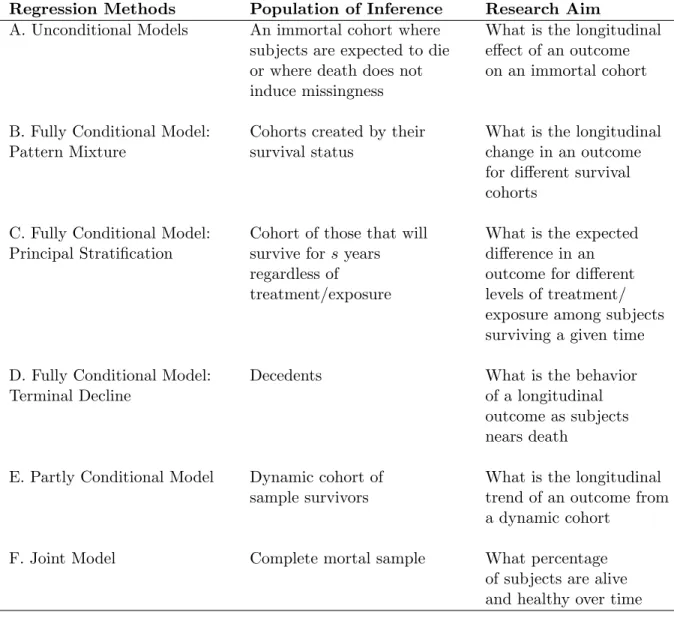
R. Allowing survival, S, to represent survival time such as age at death or weeks from baseline until death, the joint distribution f(yi,Si) denotes the probability that subject i’s outcomes takes a vector of specific values and survives to a specific time,s. In regression models that describe the relationship of predictors and the longitudinal outcomes, survival must be either implicitly or explicitly modeled. The joint probability can be factored in two ways: f(y)f(S|y) and f(y|S)f(S). Depending on how or if the longitudinal outcome conditions on survival status, S, the regression analysis of y can be categorized as being unconditional, fully conditional, partly conditional, or joint. When deciding which regression analysis should be considered for analysis of longitudinal data with follow-up truncated by death, Kurland et al. (2009) urged investigators to match analysis methods to research aims, for each method’s target population of inference are different for each model. Each method and its target population is summarized in Table 1.1 and described in the sections that follow.
1.4.2 Unconditional Models: f(yi)
if death does not affect the outcome. The estimation methods for these likelihood-based models implicitly impute values for those who die (Laird, 1988). Because of this fact, this method is typically not useful in gerontological research studies that are interested in the change of an outcome over time at the subject level. Yet, if the outcome of interest is focused on phenomena such as the rate of decline, recurrence, or other change following some action of a biological substance that can be collected at baseline and tested over time without requiring additional collections, then survival would not affect the outcome and the unconditional model would be a reasonable approach. Because unconditional models are assuming that death does not occur or that death does not cause truncation, the missing mechanism, survival, can be ignored without compromising the validity of the inference. This scenario follows a situation that is modeled by f(yi|Xi,β) =
R
Rifyi|Xi,β)dy m
i =f(yoi|Xi,β). 1.4.3 Fully Conditional Models: f(yi|Si =s)
Fully conditional mean models for y given S = s follow the pattern-mixture factorization of the joint distribution of (y, S),f(y,S) = f(y|S)f(S). In these models, inference regards the changing-over time of the longitudinal outcome variable stratified by the time of subjects’ deaths.
Pattern-Mixture
of death (Ribaudo et al., 2000; Pauler et al., 2003). Consequently, analysis will yield a mixture of distributions of the longitudinal response outcome. Each stratum will have its own trajectory of the response outcome. An advantage of this approach is accurate representation of individuals’ responses over time.
In order to better understand the nature of the proposed pattern-mixture models, let’s first examine the notation of the general pattern-mixture model as described by Little (1993). First, assume that there areq0, q1, . . . , qLmissing patterns in a population and let q0 represent the pattern with complete responses. Let ri take the value r for missing pattern qr, and let nr equal the number of subjects with qr missing pattern such that ΣL
r=0nr = N (total number of subjects). Now we have that ri follows a multinomial distribution with probability p(ri = r) = πr, r = 0,1, . . . , L. Finally, we can represent the distribution of yi as,
f(yi|ri,ϑ(r)) = f(y
(r)
i,o|ri =r,ϑ(or))f(y
(r)
i,m|ri =r,y
(r)
i,o,ϑ
(r)
m,r·o,r). (1.9)
yi,o(r) represent the observed responses in pattern qr and y
(r)
i,m represent the missing response variables in pattern qr. The parameters ϑ
(r)
o and ϑ(m,rr)·o,r are functions ofϑ(r) and are assumed to be distinct for all values ofr. Because death is a form of monotone missingness, the analysis within the patterns can ignore the non-response mechanism if separate analyses are conducted for each missing pattern.
Principal Stratification
pattern-mixture models, principal stratification not only conditions on actual survival, it also conditions on counterfactual survival status. The attractiveness of this method is that the inference is on the principal strata that would live regardless of exposure or treatment, allowing for the separation of the effect of the exposure and death from the effect of the exposure and the outcome. This approach is most useful in analyzing treatment and intervention effects in randomized clinical trials designs. However, this approach requires many untestable assumptions about the counterfactual information that is not collected.
The notation for principal stratification involves a vector of covariates, Xi, a manipulable exposure variable to which subjects can be randomized,Zi =z, a survival indicator for a subject at each exposure level, Di(z), such that Di(z) = 0 represents survival at exposure z, an indicator variable Ri for signifying if a subject reaches the end of the study, (Ri = 1 if not lost to follow-up; 0 otherwise), and the outcome for a subject at each exposure level,Yi(z). In this model, the interest lies in the estimate of the association of Zi and Yi(z) in the stratum of patients that will survive regardless of the value of z, Di(z) = 0 (alive) for all z, which can be assessed by estimating the unidentifiable survivor average causal effect (SACE), which is defined as
µ=E{Yi(1)|D(z) = 0]−E[Yi(0)|D(z) = 0}.
Terminal Decline
This fully conditional model is similar to the pattern-mixture model in that the missing pattern category determines the length of outcome vector. Unlike the pattern-mixture model, the terminal decline model allows the trajectory of the outcome over the new time scale to be estimated for the entire sample.
1.4.4 Partly Conditional Models: f(yi|Si > s)
Partly conditional models estimate the mean of the response conditioned on each subject being alive beyond time s. These models are different from the unconditional case where the analysis methods model the correlation structure of the repeated data implicitly and impute missing data without any differentiation between dropout due to death and dropout due to other reasons. In order to avoid this forced imputation, partly conditional models are estimated by treating longitudinal data as independent. Kurland and Heagerty (2005) call the partly conditional method “regression conditioning on being alive” (RCA). This method describes the dynamic cohort of survivors and models the change in the prevalence of the outcome among survivors at each measurement occasion.
As mentioned above, likelihood based approaches cannot directly estimate or parameterize partly conditional means; instead, the models are fit using generalized estimating equations (GEE) (Liang and Zeger, 1986) with independence working correlation. This analysis should yield consistent estimation as long as the model is correctly specified (Crowder, 1986).
1.4.5 Joint Models: f(yi,Si)
et al. (1995) introduced a joint model by defining the probability of being alive and healthy (PAH) and a related method to predict the PAH for a prescribed amount of time. Johnson (2002) models the PAH generally as
P AH(s) =P(Q(s)> q, S > s) = P(Q(s)> q|S > s)P(S > s), (1.10)
where S > S represents being alive at time s and Q(s) > q represents being healthy at times. Equation (1.10) has a very similar structure to the general pattern-mixture model and can be seen as a special case of the pattern-mixture model. However, unlike a pattern-mixture model that locks participants in specific strata, the PAH model allows subjects to move from being alive and healthy to being alive and unhealthy and vice versa. Subjects are not allowed to transition out of the dead strata once they have entered it.
1.5 Data: NC EPESE
illness prevention practices and to lengthen the time older adults can live independently in their own homes.
Funded by the National Institute on Aging (NIA), North Carolina Established Populations of Epidemiological Studies of the Elderly (NC EPESE), officially known as the Piedmont Health Survey of the Elderly, was the fourth site added to the larger multi-center prospective population-based epidemiologic study of health status and the physical, social, and cognitive functioning of persons 65 years of age and older living in communities. An additional major goal for the data collected at the North Carolina EPESE centers was to study racial difference in mortality and health of older persons. Established in 1986, the North Carolina cohort was a sample of 4,162 persons 65 years or older residing in households in Durham, Warren, Franklin, Granville, and Vance counties (one urban county, four rural) in the Central Piedmont area of North Carolina. The site was over 50% black and the geographic area selected was diverse, allowing both racial and urban/rural comparisons to be made regarding the distribution of certain risk factors and disease. Of the 4,162 subjects selected on the basis of a four-stage, race-stratified sampling design, 48% (including similar proportions of blacks and whites) lived in an urban setting. Participants were surveyed in person on four occasions: Wave 1 (1986-1987); Wave 2 (1989-1990); Wave 3 (1992-1993); and Wave 4 (1996-1997). At each of these waves, depression symptoms, blood pressure, and physical functioning level were among the outcomes that were measured.
et al. (1991) justified a CES-D score of 9 or more to be sufficient for categorizing those subjects who are pre-screened for being clinically depressed versus the 16 score cut-off established by Radloff (1977).
Blood pressure of all participants was measured by trained interviewers using the Hypertension Detection and Follow-Up Program protocol (1978). Participants were seated and a standard mercury column sphygmomanometer was employed. Two blood pressure measurements were taken. The outcome of interest for blood pressure for this dissertation was the average of these two measurements. We note here that nearly all the subjects were on a medication regiment to normalize blood pressure.
dependency. Combined, these three health responses represent different categories of the overall health, vitality, and independence of older adults.
1.6 Summary
Collecting longitudinal data on older populations leads to greater risks of truncation due to death. Analysis of changes in responses truncated by death is likely to be biased and thus survival should necessarily be considered in the analysis. The NC EPESE studies that were initiated by the National Institutes on Aging (NIA) to estimate the incidences and prevalences of health conditions and to uncover predictors and correlates of death and diseases should be analyzed with the most accurate techniques. Further, this study that followed the health of certain cohorts for 10 years could benefit from new techniques to incorporate death information when the interest is in the mean change over time of a morbidity outcome that is truncated by death.
In the literature there exist discussions and suggestions on incorporating missingness due to death in mean regression models. These models are assumed to be unbiased for the estimands and highlight the correct interpretation for each proposed model. Even though bias (onβ), estimation, and efficiency,V( ˆβ), are important components of data analysis, they have not been clearly reviewed and discussed for these models. In an attempt to provide guidelines for those analyzing gerontological longitudinal data in the presence of death, these components deserve attention and exploration.
Table 1.1: Summary of statistical regression models for longitudinal response and survival and its population of inference
Regression Methods Population of Inference Research Aim
A. Unconditional Models An immortal cohort where What is the longitudinal subjects are expected to die effect of an outcome or where death does not on an immortal cohort induce missingness
B. Fully Conditional Model: Cohorts created by their What is the longitudinal
Pattern Mixture survival status change in an outcome
for different survival cohorts
C. Fully Conditional Model: Cohort of those that will What is the expected Principal Stratification survive forsyears difference in an
regardless of outcome for different
treatment/exposure levels of treatment/ exposure among subjects surviving a given time
D. Fully Conditional Model: Decedents What is the behavior
Terminal Decline of a longitudinal
outcome as subjects nears death
E. Partly Conditional Model Dynamic cohort of What is the longitudinal
sample survivors trend of an outcome from
a dynamic cohort
F. Joint Model Complete mortal sample What percentage
CHAPTER 2: ANALYSIS OF NC EPESE TO INCORPORATE SURVIVAL IN THE ANALYSIS OF OUTCOMES
TRUNCATED DUE TO DEATH
2.1 Introduction
The North Carolina Established Populations of Epidemiological Studies of the Elderly (NC EPESE) was a prominent observational prospective study that has been utilized to provide the narrative of incidences and prevalences of chronic illness, cognitive and physical impairments, and other disabilities, along with their risk factors and the changes of these characteristics of older adults as they age in the community. Analyses of this study and its sister studies have informed the needs of health care services for the prevention of illnesses plaguing adults in later life and strategies for maintaining function of older adults aging outside of health care facilities. Since the end of 2012, there have been 341 publications in the form of manuscripts, letters, and books that referenced any of the EPESE studies. From 1996 to the end of 2012, there have been 90 publications on the NC EPESE, and only 6 of the publications used a form of longitudinal methodology for its primary statistical analysis. None of the 6 publications made any distinctions between missing not due to death and missing due to death.
strengths and weakness of each proposed method, an understanding of the role of death in conditions that affect physical function, quality of life, and self-sufficiency are incomplete. Incomplete knowledge of the proposed methods could lead to erroneous conclusions that could misinform important policy affecting the elderly.
2.2 Effect of Death in NC EPESE
but provided complete information up to their deaths.
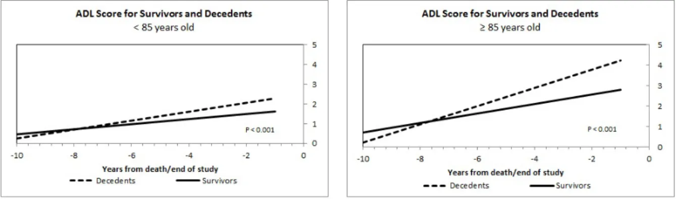
The effect of death in the modified NC EPESE was graphically assessed by dividing the decedents into two subgroups by baseline age–those greater than and equal to 85-years-old and those younger than 85. The population-expected means for the depression scores, the systolic and diastolic blood pressures, and the physical function scores up to 10 years prior to death were plotted. To serve as a reference, the end-of-study survivors were divided similarly into two subgroups and with their outcome trajectories graphed with their decedent counterparts.
In Figure 2.2, the decedents and survivors have similar mean CES-D scores 10 years from death (end of study). As the decedents approached death, their trajectories increased more sharply than the survivors’ trajectories in both cohorts. Although both trends increased over time, the trajectories were statistically different (p < 0.001) for those less than 85-years-old and those greater than or equal to 85.
The effect of death in Figure 2.3 for systolic blood pressure is not as apparent as in the depression data. Nonetheless, the systolic blood pressure trend for the survivors younger than 85 were nearly constant whereas the decedents experienced a decline. Both groups declined in the 85 and older graph and were not statistically different.
The population-expected mean diastolic blood pressure (Figure 2.4) for the survivors had a steeper decline over the 10-year period than the decedents in both age groups. The trends for the survivors and decedents were similar in each graph, albeit the trend for decedents 85-years-old and older was shifted down approximately two units.
Physical functional is known to be highly predictive of death. The results in Figure 2.5 supports this relationship. As decedents get closer to death, the number of ADLs accomplished alone decreased. If the decedents are older than 85, this trend is more severe.
difficult to correctly analyze and interpret findings without considering survival. The six regression models introduced by Kurland et al. (2009) are options for analyzing the outcomes with a treatment of survival.
2.3 Analysis of Modified NC EPESE
The unconditional, pattern-mixture models and terminal decline models (Kurland et al., 2009) for each outcome were fitted using a linear mixed model with a random intercept and slope as described by Laird and Ware (1982). The standard linear mixed effect model is written as
yi =Xiβ+Zidi+ei (2.1)
whereyi is a pi×1 of observations on person i for i= 1, . . . , N; Xi is a pi×q known, constant design matrix for personi;βis aq×1 vector of unknown, constant population parameters;Zi is api×2 known and constant design matrix for personi;di =
di0
di1
is the corresponding 2×1 vector of unknown random effects (random intercept and slope); and ei is a pi×1 vector of unknown random errors. Vectors di and ei are assumed to be from a Gaussian distribution and independent with meanE(di) =0 and E(ei) =0 and var(di) =D, where D =
σ2
d0 σd0d1
σd0d1 σ 2
d1
and var(ei) =Σei =σ
2I
i. Each model assumed homogenous variance for subjects measurements across time with no expected correlation between the measurements for all subjects,σ2I
i, (conditional on the random effects) and allowed the random effects to be independent with unique variances. Hence var(yi) =Vi =ZiDZiT +σ2Ii.
(1981b) may be used to obtain maximum likelihood estimates ofβ,di, D, and σ2. To see this, we take θ to the vector of the covariance components and then note that the estimates for the fixed and random effects when variance is unknown is given as
ˆ
β( ˆθ) =
N X
i=1
XiTWˆiXi
!−1 N X
i=1
XiTWˆiyi (2.2)
and
ˆ
d( ˆθ) = ˆDZiTWˆi(yi−Xiβˆ( ˆθ)). (2.3)
These are the weighted least square equations with estimates for ˆWi = ˆVi−1 with ˆ
Vi = ˆΣei+ZiDZˆ iT, where ˆΣei is the estimate of the variance-covariance matrix ofei. The variances of these estimates are defined as
ˆ
varhβˆ( ˆθ)i = N X
i=1
XiTWˆiXi
!−1
(2.4)
and
ˆ
varhdˆ( ˆθ)i = ˆDZiT
ˆ
Wi−WˆiXi
N X
i=1
XiTWˆiXi
!−1
XiTWˆi
ZiDˆ (2.5)
If di, ei, and yi were to be observed, then closed-forms of the maximum likelihood estimates of Σei and D based on quadratic forms in di and ei for i = 1, . . . , N can be obtained. For the variance structure assumed for the linear mixed models in this analysis (var(di) = Da 2×2 nonnegative definite matrix and thevar(ei) =Σei =σ2Ii)
these estimates would take the form
ˆ σ2 =
N X
i=1 eTi ei/
N X
i=1
pi =t1/
N X
i=1
and
ˆ
D =N−1
N X
i=1
didTi =t2/N. (2.7)
The equations above show that the sufficient statistics of the covariance components are t1 and the non-redundant components of the vector t2. An estimate of θ could
be used to approximate the estimates of the missing sufficient statistics by setting the sufficient statistics to their expectations given the observed outcome vector,yi. Before these equations can be denoted, we must define ˆθ, ˆβ( ˆθ) and ˆdi( ˆθ) to be estimates of
θ, β, anddi, respectively. Estimates of the sufficient statistics,t1 and t2 are computed
as
ˆ t1 =E
( N X
i=1
eTi ei|yi,βˆ( ˆθ),θˆ ) = N X i=1 n
EheTi ei|yi,βˆ( ˆθ),θˆ io = N X i=1 h ˆ
ei( ˆθ)Teˆi( ˆθ) + tr(var n
ei|yi,βˆ( ˆθ),θˆ o
)i
(2.8)
and
ˆ
t2 =E
( N X
i=1
didTi |yi,βˆ( ˆθ),θˆ ) = N X i=1 n E h
didTi |yi,βˆ( ˆθ),θˆ io = N X i=1 n ˆ
di( ˆθ) ˆdi( ˆθ)T +var
di|yi,βˆ( ˆθ),θˆ o
(2.9)
An alternative method for computing the ML estimates is the Newton-Raphson (N-R) algorithm for linear mixed-effects models, which are based on the first- and second-order partial derivatives of the log-likelihood functions. The log-likelihood of the stacked responses, yi, used to derive estimates is denoted as
l(y;β,θ) = −ln(2π) N X i=1 pi 2 − 1 2 N X i=1
ln|Vi| − 1 2
N X
i=1
(yi−Xiβ)TVi−1(yi−Xiβ). (2.10)
As detailed by Jennrich and Schluchter (1986), the N-R algorithm iteratively computes new parameter values from current parameter values, using
˜ β ˜ θ = β◦ θ◦ −
Hββ Hβθ
Hθβ Hθθ
−1
sβ sθ (2.11) with H =
Hββ Hβθ
Hθβ Hθθ
=
∂2l
∂β∂β
∂2l
∂β∂θ
∂2l
∂θ∂β
∂2l
∂θ∂θ
(2.12) and s= sβ sθ = ∂l ∂β ∂l ∂θ
. (2.13)
H is referred to as the Hessian matrix, andsis often described as the gradient or score vector. During the computation algorithm, these values are evaluated using the current values of the parameters.
appropriate option due to selection bias (Little and Rubin, 2002).
The pattern-mixture model, as denoted previously in equation 1.9, would average over all of the missing patterns, which would imply an implicit extrapolation within each pattern. This type of analysis is not useful when the missing patterns are due only to death. Therefore, Pauler et al. (2003) recommends considering death as a joint outcome instead of a nuisance parameter. Under this advice, the pattern-mixture model in the analysis of the modified NC EPESE is given as follows
yri =Xiβr+Zidri +e
r
i, (2.14)
where r represents the cohorts who died between the first follow-up and the second follow-up (r = 1), between the second follow-up and the third follow-up (r = 2), and the completers (r = 3). The covariance structures for pattern-mixture structures are the same used in the unconditional specifications for each cohort, r. This regression method is attractive because it should give accurate depictions of the trajectories of an outcome for each survival cohort, but requires conditioning on death, which is not known at baseline.
time from death. The structures of the covariance matrices remain unchanged from the unconditional and pattern-mixture models. Hence, the terminal decline model is modeled as
yi =Aiβ+Uidi+ei. (2.15)
The primary interest of the principal-stratification method is estimating the unidentifiable survivor average causal effect (SACE)(Frangakis and Rubin, 2002; Hayden et al., 2005; Holland, 1986; Robins and Greenland, 2000; Rubin, 1974, 2000), which is defined as the difference in the outcome for those with the exposure or treatment and the outcome of those without the exposure given participants would survive despite their assigned exposure group. Using the notation introduced in Chapter 1, the SACE takes the following form for a continuous outcome
µ∗ =E[Yi(1)|D(z) = 0]−E[Yi(0)|D(z) = 0]. (2.16)
Although others have proposed estimation methods for the SACE for randomized studies (Gilbert et al., 2003; Hayden et al., 2005; Zhang and Rubin, 2003), the SACE in this dissertation uses the estimation method proposed by Egleston et al. (2007). This estimation method was developed to be used in observational studies and estimates the SACE by using a set of unidentifiable assumptions. This estimation was designed to correct the bias that may be a result of both non-response and baseline differences for those with or without the exposure. To describe the estimation method, the notation present in Chapter 1 must be revisited.
denoted by D(Z), such that D(Z) = 0 represents survival for exposure status Z. An indicator variable R signifies if a subject reaches the end of the study, (R = 1 if not lost to follow; 0 otherwise), and the outcome for exposure is given as Y(Z). For each exposure value,n independent and identically distributed observed data were gathered,
O ={Oi ={Xi, Zi, Di, Ri( if Di = 0), Yi( if Di = 0 andRi = 1)}, i= 1, . . . , n}.
The four principal strata are defined as
1. Individuals who would survive regardless of exposure, D(0) =D(1) = 0. (S1)
2. Those who would die if they have the exposure but survive if they do not, D(0) = 0, D(1) = 1. (S2)
3. Those who would die regardless of exposure, D(0) =D(1) = 1. (S3)
4. Those who would die if they do not have the exposure of interest and would survive if they do, D(0) = 1, D(1) = 0. (S4)
The assumptions evoked to identify SACE are given below.
1. Stable Unit Treatment Value Assumption (Rubin, 1980), which states that individual’s potential outcomes are not dependent on the exposure status of either the other participants potential outcomes or the mechanism in which the exposure was acquired.
is not allowed in this estimation. This assumption may be violated for some of the exposure levels for evidence exists of gender-race death associations (Yao and Robert, 2011).
3. Strong ignorability of “treatment” assignment (Rosenbaum and Rubin, 1983) implies that developing an exposure is independent of the potential outcomes given the covariates. In an observational study, this assumption means that the exposure statuses (exposed vs. not exposed) are similar within each covariate level. Thus, the probability of an individual surviving given membership or non-membership in the exposure group given the covariates is denoted as gz(X) = P[D(Z) = 0|X]. Further E[Y(Z)|D(Z) = 0,X] =E[Y|D= 0, Z =z,X].
4. For those who survive, the non-response of the non-mortality outcome is independent of the value of the outcomes within levels of exposure status and covariates. This provides a situation that is similar to the missing at random (MAR) assumption. Coupled with the previous assumption, this assumption makes it possible to identify the expected mean of the outcome for those who would survive but have missing outcomes within the exposure status and covariates. That is, hz(X) = E[Y(Z)|D(Z) = 0,X].
The quantity displayed in the results section is the estimate to E[Y(1)|D(Z) = 0, R= 1,X] at each survey follow-up period. From the above assumptions, we have the following:
E[Y(1)|S1] = E[Y(1)|D(1) = 0] =E{E[Y(1)|D(1),X]}
The mean for each race-gender “exposure” was estimated for each measurement occasion using ordinary least squares regression (h1(X)) and the g1(X) was estimated
from a logistic regression model. Only one covariate, baseline age centered about the mean, was considered for both models.
The trends produced by the partly conditional model estimate the expected population mean trend on the subject being alive. This method is useful when the interest is the regression of a repeated measure on the participant being alive. That is, E(Yij|Xij, Si > tj). Likelihood methods like the linear mixed model discussed above do not directly parameterize partly conditional models for the estimation method imposes responses for decedents. Rather, Kurland and Heagerty (2005) demonstrate that the generalized estimating equations (Liang and Zeger, 1986) with an independent working correlation directly parameterize the regression model for the target population of those who are alive at the time of collection.
For the partly conditional mean µU
ij = E(Yij|Xij), an unbiased, linear quasi-score equation for the regression parameter vectorβU is given by
U(βU) = N X
i=1
pi X
j=1
∂µU ij
∂β (Yij −µ U
ij). (2.17)
By letting Aij be an indicator variable that equals 1 if Si > tj and 0 otherwise, the quasi-score contributions can be restricted to ensure inference on the target population. The new quasi-score equation becomes
U(βA) = N X
i=1
pi X
j=1
Aij ∂µA
ij
∂βA(Yij −µ A
ij). (2.18)
parameterized partly conditional regression model with a link functiong.
g(µAi ) =XiβA, (2.19)
where µAij = E(yij|Xij, Si > tj) = E(yij|Xij, Aij = 1) given that the regression model is correctly specified (Crowder, 1986). The outcomes for this model were fitted as a generalized linear regression model with an identity link and an independent working correlation structure.
The probability of being alive and healthy (PAH) (Johnson, 2002) for each participant i was calculated according to the following equation:
P AH(s)i =P(Qi(s)> q,Si > s|Xi) = P(Qi(s)> q|Si > s)P(Si > s), (2.20)
where Q(s)i represents the dichotomous health variable and Si represent the survival time variable. Utilizing repeated logistic regression with an unstructured correlation matrix, the probability of being not depressed (< 9 depressive symptoms), the probability of being non-hypertensive (systolic blood pressure<140 or diastolic blood pressure<90), and the probability of not having any activities of daily living limitations (ADL<1) were calculated for each follow-up period and each gender-race combination. The probability of survival was estimated from a Cox proportional hazards model given by
λ(s|x) = λ0(s) exp(β1x1+β2x2+. . .+βpxp) = exp(β0x), (2.21)
likelihood models would produce unbiased estimates. In contrast, missingness that is not missing at random (NMAR) could introduce bias in the estimation.
2.4 Results
Figure 2.6(a)-(f), Figure 2.7(a)-(f), Figure 2.8(a)-(e) and Figure 2.9(a)-(f) depict the results of the analysis of the Duke EPESE data using the different proposed methods for assessing the rates of change based on research inquiries for depression scores (CES-D), systolic blood pressure, diastolic blood pressure, and physical function (ADLs), respectively. In all of the models, the baseline variables–age (centered about the mean), race (1 if subjects identify as black and 0 if subjects identify as white), and gender (1 if subjects are identified as male and 0 if subjects are identified as female) – are included as covariates with the exception of the principal stratification model. The principal stratification model uses one’s race and gender identification as exposures and age as the only covariate.
2.6(d)), women had about four depressive symptoms, which is approximately one more than their male counterparts. The terminal decline trends were similar by race. The dynamic cohort’s depression rates of change, as modeled by the partly conditional model, were two units lower than those reported in the model assuming an immortal cohort (unconditional model), but the trends were similar. Although men began the study with a higher probability of being alive and having less than nine depressive symptoms (0.92 vs. 0.89; Figure 2.6(f)), over time women became more likely to be healthy and alive.
men were approximately 50% alive and non-hypertensive. As the groups aged, the men’s probability of being alive and non-hypertensive declined more rapidly than the women’s rates.
Rates of change in the mean diastolic blood pressure for the immortal cohort were similar across race-gender groups. Additionally, black women and men had similar baseline values for diastolic blood pressure measurements, which remained true for white men and women (Figure 2.8(a)). In Figure 2.8(b), the baseline values of diastolic blood pressure are very similar across the survival cohorts for each race-gender group. Nonetheless, white men and women who died after the first follow-up only experienced small declines in their diastolic blood pressure measurements annually. The trend of diastolic blood pressure for those who would survive regardless of race or gender had similar baseline values to the unconditional and pattern-mixture completers’ regression models, except for white males. Although the baseline values are similar, the rates of change for the principal stratification were much higher than the other two methods. Men’s mean diastolic blood pressure declined more rapidly than the womens as they neared death (Figure 2.8(d)). Figure 2.8(e) displays the estimated means of diastolic blood pressure for those alive at the given follow-up occasion. These values are similar to the unconditional model results.
women approach death, their physical function dependency increased more rapidly than men (0.30 versus 0.25). The physical functioning estimated means of the mutable population had comparable means to the mean estimates of the unconditional model for each race-gender group (Figure 2.9(e)). Black women were the most physically limited at baseline with a PAH of 0.63. The others had probabilities greater than 0.70. Even though the annual rate of decline was slightly higher for males than females (0.07 annual rate of decline), the graphical trends were alike.
2.5 Simulation of Varying Death Burden
To evaluate the ability of the unconditional, pattern-mixture, and partly conditional models to estimate rates of change in the Center for Epidemiologic Studies Depression (CES-D) scores, systolic and diastolic blood pressures, and activities of daily living (ADL) of a complete dataset without bias for various MCAR burdens of death, we simulated a sample from a theoretical population. Each of the four outcomes were treated as continuous outcomes and were generated from the mixed model with a random intercept and slope as described in equation (2.1). Four waves of longitudinal outcomes were simulated from a normal distribution with mean Xiβ and covariance
were generated accordingly: white males (π= 0.16), black males (π = 0.19), and white females (π = 0.29). Age was simulated assuming it was from a normal distribution dictated by the mean and standard deviation in each race-gender group from the NC EPESE. Similarly, time of measurements mirrored the NC EPESE. Thus, we assume measurements were only possible at baseline, and 3, 6, and 10 years post-baseline. The values of the parametersβ, σ2,andDused in the simulation are given for each outcome
below.
CES-D score: βT =
3.243 0.086 0.065 0.356 −0.686 0.001 0.003
Σi =Zi
5.32 −0.14 −0.14 0.39
Z
T
i + 7.16Ii
Systolic BP: βT =
143.29 0.088 0.002 0.756 −2.326 −0.017 −0.136
Σi =Zi
139.69 −3.38 −3.38 0.91
Z
T
Diastolic BP: βT =
77.258 0.799 −0.289 2.775 1.529−0.0006−0.010
Σi =Zi
47.66 −2.26 −2.26 0.39
Z
T
i + 92.94Ii
ADL score: βT =
0.742 0.211 0.114 0.243 0.133 0.001 −0.063
Σi =Z
1.52 −0.002 −0.002 0.04
Z
T + 1.78I i
2.6 Simulations Results
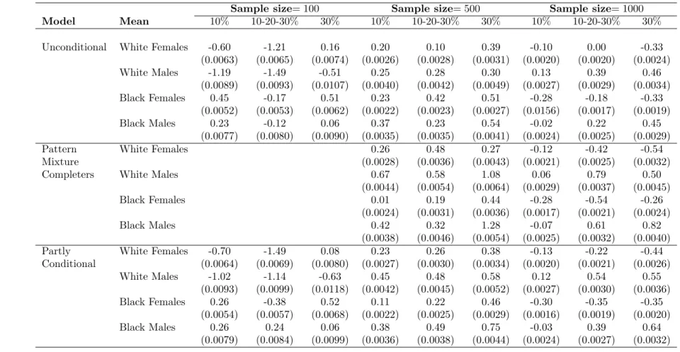
The choice is made to fit the unconditional, pattern-mixture, and partly conditional models as described earlier for each of the 1,000 samples and for the three death percentage scenarios. All analyses were performed using SAS v9.2. For the unconditional and pattern-mixture models, maximum likelihood estimation was provoked. The partly conditional models were estimated by generalized estimating equations using an identity working correlation matrix and empirical standard errors to account for the repeated continuous measures per subject. The relative bias of the estimation for each mean per racegender combination was computed. Tables 2.1 -2.4 give the mean bias for each method by the different death percentage scenario. Pattern-mixture models could only be performed for the 500 and 1,000 sample sizes. The sample size ofN = 100 did not provide enough participants for the survival cohorts for some of the missing schemes.
because this groups estimation depends on the estimation of all parameters.
2.7 Discussion
By considering survival in the estimation of depression, systolic and diastolic blood pressures, and functional dependency over time, the analyses presented in this paper contribute to the previous understanding of the nature of these outcome through a new level of reliability of the estimates as well as depictions of the outcomes trajectories. Because the NC EPESE was part of an inaugural study on older adults living in America and the only dataset that allowed for adequate race comparison, the dataset has been studied intensely, in particular, for the outcome of depression. Blazer et al. (1991) examined the association of age and depression using a cross-sectional regression analysis. Their analysis concluded that age and depression had an indirect relationship when adjusted for gender, income, physical disability, cognitive impairment, and social support. Although our analysis did not account for some of the key covariates associated with depression, each of the six models supported a direct association of aging and depression, except for the trend for those black males who died before the second follow-up. Furthermore, the graphs presented in 2.6(a)-(f) offer one of the few longitudinal trends of depression on the North Carolina Established Populations of Epidemiological Studies of the Elderly (NC EPESE). Thus, these results contributes to what we know about depression over time for older adults.
that when survival status and hypertension are modeled together, a gender association is more prominent than a race association. The joint model supports similar results by gender in terms of both baseline values and rates of change in the probability of being alive and healthy over time. However, race associations with blood pressure are visible in the analysis of diastolic blood pressure.
Currently, mobile disability is defined as difficulty or dependency in carrying out activities essential to independent living and desired activities important to ones quality of life; it is typically screened through Activities of Daily Living (ADL) and Instrumental Activities of Daily Living (IADL) citeptopinkova. Although this study utilized only the ADL score to define limitations of physical functioning, the previously reported racial gap in disability remained supported citeptaylor.
The major contribution of this study was the use of advanced statistical methods that included survival status in the estimation of the longitudinal means of outcomes from a subpopulation (NC EPESE) of the popular longitudinal study of older adults. Additionally, the appropriate populations and aims of these models were presented. These current findings, along with previous results of these outcomes, strengthen the understanding of accurate changes of the outcome measures as a cohort of older adults become older.
was lower. The relative biases of the estimates of the mean of activities of daily living scores were notably larger than the other outcomes, especially for black males. The mean estimates for black males were dependent on all of the parameter estimates. The reason for this occurrence is not quite clear, but we suspect that there may exist a vulnerability in our simulation used to generate the data. With the exception of the results from ADL, the models seem to perform quite well when the missing assumption is MCAR.
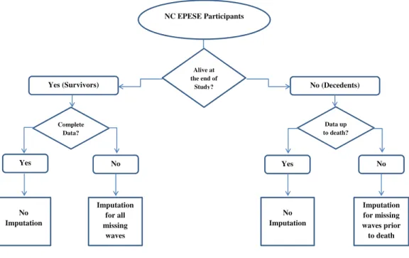
Figure 2.1: Data imputation decision chart.
NC EPESE Participants
Alive at the end of
Study?
Yes (Survivors) No (Decedents)
Complete Data?
Data up to death?
Yes No Yes No
No Imputation
Imputation for all missing waves
No Imputation
Imputation for missing waves prior to death
Figure 2.2: Mean Depression Score for those >85 and those≥85 years old.
Thepvalue in each panel corresponds to the test of the difference in the rate of change due to death.
Figure 2.3: Mean Systolic Blood Pressure for those >85 and those≥85 years old.
Thepvalue in each panel corresponds to the test of the difference in the rate of change due to death.
Figure 2.4: Mean Diastolic Blood Pressure for those >85 and those≥85 years old.
Figure 2.5: Mean Functional Score for those>85 and those≥85 years old.
Figure 2.6: Fitted trajectories of CES-D scores for EPESE participants
a) Unconditional
c) Fully Conditional: Principal Stratification
e) Partly Conditional
b) Fully Conditional: Pattern-Mixture
d) Fully Conditional: Terminal Decline
f) Joint Model
0 1 2 3 4 5
0 1 2 3 4 5 6 7 8 9 10
C E S -D S co re
Years post baseline Depression: Unconditional Model
Black Female White Female Black Male White Male 0 1 2 3 4 5
0 1 2 3 4 5 6 7 8 9 10
C E S -D S co re
Years post baseline
Depression: Principal Stratification Model
Black Female White Female Black Male White Male 0 1 2 3 4 5
0 1 2 3 4 5 6 7 8 9 10
C E S -D S co re
Year post baseline Depression: Partly Conditional Model
Black Female White Female Black Male White Male 0 1 2 3 4 5
0 1 2 3 4 5 6 7 8 9 10
C E S -D S co re
Year post baseline Depression: Pattern Mixture Model
Black Female White Female Black Male White Male 0 1 2 3 4 5
-10 -9 -8 -7 -6 -5 -4 -3 -2 -1 0
C E S -D S co re
Year from death Depression: Terminal Decline Model
Black Female White Female Black Male White Male 0 0.1 0.2 0.3 0.4 0.5 0.6 0.7 0.8 0.9 1
0 1 2 3 4 5 6 7 8 9 10
P
A
H
Years post baseline Depression and Survival: Joint Model
Figure 2.7: Fitted trajectories of systolic blood pressure for EPESE participants
a) Unconditional
c) Fully Conditional: Principal Stratification
e) Partly Conditional
b) Fully Conditional: Pattern-Mixture
d) Fully Conditional: Terminal Decline
f) Joint Model
130 135 140 145 150 155 160
0 1 2 3 4 5 6 7 8 9 10
m
m
H
g
Years post baseline
Systolic BP: Unconditional Model
Black Female White Female Black Male White Male 130 135 140 145 150 155 160
0 1 2 3 4 5 6 7 8 9 10
m
m
H
g
Years post baseline
Systolic BP: Prinicpal Stratification Model
Black Female White Female Black Male White Male 130 135 140 145 150 155 160
0 1 2 3 4 5 6 7 8 9 10
m
m
H
g
Years post baseline
Systolic BP: Partly Conditional Model
Black Female White Female Black Male White Male 130 135 140 145 150 155 160
0 1 2 3 4 5 6 7 8 9 10
m
m
H
g
Years post baseline
Systolic BP: Pattern Mixture Model
Black Female White Female Black Male White Male 130 135 140 145 150 155 160
-10 -9 -8 -7 -6 -5 -4 -3 -2 -1 0
m
m
H
g
Years to death
Systolic BP: Terminal Decline
Black Female White Female Black Male White Male 0 0.1 0.2 0.3 0.4 0.5 0.6 0.7 0.8 0.9
0 1 2 3 4 5 6 7 8 9 10
P
A
H
Years post baseline
Normal Blood Pressure and Survival: Joint Model
Figure 2.8: Fitted trajectories of diastolic blood pressure for EPESE participants
a) Unconditional
c) Fully Conditional: Principal Stratification
e) Partly Conditional
b) Fully Conditional: Pattern-Mixture
d) Fully Conditional: Terminal Decline
60 65 70 75 80 85 90
0 1 2 3 4 5 6 7 8 9 10
m
m
H
g
Years post baseline
Diastolic BP: Unconditional Model
Black Female White Female Black Male White Male 60 65 70 75 80 85 90
0 1 2 3 4 5 6 7 8 9 10
m
m
H
g
Years post baseline
Diastolic BP: Prinicpal Stratification Model
Black Female White Female Black Male White Male 60 65 70 75 80 85 90
0 1 2 3 4 5 6 7 8 9 10
m
m
H
g
Years post baseline
Diastolic BP: Partly Conditional Model
Black Female White Female Black Male White Male 60 65 70 75 80 85 90
0 1 2 3 4 5 6 7 8 9 10
m
m
H
g
Years post baseline
Diastolic BP: Pattern Mixture Model
Black Female White Female Black Male White Male 60 65 70 75 80 85 90
-10 -9 -8 -7 -6 -5 -4 -3 -2 -1 0
m
m
H
g
Years to death
Diastolic BP: Terminal Decline
Figure 2.9: Fitted trajectories of ADL Scores for EPESE participants
a) Unconditional
c) Fully Conditional: Principal Stratification
e) Partly Conditional
b) Fully Conditional: Pattern-Mixture
d) Fully Conditional: Terminal Decline
f) Joint Model
0 1 2 3 4 5
0 1 2 3 4 5 6 7 8 9 10
A D L S co re
Years post baseline ADL: Unconditional Model
Black Female White Female Black Male White Male 0 1 2 3 4 5
0 1 2 3 4 5 6 7 8 9 10
A D L S co re
Years post baseline ADL: Principal Stratification Model
Black Female White Female Black Male White Male 0 1 2 3 4 5
0 1 2 3 4 5 6 7 8 9 10
A D L S co re
Years from baseline ADL: Partly Conditional Model
Black Female White Female Black Male White Male 0 1 2 3 4 5
0 1 2 3 4 5 6 7 8 9 10
A D L S co re
Years post baseline ADL: Pattern Mixture Model
Black Female White Female Black Male White Male 0 1 2 3 4 5
-10 -9 -8 -7 -6 -5 -4 -3 -2 -1 0
A D L S co re
Years from death ADL: Terminal Decline Model
Black Female White Female Black Male White Male 0 0.1 0.2 0.3 0.4 0.5 0.6 0.7 0.8 0.9 1
0 1 2 3 4 5 6 7 8 9 10
P
A
H
Years from baseline ADL: Joint Model
Table 2.1: CES-D - Relative Bias (×100) and (SE) of mean estimates five years post-baseline based on 1000 simulated samples with three follow-up times at varying percentages of death per wave
Sample size= 100 Sample size= 500 Sample size= 1000
Model Mean 10% 10-20-30% 30% 10% 10-20-30% 30% 10% 10-20-30% 30%
Unconditional White Females -0.60 -1.21 0.16 0.20 0.10 0.39 -0.10 0.00 -0.33
(0.0063) (0.0065) (0.0074) (0.0026) (0.0028) (0.0031) (0.0020) (0.0020) (0.0024)
White Males -1.19 -1.49 -0.51 0.25 0.28 0.30 0.13 0.39 0.46
(0.0089) (0.0093) (0.0107) (0.0040) (0.0042) (0.0049) (0.0027) (0.0029) (0.0034)
Black Females 0.45 -0.17 0.51 0.23 0.42 0.51 -0.28 -0.18 -0.33
(0.0052) (0.0053) (0.0062) (0.0022) (0.0023) (0.0027) (0.0156) (0.0017) (0.0019)
Black Males 0.23 -0.12 0.06 0.37 0.23 0.54 -0.02 0.22 0.45
(0.0077) (0.0080) (0.0090) (0.0035) (0.0035) (0.0041) (0.0024) (0.0025) (0.0029)
Pattern White Females 0.26 0.48 0.27 -0.12 -0.42 -0.54
Mixture (0.0028) (0.0036) (0.0043) (0.0021) (0.0025) (0.0032)
Completers White Males 0.67 0.58 1.08 0.06 0.79 0.50
(0.0044) (0.0054) (0.0064) (0.0029) (0.0037) (0.0045)
Black Females 0.01 0.19 0.44 -0.28 -0.54 -0.26
(0.0024) (0.0031) (0.0036) (0.0017) (0.0021) (0.0024)
Black Males 0.42 0.32 1.28 -0.07 0.61 0.82
(0.0038) (0.0046) (0.0054) (0.0025) (0.0032) (0.0040)
Partly White Females -0.70 -1.49 0.08 0.23 0.26 0.38 -0.13 -0.22 -0.44
Conditional (0.0064) (0.0069) (0.0080) (0.0027) (0.0030) (0.0034) (0.0020) (0.0021) (0.0026)
White Males -1.02 -1.14 -0.63 0.45 0.48 0.58 0.12 0.54 0.55
(0.0093) (0.0099) (0.0118) (0.0042) (0.0045) (0.0052) (0.0027) (0.0030) (0.0036)
Black Females 0.26 -0.38 0.52 0.11 0.22 0.46 -0.30 -0.35 -0.35
(0.0054) (0.0057) (0.0068) (0.0022) (0.0025) (0.0029) (0.0016) (0.0019) (0.0020)
Black Males 0.26 0.24 0.06 0.38 0.49 0.75 -0.03 0.39 0.64
(0.0079) (0.0084) (0.0099) (0.0036) (0.0038) (0.0044) (0.0024) (0.0027) (0.0032)