Robustness of stepwise latent class modeling with continuous distal outcomes

(1)

Full Terms & Conditions of access and use can be found at

http://www.tandfonline.com/action/journalInformation?journalCode=hsem20

Download by: [Universiteit Leiden / LUMC] Date: 17 November 2015, At: 04:40

Structural Equation Modeling: A Multidisciplinary Journal

ISSN: 1070-5511 (Print) 1532-8007 (Online) Journal homepage: http://www.tandfonline.com/loi/hsem20

Robustness of Stepwise Latent Class Modeling

With Continuous Distal Outcomes

Zsuzsa Bakk & Jeroen K. Vermunt

To cite this article: Zsuzsa Bakk & Jeroen K. Vermunt (2015): Robustness of Stepwise Latent Class Modeling With Continuous Distal Outcomes, Structural Equation Modeling: A Multidisciplinary Journal, DOI: 10.1080/10705511.2014.955104

To link to this article: http://dx.doi.org/10.1080/10705511.2014.955104

Published online: 15 May 2015.

Submit your article to this journal

Article views: 88

View related articles

View Crossmark data

(2)

Robustness of Stepwise Latent Class Modeling With

Continuous Distal Outcomes

Zsuzsa Bakk and Jeroen K. Vermunt

Tilburg University

Recently, several bias-adjusted stepwise approaches to latent class modeling with continuous distal outcomes have been proposed in the literature and implemented in generally available software for latent class analysis. In this article, we investigate the robustness of these meth-ods to violations of underlying model assumptions by means of a simulation study. Although each of the 4 investigated methods yields unbiased estimates of the class-specific means of distal outcomes when the underlying assumptions hold, 3 of the methods could fail to different degrees when assumptions are violated. Based on our study, we provide recommendations on which method to use under what circumstances. The differences between the various stepwise latent class approaches are illustrated by means of a real data application on outcomes related to recidivism for clusters of juvenile offenders.

Keywords: latent class analysis, robustness, stepwise approaches

Latent class (LC) analysis is a method widely used in the social and behavioral sciences to group individuals based on their responses on a set of observed variables (Goodman,

1974). Examples include the creation of a clustering concerning tolerance toward nonconformity (McCutcheon,

1985) or a typology of psychological contract types (De Cuyper, Rigotti, Witte, & Mohr,2008). Often in LC anal-ysis applications the interest lies not only in obtaining a clustering, but also in determining whether the classes dif-fer with respect to one or more, possibly continuous, distal outcome variables. For example, De Cuyper et al. (2008) tested whether the means of variables related to well-being differed for latent classes representing types of psycho-logical contracts; Pastor, Barron, Miller, and Davis (2007) studied differences in academic achievement of college stu-dents across goal orientation clusters; and Mulder, Vermunt, Brand, Bullens, and Van Merle (2012) compared the means of 70 variables measuring different aspects of recidivism across clusters of juvenile offenders.

The class-specific means of a distal outcome can be deter-mined by either a one-step or a stepwise approach. In the

Correspondence should be addressed to Zsuzsa Bakk, Methodology and Statistics, Tilburg University, Warandelaan 2, Tilburg, 5037AB, The Netherlands. E-mail:[email protected]

one-step approach, the distal outcome is incorporated in the LC model as an additional response variable and the resulting expanded model is estimated in the usual way. This approach has several disadvantages, however. The main problem is related to the fact that rather strong assumptions need to be made about the within-class distribution of the distal outcome, and if these assumptions are violated the original LC model could be completely distorted. A related issue is that it is problematic to deal with multiple distal outcomes, which could either be dealt with simultaneously, requiring strong assumptions about their joint distribution, or one by one, implying that the LC solution might change per distal outcome. Furthermore, because the interest lies in explaining differences across classes in the distal outcome, using the distal outcome as one of the variables defining the latent classes creates an unintended circularity. Because of these problems, researchers often prefer using a three-step approach in which one first builds the LC model without the distal outcome(s), then determines the class memberships, and subsequently investigates the relationship between class memberships and the distal outcome(s), say using a sim-ple analysis of variance (ANOVA; Bakk, Tekle, &; Vermunt,

2013). However, a well-known disadvantage of this approach is that the estimates obtained in the third step are attenuated because of the classification error introduced when assigning individuals to classes (Bolck, Croon, & Hagenaars,2004).

(3)

Recently, alternative three-step approaches have been pro-posed that yield unbiased estimates of the class differences in the distal outcome (Bakk et al., 2013). One method, called ML involves estimating the class-specific means and variances by maximum likelihood while correcting for the classification errors (Bakk et al., 2013; Vermunt, 2010). Another approach based on the work of Bolck et al. (2004), which we therefore call the BCH approach, involves per-forming a weighted ANOVA, with weights that are inversely related to the classification error probabilities (Bakk et al.,

2013; Vermunt, 2010). Both approaches can be used with either equal or unequal variance across classes.

A different type of stepwise approach for dealing with dis-tal outcomes was proposed by Lanza, Tan, and Bray (2013). This approach, which we refer to as the LTB approach, involves estimating an LC model in which the distal outcome of interest is used as a covariate predicting class mem-bership using a logistic model rather than as a response variable affected by the classes. As a second step, the class-specific means for the distal outcome are calculated from the parameters of the estimated LC model using Bayes theorem. Although simulation studies have shown that these three recently developed stepwise approaches (ML, BCH, and LTB) yield unbiased estimates of the class-specific means of distal outcomes when all underlying model assumptions hold (Bakk et al.,2013; Lanza et al.,2013), it is unknown whether these methods are robust for violations of these assump-tions. For example, the ML and BCH approaches assume that the distal outcome is normally distributed within classes. whereas the ML approach is expected to be affected by viola-tions of this assumption (Asparouhov & Muthén,2014), the BCH approach is probably more robust because it is simi-lar to a standard ANOVA. At the same time, for continuous variables, the LTB approach assumes that the relationship between the latent classes and the distal outcome is linear on a logit scale, and it is unknown whether violation of this assumption will bias the estimates of the class-specific means. In the remainder of this article, we first introduce the different types of stepwise approaches and describe their assumptions. Subsequently, in a simulation study, we com-pare the performance of the various approaches when certain underlying assumptions are violated. Next, we illustrate the methods with an analysis of a data example on juvenile recidivism. We end with a discussion and recommendations regarding the use of the different methods.

THE BASIC LATENT CLASS MODEL AND APPROACHES FOR DEALING WITH A

CONTINUOUG DISTAL OUTCOME

In the following, we first introduce the basic LC model. Then, we describe different ways to deal with distal out-comes; that is, the simultaneous or one-step method, the LTB approach, and the three-step ML and BCH approaches.

Special attention is dedicated to the assumptions made by the various approaches.

The Basic LC Model and Its Extension to Include a Continuous Distal Outcome

LetYikdenote the response of individualion one ofK

cat-egorical response variables, where 1≤k≤K and 1≤i≤ N. The full response vector is denoted byYi. LC analysis

assumes that individuals belong to one of theT categories of an underlying categorical latent variableXthat affects the responses (Goodman,1974; Hagenaars,1990; McCutcheon,

1987). Denoting a particular latent class byt,the model can be formulated as follows:

P(Yi)= T

t₌1

P(X=t)P(Yi|X=t), (1)

whereP(X=t)represents the (unconditional) probability of belonging to classt andP(Yi|X=t)represents the

class-specific distribution of the responsesYi. These class-specific

distributions are simplified further by assuming that the K response variables are independent within classes, which is known as the local independence assumption. This yields:

P(Yi)= T

t₌1

P(X=t)

K

k₌1

P(Yik|X=t). (2)

For categorical responses, P(Yik|X=t)= Rk

r₌1

πI₍Yik=r),

ktr

whereπktris the probability of giving responseron variable

kfor classt,andI(Yik=r)is an indicator variable taking on

the value 1 ifYik=rand 0 otherwise.

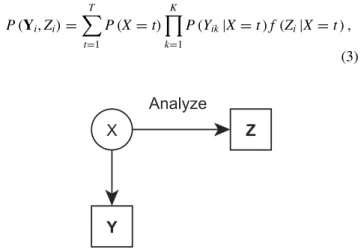
The basic LC model described in Equation 2 can be extended to include a continuous distal outcome denoted by Zi (visualized inFigure 1). This yields the following joint

model forYiandZi.

P(Yi,Zi)= T

t₌1

P(X=t)

K

k₌1

P(Yik|X=t)f(Zi|X=t),

(3)

FIGURE 1 One-step approach.

(4)

wheref(Zi|X=t)denotes the class-specific distribution of

Zi, which for continuous distal outcomes is typically defined

to be a normal distribution with meanμt and varianceσt2.

Note that the distal outcome serves as an additional response variable in the LC model.

The main disadvantage of this simultaneous modeling procedure is that the inclusion of Z in the model can alter the meaning of the classes (Petras & Masyn,2010), especially when the normal distribution assumption for f(Zi|X=t)does not hold. Such a misspecification can even

lead to overextraction of the classes (Bauer & Curran,2003). Moreover, when respecifying the model for a different out-come variable, the definition of the classes could change. Another disadvantage is that from a substantive perspec-tive it is undesired that the distal outcome contributes to the definition of the classes; that is, it creates a kind of circu-larity. To prevent these problems, alternative methods were proposed that we present in the following.

The LTB Approach

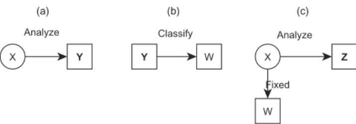
To overcome the problems of the one-step approach result-ing from the normal distribution assumption for Z, Lanza et al. (2013) proposed an alternative procedure that does not require making such an assumption. The LTB approach is a two-step procedure, that proceeds as follows:

1. Estimate an LC model in which Z is included as a covariate instead of a response variable (Figure 2a). 2. Based on the estimates from the first step, calculate the

class-specific means forZ(Figure 2b).

In the first step, “covariate”Z is added to the model by extending the basic LC model described in Equation 2 as follows:

P(Yi|Zi)= T

t=1

P(X=t|Zi) K

k=1

P(Yik|X=t), (4)

whereP(X=t|Zi) denotes the probability of belong to class

tgiven the “covariate” valueZi.This probability is modeled

by a multinomial logistic regression equation; that is,

(b) (a)

FIGURE 2 The two steps of the LTB approach.

P(X=t|Zi)=

eαt+βtZi

T

s=1

eαs+βsZi

, (5)

with interceptsαtand slopesβt.

The second step involves computing the class-specific meansμt. It should be noted that these can be obtained as

follows:

μt=

Z

f(Z|X=t) (6)

where f(Z|X=t), the class-specific distribution of Z, can be calculated using Bayes theorem as follows (Lanza et al.,

2013):

f(Z|X=t)=f(Z)P(X=t|Z)

P(X=t) . (7)

The quantities P(X=t|Z) and P(X=t) can be obtained from the estimated LC model, butf(Z) is unknown. Lanza et al. (2013) suggested approximatingf(Z) by a kernel den-sity estimate, and calculate the class-specific mean ofZusing this estimate.

However, as suggested by Asparouhov and Muthén (2014), a much simpler solution is to use the empirical distribution of Z, which involves replacing the integral in Equation 6 by a sum over theNsample units and replacing f(Z) in Equation 7 by _N1. This yields:

μt= N

i₌1

Zi

P(X=t|Zi)

N P(X=t). (8)

This is how the LTB method is implemented in Mplus 7.1 (Muthén & Muthén, 1998–2012) and LatentGOLD 5.0 (Vermunt & Magidson,2013).

Lanza et al. (2013) did not discuss standard error (SE) estimation for theμt, implying that they did not solve the

sta-tistical testing problem. However, Asparouhov and Muthén (2014) suggested estimating these SEs as the square root of the within-class variance divided by the class-specific sample size; that is, asσ2

t/[N P(X=t)], where

σ2

t = N

i=1

(Zi−μt)2

P(X=t|Zi)

N P(X=t). (9)

These SE estimates seem to somewhat underestimate the actual variation (Asparouhov & Muthén, 2014), which is probably caused by the fact that the uncertainty about the individuals’ class memberships is not accounted for.

The simulation study by Lanza et al. (2013) showed that when generatingZ from normal distribution with different means but equal variances (homoskedastic errors), the LTB estimates of the class-specific means are unbiased. It should

(5)

be noted that in this situation the relationship betweenZand Xis linear-logistic, which is a well-known result on the rela-tionship between linear discriminant analysis and logistic regression analysis (Agresti,2002, p. 335). In other words, Lanza et al. (2013) looked only at the situation in which the “covariate” model is correctly specified. However, in other situations the relationship betweenZ andXmight not be linear-logistic, in which case applying the LTB method could yield biased estimates of the class-specific means. This occurs, for example, when Z is normally distributed but with unequal variances across classes (when errors are heteroskedastic). In our simulation study, we investigate whether violating the linear-logistic association assumption of the “covariate” part of the LC model leads to biased estimates of the class-specific means.

A limitation of the LTB approach is that it cannot be used with multiple distal outcomes. A possible way out is to repeat the LTB analysis for every distal outcome, but in doing so there is no guarantee that the LC solution will remain the same across analyses. Moreover, when there are missing values on theZ variables, the sample could vary per distal outcome, which might yield additional differences in the def-inition of the latent classes. As the one-step approach, the LTB is also affected by the fact that the classes are partially defined byZ, the outcome variable one wishes to predict.

The Bias-Adjusted Three-Step Approaches

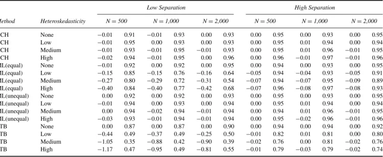
We now discuss the bias-adjusted three-step approaches for dealing with continuous distal outcomes. These proceed as follows:

1. Build a standard LC model based on the categorical response variables (Figure 3a).

2. Assign individuals to latent classes (Figure 3b). The assigned class memberships are denoted byW. 3. Estimate the association betweenX andZ using the

assigned class memberships W, taking into account that these contain classification errors (Figure 3c).

In the first step, a model is built for response variables

Yi using the basic LC model described in Equation 3 and

depicted in Figure 3a. In the second step, individuals are assigned to latent classes based on their posterior class

(a) (b) (c)

FIGURE 3 The three steps of the bias-adjusted three-step approaches.

membership probabilitiesW. These are calculated from the parameters of the Step 1 model using Bayes rule; that is,

P(X=t|Yi)=

P(X=t)P(Yi|X=t)

P(Yi)

. (10)

Two possible assignment rules are modal and proportional assignment, which in cluster analysis terminology yield a hard and a soft partitioning, respectively (Dias & Vermunt,

2008). In modal assignment, each individual is assigned to a single class; that is, the class for which the posterior member-ship probability is largest. This can be expressed as follows: P(W =s|Yi) = ifP(X=s|Yi)>P(X=t|Yi) for alls=t

and equals to 0 for the other classes. In proportional assign-ment, each individual is assigned to each of the classes with a weight equal toP(W =s|Yi)=P(X=s|Yi). In practice, this

implies that subsequent analyses should be performed using an expanded data withT records for each unit, with records weights equal toP(W=s|Yi).

Irrespective of the assignment method used, classifica-tion errors will be present unless the classificaclassifica-tion is perfect (Bolck et al.,2004). By aggregating over the observed data patterns, the amount of errors can be expressed as the prob-ability of an assigned class membershipsconditional on the true class membershipt(Bakk et al.,2013; Vermunt,2010),

P(W =s|X=t)=

N

i=1

P(X=t|Yi)P(W =s|Yi)

N P(X=t) . (11)

Lastly, in the third step, the class assignments W are used to estimate the relation betweenXandZwhile correct-ing for the known classification errors introduced in Step 2 (Figure 3c). This is achieved using a model of the form (Bakk et al.,2013):

P(W =s,Zi)= T

t₌1

P(X=t)f(Zi|X=t)P(W=s|X=t).

(12)

Note that this is an LC model in which Z and W are used as response variables, and in whichP(W =s|X=t) is fixed. The model described in Equation 12 can be either esti-mated using maximum likelihood estimation (yielding the ML approach) or using a weighted analysis as proposed by Bolck, et al. (yielding the BCH approach; Bolck et al.,2004; Vermunt,2010). These two approaches are presented in more detail in the following.

The ML Approach

The ML approach estimates the LC model defined in Equation 12 directly. TheP(W =s|X=t) are fixed to their estimated values from the second step (see Equation 11),

(6)

whereas the parameters in the part of interest,f(Zi|X =t),

are freely estimated. To be able to estimate the class-specific means μt, we need to specify the distributional form of

f(Zi|X =t), which for continuousZis usually defined to be

a normal distribution. The variance ofZ can be modeled as either equal or unequal across classes, which we refer to as the ML(equal) and ML(unequal) approaches. SE estimates for the free parameters are obtained based on the robust estimator, which is especially needed when proportional assignment is used (Bakk, Oberski, & Vermunt,2014). Tests for the equality of means can be performed using Wald tests. The ML approach yields unbiased estimates of the μt

and their standard errors when normality assumption holds (Bakk et al.,2014, Bakk et al.,2013). However, the approach could fail when this assumption is violated. For example, when Z has a bimodal distribution within the classes, the Step 3 LC model might pick up this bimodality inZ, which will fully distort the original definition of the latent classes (Asparouhov & Muthén,2014). To decrease the likelihood of obtaining a completely different LC solution, both in the Mplus7.1 and the Latent GOLD 5.0 implementation-specific starting values are used for the Step 3 model1. In this way, a local maximum of the likelihood is obtained with class defi-nitions that are closer to those of first-step model than of the global maximum (Asparouhov & Muthén,2014)2.

The ML approach could also lead to biased estimates for μtif the error variance is wrongly assumed to be equal across

the classes. However, it is less clear how problematic such a misspecification will be. In the simulation study, we inves-tigate the impact of bimodality and of wrongly assuming homoskedastic variances when they are heteroskedastic.

The BCH Approach

Whereas ML approach estimates the LC model defined in Equation 12 directly, the BCH approach transforms the prob-lem and estimates an ANOVA model with observed variables only. It re-creates the true latent classification by weighting W with the inverse of the classification errors (Bolck et al.,

2004; Vermunt, 2010). The resulting model is estimated using a pseudo maximum likelihood estimation procedure. To account for the multiple (T) records per individual and for the weighting, robust standard errors should be used (Bakk et al, 2014; Vermunt,2010). The equality of class-specific means is tested using Wald tests.

1_{Note that the ML approach is called 3step in M}_plus_{7.1 and is an option}

of ‘Auxiliary’

2_M_plus_{7.1 estimates the Step 3 model using as starting values the}

esti-mated class sizes from the first step, whereas Latent GOLD 5.0 fixes these values. For the means of Z, Mplus7.1 uses the unadjusted class-specific means, whereas Latent GOLD 5.0 starts using the overall mean and vari-ance ofZfor all classes. Due to this different implementation, in some cases different results can be obtained, although this is rare and occurs mainly in situations where the use of the ML approach is anyway not recommended.

An important advantage of the BCH approach compared to the ML approach is that the class definitions will not change when the distribution of Z is misspecified. The reason for this is that it involves performing an ANOVA-like analysis with observed variables only rather than estimating an LC model. Moreover, a positive side effect of using robust SEs is that these correct for all kinds of misspecifications, thus also for a possible misspecification of the distribution of the errors. This means, for example, that Wald tests for the class-specific means are identical irrespective of whether one assumes homoskedastic or heteroskedastic errors. So, we can simply assume equal error variances when using the BCH approach.

A possible problem associated with the BCH approach, which could occur with very low class separation and small sample sizes, is that the error variance might become nega-tive in one or more classes when these variances are specified to be unequal across classes. In these situations, it is rec-ommended not to use the BCH approach with class-specific variances. A similar problem was reported by Bakk et al. (2013) for nominal outcomes, where negative cell frequen-cies could be found. However, negative variances will not occur when using the BCH method with equal variances, which is therefore the preferred approach.

The BCH approach is available in Latent GOLD 5.0, with the default specification for continuous distal outcomes being the one with equal variances. The Mplus7.1 version available at the time we performed this research did not implement the BCH approach, but we were notified that it will become available in the next version.

A Comparison of the Underlying Assumptions of the Stepwise Approaches and the Possible

Consequences of Violating These Assumptions

Table 1 summarizes the assumptions of the various approaches and the possible consequences of their viola-tions. As can be seen, for certain assumptions it is known that their violation will have an impact on the estimated class-specific means, their SEs, or both. For example, viola-tion of the normality assumpviola-tion, such as when class-specific distributions are bimodal, might bias the results obtained with the ML method (Asparouhov & Muthén,2014). It is also known that plugging in the parameter values from Step 1 without accounting for their sampling fluctuation can lead to underestimated SEs when using the three-step approaches (Bakk et al.,2014). The same seems to apply to the some-what ad hoc SE estimates proposed by Asparouhov and Muthén (2014) for the LTB approach. However, the extent of these effects has not systematically been investigated so far. Moreover, for some of the assumptions it is unknown whether their violation will cause bias. For instance, we do not know how strongly the LTB method is affected by a possible logistic nonlinearity of the trueZ–Xassociation.

(7)

TABLE 1

Underlying Assumptions of the Stepwise Latent Class Analysis Approaches and Hypothesized Consequences of Their Violation

BCH ML(equal) ML(unequal) LTB

Assumptions

Normal distribution Yes Yes Yes No Linear-logisticZ-X

relationship

No No No Yes

Equal variances Yes Yes No Yes No uncertainty in Step 1

parameters

Yes Yes Yes Yes

Violation hypothesized to affect

Normal distribution None Means, SEs Means, SEs — Linear-logisticZ-X

relationship

— — — Means

Equal variances None Means, SEs — Means No uncertainty in Step 1

parameters

SEs SEs SEs SEs

Note.SE=Standard error.

SIMULATION STUDY

The goal of the simulation study is to compare the differ-ent stepwise LC methods for dealing with continuous distal outcomes with regard to their robustness against violations of underlying assumptions. We focus on the assumptions summarized inTable 1. More specifically, we generated data under different degrees of bimodality and heteroskedasticity. Bimodality violates the assumption of normality made by the BCH and the two ML approaches. Heteroskedasticity vio-lates the assumption of equal variances of the ML (equal) approach and the assumption of logistic linearity of the LTB method. We not only investigate bias, but also the quality of the SE estimates provided by the various stepwise methods. The results of two studies are presented: In the first study we focus solely on bias, whereas in the second study the consequences of sampling fluctuation are also considered.

Study 1

In Study 1, we investigated the bias in the estimated class-specific means of the distal outcome for each of the stepwise methods. The population model was two-class model for six dichotomous response variables. Class sizes were set to be equal. The class-specific probability of a positive answer was set to .80 in Class 1 for all indicators, and to .20 in Class 2, corresponding to an entropy-basedR2 _{value of .82.}

Both modal and proportional assignment were used when applying the three-step approaches.

Furthermore, we manipulated the degree of heteroskedasticity and bimodality in the class-specific distribution ofZ. We defined four conditions with gradually increasing degrees of heteroskedasticity. We set the variance in Class 1 equal to 1, and in Class 2 equal to 1, 4, 9, and 25, respectively, thus going from equal to highly unequal

variances. In addition, we defined three conditions with gradually increasing degrees of bimodality. In Class 1,Zwas assumed to come from the mixture of normal distributions of the form 0.75N(−2,τ2₎₊_0.25N(2,_τ2_{), thus having}

a class-specific mean of −1. In Class 2, Z followed the mixture distribution 0.75N(2,τ2)+0.25N(−2,τ2), thus having a class-specific mean of 1. The degree of bimodality was manipulated by setting the variance σ2 to either 0.01, 0.50, or 1, which affects the overlap between the mixing distributions. In this way, conditions were created without any overlap at all and thus extreme bimodality (τ2₌_0.01),

some overlap and thus moderate bimodality (τ2₌_0.50),

and large overlap and thus nonextreme bimodality (τ2₌_1).

In all investigated conditions, we generated a single data set with 1,000,000 observations. For each condition and each estimator, we determined the bias in the difference in means between the two classes (the true difference is 2). The ML estimator was applied with equal and unequal variances, and for both of these methods we used versions with random and with predefined starting values. Because results were very similar for modal and proportional assignment, we report only the results obtained with modal assignment.

Table 2 summarizes the results for the four heteroskedasticity conditions. As can be seen in the first row, when the variances are equal between the two classes, all the methods perform well. This result is similar to what was found in previous simulation studies (Asparouhov & Muthén, 2014, Bakk et al., 2013; Lanza et al., 2013). However, as the degrees of heteroskedasticity increase (vari-ance in Class 2 increases), the ML(equal) estimate becomes more strongly biased. The ML approach with random starting values shows larger bias than its counterpart with predefined starting values. At the same time, the BCH and the ML(unequal) approaches obtain unbiased estimates in all conditions. The estimates obtained with the LTB approach have a small bias when the variances are unequal, which shows that the method is indeed affected by the relationship betweenZandXbeing nonlinear on the logit scale.

Table 3summarizes the conditions whereZhas a bimodal within-class distribution. In all three conditions, the BCH and LTB methods obtain the correct class-specific means. In contrast, the ML approaches are highly sensitive to bimodality. When the bimodality becomes more extreme, the bias of the ML estimates increases. The ML approaches with prespecified starting values show somewhat smaller bias than their counterparts with the random starting values.

In summary, the LTB and the ML (equal) approaches yielded biased estimates when variances are unequal between classes. Moreover, both ML approaches were sen-sitive for bimodality. The ML approaches with prede-fined starting values (as implemented as default setting in Mplus 7.1 and LatentGOLD 5.0) performed some-what better than their counterparts with random start-ing values. The BCH approach performed well in all conditions.

(8)

TABLE 2

Absolute Bias in the Estimated Difference of Means Obtained With the Stepwise Latent Class Methods for Varying Degrees of Heteroskedasticity Using Modal Assignment in Study 1

Heteroskedasticity BCH

ML (equal, nonrandom)

ML(unequal, nonrandom)

ML(equal, random)

ML(unequal,

random) LTB

None 0.00 0.00 0.00 0.00 0.00 0.00

Low 0.00 0.15 0.00 0.19 0.00 0.04

Medium 0.01 0.05 0.01 0.06 0.01 0.04

High 0.00 0.10 0.00 0.11 0.00 0.03

TABLE 3

Absolute Bias in the Estimated Difference of Means Obtained With the Stepwise Latent Class Methods for Varying Degrees of Bimodality Using Modal Assignment in Study 1

Bimodality BCH

ML(equal, nonrandom)

ML(unequal, nonrandom)

ML(equal, random)

ML(unequal,

random) LTB

Low 0.00 0.11 0.11 0.11 0.11 0.01

Medium 0.00 0.12 0.12 0.12 0.12 0.01

High 0.01 0.21 0.21 2.00 2.00 0.01

Study 2

In the following, we compare the different methods using a larger and more realistic LC model and, moreover, account-ing for samplaccount-ing fluctuation. Given that the ML methods with random starting values proved to be more biased than their counterparts that use predefined starting values, we restrict ourselves to the latter implementation.

Data were generated from a four-class model with eight dichotomous indicators, with parameter values based on the application to psychological contract types described by Bakk et al. (2013). The class sizes were set to .50, .30, .10, and .10, similarly to this real data example used as starting point. In Class 1, all indicators have a high probability of a positive answer, whereas in Class 2 the first four indica-tors have a high probability of a positive answer, and the last four of a negative answer. At the same time, in Class 3 the first four indicators have a low probability of a posi-tive answer, whereas the last four have a high probability of a positive answer, and in Class 4 all indicators have a low probability of a positive answer. We manipulated the class separation by setting the probability of a positive answer to .80 (.20) or .90 (.10), which yields a moderate and a high separation condition.

The class-specific means of the distal outcome were set to −1, −0.5, 0.5, and 1, respectively. Similarly to Study 1, we looked into two types of situations: unequal class-specific variances of Z (heteroskedasticity) and bimodal class-specific distributions ofZ. More specifically, the con-ditions with heteroskedasticity were created by setting the variance ofZto 1, 4, 9, and 25 in Classes 2 and 3, while keep-ing it equal to 1 in Classes 1 and 4. The bimodal conditions were defined such that Classes 2 and 3 have bimodal distribu-tions, whereas Classes 1 and 4 have unimodal distributions.

The bimodality was again obtained by using the mixture distribution: 0.75N(−1,τ2₎₊_0.25N(1,_τ2_{) in Class 2 and}

0.75N(1,τ2₎₊_0.25N(₋_1,_τ2_{) in Class 3. We manipulated}

the extremeness of the bimodal distributions by settingτ2

equal to 1, 0.5, and 0.01.

Three sample size conditions were investigated: 500, 1,000, and 2,000. For all conditions, 500 replications were used. The bias in class-specific means and the coverage rate based on the SE estimates were investigated for the LTB, BCH, ML(equal), and ML(unequal) approaches. We con-sider an estimator to perform well if it has a bias close to 0 and a coverage rate close to .95.

Results Under Heteroskedasticity

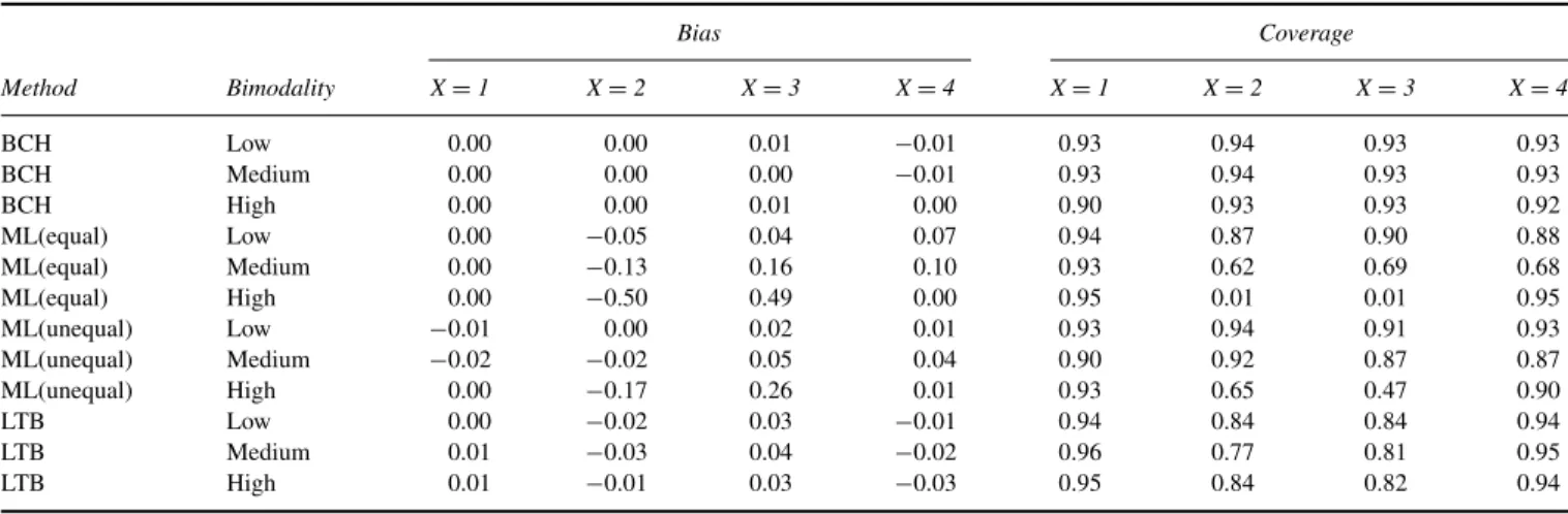
Table 4 shows the results averaged across separation level and sample size conditions for all levels of heteroskedasticity. Note that the four different levels of heteroskedasticity (none, small, medium, and large) cor-respond with a variance of 1, 4, 9, and 25 in Classes 2 and 3. Similar to Study 1, the estimates obtained with the BCH approach are unbiased in all conditions. Moreover, coverage rates are between .93 and .95, thus slightly too low in some conditions. Also the ML approaches yield results comparable to Study 1. That is, in all conditions the estimates obtained with the ML(unequal) approach are unbiased. Coverage rates are between .93 and .95. With ML(equal), the estimates are highly biased.

At the same time, the LTB estimates are increasingly biased as the degree of heteroskedasticity increases. Whereas the first class is hardly affected by this bias, the other classes are strongly affected, especially Class 2. The cover-age rates obtained with LTB are too low even in the none heteroskedastic condition (between .86 and .91), although

(9)

TABLE 4

Bias and Coverage Rate for Class-Specific Means Averaged Across Separation Level and Sample Size Conditions For Different Degrees of Heteroskedasticity: Study 2

Bias Coverage

Method Heteroskedasticitv X=1 X=2 X=3 X=4 X=1 X=2 X=3 X=4

BCH None 0.00 0.00 0.01 −0.01 0.94 0.94 0.94 0.93

BCH Low 0.00 0.00 0.01 0.01 0.94 0.94 0.94 0.94

BCH Medium 0.00 0.00 0.00 0.00 0.94 0.94 0.95 0.94

BCH High 0.00 −0.01 0.01 0.00 0.94 0.96 0.94 0.94

ML(equal) None 0.00 0.00 0.00 −0.01 0.94 0.93 0.93 0.93

ML(equal) Low 0.01 −0.01 0.01 0.17 0.94 0.84 0.91 0.77

ML(equal) Medium 0.02 −10.18 −0.05 0.36 0.93 0.81 0.90 0.70

ML(equal) High 0.03 −0.24 −0.12 0.53 0.93 0.86 0.89 0.77

ML(unequal) None 0.00 0.00 0.00 −0.01 0.94 0.93 0.92 0.93

ML(unequal) Low 0.00 0.00 0.00 −0.01 0.94 0.94 0.93 0.94

ML(unequal) Medium 0.00 0.00 0.00 0.00 0.95 0.94 0.94 0.94

ML(unequal) High 0.00 −0.01 −0.01 0.00 0.94 0.95 0.94 0.95

LTB None 0.00 0.00 0.00 0.00 0.91 0.88 0.86 0.86

LTB Low 0.00 −0.18 0.11 0.00 0.97 0.65 0.71 0.94

LTB Medium −0.02 −0.48 0.22 0.12 0.94 0.58 0.64 0.83

LTB High −0.03 −0.50 0.21 0.29 0.91 0.64 0.64 0.86

TABLE 5

Bias and Coverage Rate for the Mean of Class 2 Per Separation Level and Sample Size Condition for Different Degrees of Heteroskedasticity: Study 2

Low Separation High Separation

Method Heteroskedasticity N=500 N=1,000 N=2,000 N=500 N=1,000 N=2,000

BCH None −0.01 0.91 −0.01 0.93 0.00 0.93 0.00 0.95 0.00 0.93 0.00 0.95 BCH Low −0.01 0.95 0.00 0.93 0.00 0.93 0.00 0.95 0.01 0.94 0.00 0.94 BCH Medium −0.01 0.93 −0.01 0.95 −0.01 0.93 0.00 0.95 0.01 0.96 −0.01 0.95 BCH High −0.02 0.94 −0.01 0.95 0.00 0.96 0.00 0.96 −0.01 0.97 −0.01 0.96 ML(equal) None −0.01 0.92 0.00 0.92 0.00 0.95 0.00 0.94 0.00 0.93 0.00 0.95 ML(equal) Low −0.15 0.85 −0.15 0.76 −0.16 0.64 −0.05 0.94 −0.04 0.93 −0.05 0.91 ML(equal) Medium −0.27 0.80 −0.29 0.72 −0.31 0.54 −0.07 0.94 −0.07 0.95 −0.09 0.89 ML(equal) High −0.40 0.84 −0.40 0.77 −0.42 0.68 −0.07 0.96 −0.08 0.97 −0.08 0.93 ML(unequal) None 0.00 0.92 0.00 0.92 0.00 0.93 0.00 0.95 0.00 0.93 0.00 0.95 ML(unequal) Low −0.01 0.94 0.00 0.93 0.00 0.94 0.00 0.95 0.01 0.94 0.00 0.94 ML(unequal) Medium 0.00 0.94 −0.02 0.94 −0.01 0.94 0.00 0.94 0.01 0.96 −0.01 0.95 ML(unequal) High −0.03 0.93 −0.01 0.94 −0.01 0.94 0.00 0.95 −0.02 0.96 −0.01 0.96 LTB None 0.00 0.87 0.00 0.87 0.00 0.90 0.00 0.94 0.00 0.94 0.00 0.92 LTB Low −0.44 0.49 −0.37 0.49 −0.25 0.50 −0.01 0.82 0.01 0.81 0.00 0.80 LTB Medium −1.05 0.35 −0.88 0.42 −0.90 0.39 −0.02 0.76 0.00 0.81 −0.02 0.76 LTB High −1.17 0.47 −0.95 0.49 −0.81 0.55 −0.01 0.79 −0.03 0.79 −0.02 0.74

the estimated class-specific means are unbiased. This shows that the undercoverage is the result of an underestimation of the SEs.

Table 5presents the bias and coverage rate for the mean of Class 2, but now separately for each separation level and sample size condition. We chose to give the detailed results only for the mean of Class 2 because this parameter showed the largest bias. For all methods at hand, it can be seen that as uncertainty increases (smaller sample size and lower sep-aration), the bias increases and the coverage rate decreases. Only the BCH approach obtains almost unbiased estimates and good coverage rates in all conditions. However, even this

method obtains a somewhat too low coverage rate with low separation and small sample size (between .91 and .93), thus showing that the SEs are somewhat underestimated in these situations.

It can be seen that the LTB method is very sensitive to the stability of the Step 1 model: In the low separation conditions the bias is extremely large, Whereas in the high separation conditions the bias is negligible. The coverage rates with the LTB approach are clearly too low (between .87 and .94), even in the conditions with equal variances, which shows that the SEs are underestimated. At the same time, the ML methods are less affected by the class separation. If the variance ofZis

(10)

correctly specified, the ML estimates are unbiased in all con-ditions, obtaining a coverage rate between .92 and .94 (thus having a minor undercoverage). However, if the variances are wrongly assumed to be equal, the bias is always large.

Results With Bimodality

Let us now look at the results for the three bimodality condi-tions, which are presented inTable 6. These are again aver-ages across sample size and separation level conditions. The BCH estimates are unbiased in all conditions and their cov-erage rates are between .90 and .94, with the lowest covcov-erage rates occurring in the most extreme bimodality condition.

At the same time, the ML(equal) approach fails when the bimodality is the most extreme, but as the bimodality becomes less extreme the bias decreases. The bias in the ML(unequal) estimates is lower than in those of ML(equal). However, even the ML(unequal) estimates are much worse than the LTB and BCH estimates. Both ML approaches

show much too low coverage rates, but these are in fact uninformative given that these estimates are biased any-how. Furthermore, the LTB approach yields estimates with very small bias; however, the coverage rate is again too low (.77 at its worst), especially in Classes 2 and 3, which have a bimodally distributedZ.

Table 7presents the results for the mean in Class 2, but now separately per sample size and separation condition. The BCH approach is unbiased. In the low separation conditions, it has a coverage rate between .89 and .93. However, in the high separation condition, the coverage rate is better.

The ML methods fail with the most extreme bimodality, which is also what we saw in Study 1. As the bimodality becomes less extreme, the estimates obtained using ML(unequal) become less biased. This tendency depends solely on the amount of bimodality and not on separation level or sample size. At the same time, using the LTB method, the bias is small in all conditions. However, in the low separation conditions, the coverage rate is too low, irrespective of the sample size.

TABLE 6

Bias and Coverage Rate for the Class-Specific Means Averaged Across Separation Level and Sample Size Conditions for Different Degrees of Bimodality: Study 2

Bias Coverage

Method Bimodality X=1 X=2 X=3 X=4 X=1 X=2 X=3 X=4

BCH Low 0.00 0.00 0.01 −0.01 0.93 0.94 0.93 0.93

BCH Medium 0.00 0.00 0.00 −0.01 0.93 0.94 0.93 0.93

BCH High 0.00 0.00 0.01 0.00 0.90 0.93 0.93 0.92

ML(equal) Low 0.00 −0.05 0.04 0.07 0.94 0.87 0.90 0.88

ML(equal) Medium 0.00 −0.13 0.16 0.10 0.93 0.62 0.69 0.68

ML(equal) High 0.00 −0.50 0.49 0.00 0.95 0.01 0.01 0.95

ML(unequal) Low −0.01 0.00 0.02 0.01 0.93 0.94 0.91 0.93

ML(unequal) Medium −0.02 −0.02 0.05 0.04 0.90 0.92 0.87 0.87

ML(unequal) High 0.00 −0.17 0.26 0.01 0.93 0.65 0.47 0.90

LTB Low 0.00 −0.02 0.03 −0.01 0.94 0.84 0.84 0.94

LTB Medium 0.01 −0.03 0.04 −0.02 0.96 0.77 0.81 0.95

LTB High 0.01 −0.01 0.03 −0.03 0.95 0.84 0.82 0.94

TABLE 7

Bias and Coverage Rate for the Mean of Class 2 Per Separation Level and Sample Size Condition for Different Degrees of Bimodality: Study 2

Low Separation High Separation

Method Bimodality N=500 N=1,000 N=2,000 N=500 N=1,000 N=2,000

BCH Low 0.00 0.94 −0.01· 0.94 −0.01 0.91 0.01 0.95 −0.01 0.94 −0.01 0.97 BCH Medium 0.00 0.94 0.00 0.93 0.00 0.91 0.00 0.95 0.00 0.96 0.00 0.95 BCH High 0.00 0.89 0.00 0.91 0.00 0.91 0.00 0.96 0.00 0.95 0.00 0.94 ML(equal) Low −0.07 0.89 −0.08 0.83 −0.09 0.71 −0.02 0.95 −0.03 0.91 −0.03 0.92 ML(equal) Medium −0.18 0.62 −0.20 0.42 −0.20 0.22 −0.07 0.89 −0.07 0.82 −0.07 0.73 ML(equal) High −0.50 0.00 −0.50 0.00 −0.50 0.00 −0.48 0.03 −0.49 0.01 −0.50 0.00 ML(unequal) Low 0.00 0.93 −0.01 0.92 −0.01 0.90 0.01 0.96 −0.01 0.94 −0.01 0.96 ML(unequal) Medium −0.03 0.91 −0.02 0.90 −0.02 0.87 −0.01 0.96 −0.01 0.96 0.00 0.95 ML(unequal) High −0.25 0.42 −0.30 0.38 −0.33 0.35 −0.05 0.92 −0.05 0.92 −0.04 0.91 LTB Low −0.04 0.78 −0.03 0.78 −0.03 0.76 0.00 0.92 −0.01 0.92 −0.01 0.91 LTB Medium −0.08 0.67 −0.06 0.65 −0.05 0.63 −0.01 0.89 −0.01 0.90 0.00 0.89 LTB High −0.04 0.76 −0.02 0.79 −0.02 0.76 0.00 0.92 −0.01 0.91 0.00 0.88

(11)

All in all, we see that the ML approaches fail when Z has a bimodal distribution within classes. At the same time, in the heteroskedastic variance conditions, estimated class-specific means obtained with the ML approach are unbiased if the variance is modeled correctly. This shows that the ML methods are very sensitive to misspecification when dealing with continuous distal outcomes. The LTB approach turns out to yield biased estimates when the underlying assump-tion of logistic linearity is violated. In all condiassump-tions, the method that obtained the least biased estimates was the BCH approach. All investigated approaches yield too low cover-age rates in the higher uncertainty conditions; that is, when class separation is lower and sample size is smaller.

EMPIRICAL EXAMPLE: RECIDIVISM OF LATENT CLASSES OF JUVENILE OFFENDERS

To illustrate the stepwise LC modeling approaches we use a data set on juvenile offenders’ recidivism from the Dutch Ministry of Justice, which was analyzed earlier by Mulder et al. (2012) using unadjusted three-step LC anal-ysis. Although these authors were aware of the fact that this approach could yield biased estimates, for them it was the only way to proceed given the large number (70) of dis-tal outcomes, which cannot be dealt with using a one-step approach (Mulder et al.,2012), and given that bias-adjusted approaches were not available at that time.

As did Mulder et al. (2012), we built an LC model using 13 categorical indicators, representing the offense frequency prior to conviction (grouped into three categories: low. aver-age, and high) and 12 types of offenses (yes–no). The model selected based on the Baycsian Information Criterion (BIC) is the four-class model (BIC =–3769), which turns out to be a rather strong clustering model in terms of class separa-tion (entropy-basedR2=.75). The four groups are, as shown inTable 8, the violent property offenders (being differenti-ated from the other groups by high scores on the property offenses and misdemeanor, and a high number of offenses), the property offenders (similar to the first group, but lower offense rates), the serious violent offenders (with high scores on manslaughter and murder), and the sexual offenders (with high scores on sexual offenses with same age victims and pedophilic offenses).

Whereas Mulder et al. (2012) built the Step 1 model using the full sample of 1,082 respondents, we used a subsample of 728 respondents. This is the subsample for which recidivism information is available; that is, meeting the requirement of having been released to the community for a minimum of 2 years at the time of the data collection. We used this sub-sample instead of the full sub-sample because the LTB approach requires that the distal outcomes are observed for all units. For comparability of results, the same sample was used for the three-step approaches as well, although for these

TABLE 8

Profile of Latent Classes of Juvenile Offenders

Violent Property Property Serious Violent Sexual

Class proportion 0.46 0.29 0.15 0.10 Number of offenses

Low 0.00 0.32 0.73 0.80

Medium 0.30 0.45 0.27 0.18

High 0.70 0.24 0.00 0.02

Misdemeanor 0.56 0.08 0.20 0.05

Drugs 0.06 0.03 0.05 0.00

Vandalism 0.00 0.00 0.00 0.00

Property 0.99 1.00 0.28 0.17

Moderate violent 0.91 0.36 0.74 0.15 Violent property 0.63 0.82 0.18 0.01 Serious violent 0.41 0.05 0.24 0.00 Sexual same age 0.14 0.04 0.11 0.63

Pedosexual 0.04 0.00 0.00 0.61

Manslaughter 0.08 0.03 0.43 0.06

Arson 0.05 0.00 0.10 0.00

Murder 0.01 0.01 0.18 0.03

approaches it is no problem to base the third step analysis on a subsample of the sample used to build the LC model.3

We computed the class-specific means and their SEs of two distal outcome variables, the frequency and severity of recidivism, using the stepwise LC methods (seeTable 9). The overall Wald test indicates that there is a significant differ-ence between the class-specific means of the frequency of recidivism with all methods at hand. It can be seen that as a result of the attenuation effect, the differences between the classes are somewhat smaller for the unadjusted three-step approach. Irrespective of the method used, violent property offenders have the highest recidivism frequency, followed by the property offenders. All methods except ML (unequal) obtain a somewhat higher class-specific mean for the serious violent offenders than for sexual offenders, whereas this lat-ter method reverses the order of these two groups. This might be the result of the fact that ML(unequal) is more strongly affected by arbitrary deviations from within-class normal-ity. The estimated class-specific means are similar for BCH and ML (equal), but somewhat different from LTB estimates. This might indicate that the linear-logistic assumption is vio-lated to a certain extent. Note also that the SEs obtained with the LTB approach are smaller than those of the bias-adjusted three-step methods and sometimes even smaller than those of the unadjusted three-step analysis. This confirms that the LTB SEs are probably underestimating the actual sam-pling variability in the reported class-specific means. Also for severity of recidivism, the overall Wald test shows a sig-nificant difference in means across classes for all methods at hand. Moreover, again the differences between the classes are somewhat smaller for the unadjusted three-step approach.

3_{The model parameters obtained with 1,082 observation are very}

simi-lar, which is probably the result of the measurement model being strong.

(12)

TABLE 9

Mean and Standard Error of Frequency and Severity of Recidivism for the Four Offender Classes Obtained With Five Stepwise Latent

Class Approaches

Violent Property Property Serious Violent Sexual

Frequency of recidivism

Unadjusted 9.85 (.62) 6.08 (.53) 3.33 (.58) 2.78 (.54) BCH 10.46 (.72) 5.73 (.65) 3.03 (.65) 2.74 (.57) ML (equal) 10.39 (.65) 5.69 (.48) 3.31 (.49) 2.83 (.5l) ML (unequal) 12.72 (.76) 3.50 (.51) 1.31 (.47) 3.07 (.61) LTB 10.15 (.66) 5.92 (.50) 3.27 (.40) 2.81 (.43) Severity of recidivism

Unadjusted 5.60 (.17) 4.80 (.22) 3.75 (.33) 2.13 (.34) BCH 5.73 (.20) 4.77 (.26) 3.75 (.38) 2.02 (.36) ML (equal) 5.74 (.20) 4.76 (.27) 3.72 (.39) 2.03 (.35) ML (unequal) 5.73 (.20) 4.76 (.27) 3.83 (.40) 1.89 (.50) LTB 5.69 (.17) 4.79 (.22) 3.76 (.30) 1.98 (.31)

The severity is highest among violent property offenders, followed by property offenders, violent offenders, and sex-ual offenders. Note that all adjusted methods give almost the same class-specific means, showing that assumption viola-tions are not a problem here. SE estimates are again probably too low for the LTB approach.

CONCLUSIONS AND DISCUSSION

We investigated the robustness of four stepwise LC anal-ysis methods for studying the relationship between class membership and continuous distal outcomes. The BCH method, the ML method with equal variances, and the ML method with unequal variances are bias-adjusted three-step approaches, which assume that the distal outcome is normally distributed, whereas ML(equal) also assumes homoskedasticity. The LTB method, which obtains the class-specific means of the distal outcome by estimating an LC model in which the distal outcome is treated as a covariate, assumes that the relationship between the distal outcome and class membership is linear on a logistic scale.

In a simulation study, we investigated the perfor-mance of the stepwise methods under different degrees of heteroskedasticity and bimodality of the class-specific dis-tributions of the distal outcome. Bimodality is a violation of the assumption of normality needed for the BCH and ML approaches; heteroskedasticity violates the assumption of logistic linearity of the LTB approach, and the assump-tion of homoskedasticity of the ML approach with equal variances. The simulation results revealed that the BCH method is the most robust approach: It yielded unbiased estimates under all investigated conditions. This is most probably the result of the fact that it involves performing a weighted ANOVA, a method that is known to be robust against violations of assumptions. The other methods are sensitive to the violations considered. The ML approach fails to different degrees in all the situations investigated.

When the variance is heteroskedastic, modeling it as equal between the classes produces a bias in the class-specific means. However, if the heteroskedasticity is correctly mod-eled, the ML method works fine. The ML approach cannot handle bimodal class-specific distributions of the outcome variable and probably any other departure from normality as well.4 The LTB approach yields biased estimates of the class-specific means when the errors are heteroskedastic, and shows a small bias with certain conditions of bimodality.

All four methods yielded coverage rates lower than the nominal .95 rate when the separation between classes is low and the sample size is small. For the three-step approaches, the too low coverage rate is caused by ignoring the uncer-tainty about the fixed parameter estimates from Step 1 (Bakk et al.,2014). However, by taking this uncertainty into account, coverage rates close to the nominal .95 level can be obtained, as shown by Bakk et al. (2014) for the ML approach. For the LTB approach, a somewhat ad hoc SE esti-mator was used, which turned out to yield a too low coverage in all investigated conditions; the undercoverage increases when the uncertainty about the Step 1 parameters and about the class memberships increases.

Because it performed very well in all investigated conditions, we recommend using the BCH approach for stepwise LC modeling with continuous distal outcomes. The use of the ML methods with continuous distal outcomes is recommended only with precaution due to its sensitivity to assumption violations. We also recommend caution with the LTB method, both due to the bias that can occur with heteroskedastic errors and due to the undercoverage resulting from the current SE estimates. The application to the juvenile recidivism data showed that results might indeed differ depending on the method that is used. It seems to be safest to rely on the results obtained with the very robust BCH approach.

Although in this article we focused on the performance of stepwise LC analysis approaches for the simple case in which one studies the relationship between class mem-bership and a single continuous distal outcome, it should be mentioned that these approaches can also be used in much more general situations. The ML and BCH three-step approaches are very flexible, and can, for instance, also be applied with covariates (Vermunt, 2010), with multiple latent variables (Bakk et al,2013), with continuous indica-tors (Gudicha & Vermunt,2011), with latent Markov models (Vermunt & Magidson,2013), and with multilevel models (Bennink, Croon, & Vermunt,2014), as well as with models combining these features; for example, a regression model for a continuous distal outcome in which not only the LC variable but also other predictors are included, or a structural equation model in which the LC variable is predicted by

4_{Note that M}_plus_{gives a warning when the definition of the classes}

changes due to deviations from normality. When this problem occurs, the BCH approach should clearly be preferred.

(13)

other variables and is itself a predictor of one or more dis-tal outcomes. Although all these possibilities exist and are available in software, there is a need for further research into the performance of the stepwise approaches in these more complex setups. For example, in models in which variance estimates are of interest, one should investigate the effect of the negative weighting used in BCH on the parameter esti-mates. It should be stressed that the LTB approach is more limited in the sense that it can only be used for the situa-tion in which there is a single distal outcome, the situasitua-tion investigated in this article. It should, however, be mentioned that it can also be used with distal outcomes that are not continuous (Lanza et al,2013). When used with categorical outcomes, the problems reported here do not occur and the LTB approach can be used without any concern.

Future research might focus on improving the recently proposed LTB method in various ways. First, it seems to be possible to prevent the encountered bias by expanding the logistic part of the model with quadratic and higher order terms. Moreover, the undercoverage problem could be resolved by using better SE estimates; for instance, SEs obtained by bootstrapping. It might also be useful to trans-form the LTB approach into a true stepwise approach, in which as in the three-step approaches the estimation of the LC model and the investigation of the association between classes and distal outcomes are fully separated. This would prevent the need to reestimate the original LC model for each distal outcome. Moreover, it would also make it possible to base the distal outcome analysis on a subsample, as was actually needed in our real data example, or even on a fully different sample, as would be the case when the classification information is obtained from an earlier study.

Another area that needs further attention are the some-what underestimated BCH SEs in the conditions with small sample size and low class separation. The SE estimates could be corrected for by accounting for the uncertainty in the BCH weights, which are computed using the Step 1 parameter estimates, similar to the correction proposed for the ML approach by Bakk et al. (2014). Another possible solution could be to switch to bootstrap SEs in these conditions. It should then be investigated whether bootstrapping in Step 3 only suffices, or whether it is needed in Step 1 as well.

A limitation of our study is that we focused on problems associated with heteroskedasticity and bimodality. It is rec-ommended for future research to analyze whether other types of violations of normality, such as skewness, excess kurtosis, and outliers, are problematic for the stepwise approaches at hand. We hypothesize that such violations will have only a minor effect on the rather robust BCH approach, whereas they could bias parameter estimates of the ML and LTB methods to varying degrees.

REFERENCES

Agresti, A. (2002).Categorical data analysis(2nd ed.). New York, NY: Wiley.

Asparouhov, T., & Muthén, B. (2014). Auxiliary variables in mixture modeling: Three-step approaches using Mplus. Structural Equation Modeling,21, 329–341.

Bakk, Z., Oberski, D., & Vermunt, J. (2014). Relating latent class assign-ments to external variables: Standard errors for correct inference.Political Analysis,22, 520–540.

Bakk, Z., Tekle, F. T., & Vermunt, J. K. (2013). Estimating the association between latent class membership and external variables using bias-adjusted three-step approaches.Sociological Methodology,43, 272–311. Bauer, D. J., & Curran, P. J. (2003). Distributional assumptions of growth mixture models: Implication for overextraction of latent trajectory classes.Psychological Methods,8, 338–363.

Bennink, M., Croon, M. A., & Vermunt, J. K. (2014).Stepwise latent class models for explaining group-level outcomes using discrete individual-level predictors, Tilburg University, Working paper.

Bolck, A., Croon, M., & Hagenaars, J. (2004). Estimating latent structure models with categorical variables: One-step versus three-step estimators. Political Analysis,12, 3–27.

De Cuyper, N., Rigotti, T., Witte, H. D., & Mohr, G. (2008). Balancing psychological contracts: Validation of a typology.International Journal of Human Resource Management,19, 543–561.

Dias, J. G., & Vermunt, J. K. (2008). A bootstrap-based aggregate classifier for model-based clustering.Computational Statistics,23, 643–659. Goodman, L. A. (1974). The analysis of systems of qualitative variables

when some of the variables are unobservable: Part I. A modified latent structure approach.American Journal of Sociology,79, 1179–1259. Gudicha, D. W., & Vermunt, J. K. (2011). Mixture model clustering with

covariates using adjusted three-step approaches. In B. Lausen, D. van den Poel, & A. Ultsch (Eds.),Algorithms from and for nature and life: Studies in classification, data analysis, and knowledge organization(pp. 87–93). Heidelberg: Springer-Verlag GmbH.

Hagenaars, J. A. (1990).Categorical longitudinal data: Loglinear analysis of panel, trend and cohort data. Newbury Park, CA: Sage.

Lanza, T. S., Tan, X., & Bray, C. B. (2013). Latent class analysis with distal outcomes: A flexible model-based approach.Structural Equation Modeling,20, 1–26.

McCutcheon, A. L. (1985). A latent class analysis of tolerance for noncon-formity in the American public.Public Opinion Quarterly,49, 474–488. McCutcheon, A. L. (1987).Latent class analysis. Newbury Park, CA: Sage. Mulder, E., Vermunt, J., Brand, E., Bullens, R., & Van Merle, H. (2012). Recidivism in subgroups of serious juvenile offenders: Different profiles, different risks? Criminal Behaviour and Mental Health, 22, 122–135.

Muthén, L., & Muthén, B. (1998–2012).Mplus user’s guide(7th ed.). Los Angeles, CA: Muthén & Muthén.

Pastor, D. A., Barron, K. E., Miller, B. J., & Davis, S. L. (2007). A latent profile analysis of college students’ achievement goal orientation. Contemporary Educational Psychology,32, 8–47.

Petras, H., & Masyn, K. (2010). General growth mixture analysis with antecedents and consequences of change. In A. Piquero & D. Weisburd (Eds.),Handbook of quantitative criminology(pp. 69–100). New York, NY: Springer.

Vermunt, J. K. (2010). Latent class modeling with covariates: Two improved three-step approaches.Political Analysis,18, 450–469.

Vermunt, J. K., & Magidson, J. (2013). Technical guide for Latent GOLD 5.0: Basic, advanced and syntax. Belmont, MA: Statistical Innovations.