Zou_unc_0153D_14125.pdf

(1)

ROBUST AND EFFICIENT STATISTICAL INFERENCE FOR CLUSTERED OBSERVATIONAL DATA IN COMPARATIVE

EFFECTIVENESS RESEARCH

Baiming Zou

A dissertation submitted to the faculty at the University of North Carolina at Chapel Hill in partial fulfillment of the requirements for the degree of Doctor of Philosophy in

the Department of Biostatistics in the School of Public Health.

Chapel Hill 2013

Approved by:

(2)

c 2013 Baiming Zou

(3)

ABSTRACT

Baiming Zou: Robust and Efficient Statistical Inference for Clustered Observational Data in Comparative Effectiveness Research

(Under the direction of Professor Haibo Zhou)

Treatment allocations in observational studies are nonrandom and result in the confounding problem and potentially biase treatment effect estimates. Propensity score (PS) methods are commonly used in practice to address the confounding problem. Among different PS methods, PS regression is frequently used in clinical research. Even though the treatment effect estimate from the PS regression model is unbiased under the strongly ignorable treatment assignment assumption, the default variance estimate is biased. In the first topic of this dissertation, an improved variance estimator for the treatment effect estimate is proposed.

(4)

(5)

(6)

ACKNOWLEDGEMENTS

I greatly appreciate and owe tremendous debts to many people who made this dissertation possible. Their support and assistance were indispensable in completing this research project.

The list begins with my mentor and doctoral supervisor, Professor Haibo Zhou for being a supportive advisor anyone would hope to have. I would like to thank him for his patience, time, expertise, wisdom and great guidance both academically and non-academically. His enthusiasm, support and encouragement have helped me to surpass many challenges I have faced in the past several years and to stretch my abilities to my full potential. Without him, this dissertation would not be possible.

I would also like to express my sincere gratitude to Professor Gary Koch. Whenever I have encountered any obstacles, he was always there and provided me great support and suggestions.

My sincere gratitude also goes to Professors Jianwen Cai, Amy Herring and Hongtu Zhu. I greatly appreciate them for serving in my dissertation committee. I have ben-efited from Dr. Cai’s theory of linear models, Dr. Herring’s longitudinal data analysis and Dr. Zhu’s generalized linear regression courses. I would like to thank them for their great advice and suggestions on my dissertation, and many other supports that are too long to list.

(7)

Finally, I extend my sincere appreciation to my fellow classmates, Ruoqing Zhu, Shangbang Rao, Hongtao Zhang and to everyone who cheered me up with smiles and kind words.

Baiming Zou

(8)

TABLE OF CONTENTS

LIST OF TABLES. . . xi

LIST OF FIGURES . . . xii

1 Introduction . . . 1

1.1 Medical Record Data . . . 1

1.1.1 Features of Medical Record Data and Its Applications . . . 1

1.1.2 Review of Confounding Adjustment Methods . . . 4

1.1.3 Review of Clustered Data Analysis Methods . . . 16

1.2 Proposed Research for Medical Record Data . . . 20

1.2.1 Robust Two-Stage Variance Estimation for PS Regression Models 20 1.2.2 A Semi-Nonparametric PS (SNP-PS) Model for Clustered Data 21 1.2.3 A Flexible Mixed Effects PS (FM-PS) Model for Clustered Data 24 1.3 Innovation of Proposed Research . . . 25

1.3.1 Significance of Two-Stage Variance Estimation . . . 25

1.3.2 Significance of SNP-PS . . . 26

1.3.3 Significance of FM-PS . . . 27

1.4 Outline of The Remaining of Dissertation . . . 28

2 A Robust Two-Stage Variance Estimation for PS Regression Analysis 30 2.1 Introduction . . . 30

2.2 Existing Methods . . . 33

(9)

2.4 Simulation Studies . . . 37

2.5 Real Data Analysis . . . 42

2.6 Discussion . . . 43

3 A Semi-Nonparametric PS Model for Clustered Observational Data 49 3.1 Introduction . . . 49

3.2 Semi-Nonparametric PS Model . . . 52

3.2.1 Standard PS Model . . . 52

3.2.2 First Stage Semi-Nonparametric PS Model . . . 54

3.2.3 Second Stage Semi-Nonparametric PS Regression Model . . . . 56

3.3 An EM Procedure for Parameter Estimation . . . 56

3.4 Asymptotic Results . . . 59

3.5 Simulation Studies . . . 62

3.7 Discussions . . . 68

4 A Flexible Mixed Effects PS Model for Clustered Data . . . 75

4.1 Introduction . . . 75

4.2 Proposed Methods . . . 78

4.2.1 Data Types . . . 78

4.2.2 Flexible Mixed Effects PS (FM-PS) Models . . . 81

4.3 Variance Estimate of ˆαtrt . . . 83

4.4 Testing of Cluster Effects . . . 85

4.5 Monte Carlo Simulations . . . 86

4.7 Discussions . . . 96

(10)

5.1 Extending the Proposed Methods to Other Types of Data . . . 110

5.2 Developing New Methods with Missing Confounding Factors . . . 111

APPENDIX I: PROOF OF THEOREM 2.3.1 . . . 112

APPENDIX II: PROOF OF THEOREM 3.4.1 . . . 115

APPENDIX III: SAMPLING UNDER SNP DENSITY . . . 118

(11)

LIST OF TABLES

2.1 Simulation Results Under Settings (2.4) & (2.5) . . . 45

2.2 Simulation Results Under Model Misspecification . . . 46

2.3 Baseline Characteristics for German Breast Cancer Study Data . . . . 47

2.4 Analysis Results for German Breast Cancer Study Data . . . 48

3.1 Non-Normal Cluster Effects in Treatment Allocation (Sample Size 1000) 70 3.2 Non-Normal Cluster Effects in Treatment Allocation (Sample Size 5000) 71 3.3 Normal Cluster Effects in Treatment Allocation (Sample Size 5000) . . 72

3.4 Baseline Distribution for German Breast Cancer Study Data . . . 73

3.5 Analysis of German Breast Cancer Study Data with Cluster Effects . . 74

4.1 Single Level Clustering with Sample Size=1000 . . . 101

4.3 Multilevel Clustering with Sample Size=5000 . . . 103

4.4 Hierarchical Clustering with Sample Size=5000 . . . 104

4.5 Link Function Misspecification with Sample Size=10000 . . . 105

4.6 Covariate Functional Form Misspecification with Sample Size=10000 . 106 4.7 Cluster Level Unobserved Confounding with Sample Size=5000 . . . . 107

4.8 Subject Level Unobserved Confounding with Sample Size=5000 . . . . 108

(12)

LIST OF FIGURES

4.2 Multilevel Clustering with Sample Size=5000 . . . 99

(13)

Chapter 1

Introduction

1.1 Medical Record Data

1.1.1 Features of Medical Record Data and Its Applications

Randomized controlled trial (RCT) is routinely used in clinical research for esti-mating treatment efficacy in drug development and is considered as the gold standard to establish causal effects of drugs. In randomized controlled trials, treatments are randomly assigned by researchers. Proper randomization procedures guarantee that there exists no systematic difference among subjects for their baseline features in dif-ferent treatment groups. Therefore, valid treatment effects can be estimated easily by comparing the outcomes from different treatment groups directly without the need to adjust for any other covariates.

(14)

may not be able to be fully detected in RCTs due to short time period, small sample size, and/or limited participants. With all these limitations of RCTs, observational data, including the medical record data, have been extensively used as alternatives for the evaluation of therapy effectiveness or even drug efficacy.

Medical record data is a systematic collection of medical information for individual patients. A medical record usually contains various information, including personal and physical information like age, weight and blood pressure, family disease history, treatment assignment, demographics, medical history, medication and allergies, im-munization status, laboratory test results, radiology images, vital signs, and billing information, etc for each patient. Rich information included in medical record data can be used for various purposes including statistical reporting on quality improvement, resource management and public health communicable disease surveillance, etc.

(15)

analysis of medical record data can bridge the inferential gap between what is proved to be effective for the selected groups of patients versus the complicated clinical decisions required for individual patients (Stewart 2006). Large medical record database can help to identify the rare adverse event for medications that was not able to be detected in RCTs. Medical record data have become a valuable resource for comparative effec-tiveness research that allows researchers to determine the inferiority, equivalence, or superiority of various interventions when compared with each other (e.g. Mitka 2010).

(16)

Even though one could attribute some of the inconsistent results between obser-vational studies and randomized controlled trials to the lack of rigorous inclusion and exclusion criteria, exposure definitions and outcomes identical to the RCT (Tannen et al. 2008), the key difference between RCT and the real world medical record data is that the treatment assignment in real world medical data is not random. In medical record data, the treatment allocation of each patient is primarily made by physicians according to the patient’s physical condition, disease severity, the physician’s preference of a therapy, etc. Nonrandom treatment assignment of medical record data could result in large differences in the baseline covariates between the treated and untreated groups. The imbalanced baseline covariates distributions may twist the treatment effect, i.e. a problem known as confounding.

Apart from its distinctive observational feature, another key feature of medical record data is the clustering feature, for example, by physicians, clinics, hospitals, and insurance agencies. The clustering feature of medical record data often reflects the heterogeneity in patients’ health conditions, social economical status, and so on, which not only plays important roles in treatment assignment decision but also affect the disease outcomes. To obtain valid treatment effect estimate for clustered observational data, it is critical to take into consideration of confounding and sample heterogeneity features. The following two subsections review existing statistical methods for clustered observational data.

1.1.2 Review of Confounding Adjustment Methods

(17)

medical records’ capacity to distinguish treatment effects from the effects of patient-related, disease-patient-related, and provider-related factors, etc. Ignoring or inappropriately adjusting the confounding may result in biased treatment effect estimate and erroneous conclusions. A large number of confounding adjustment methods have been proposed in the literature to assess the treatment effects for non-randomized data which usu-ally fall into the following categories: matching, stratification, instrumental variable, multiple regression, and various versions of propensity score methods.

Matching

Matching is the simplest and most intuitive confounding adjustment method to account for selection bias under non-randomized design (e.g. Rubin 1973; Wacholder 1992; Greenland et al. 1981; Miettinen 1968; Kupper et al. 1981; McKinlay 1977; Rose and van der Laan 2009). The idea is similar to that of randomized trials in making the confounding factors balanced as much as possible between treated and untreated groups. Basically, matching procedure first identifies a set of confounding covariates , i.e. the factors that are potentially related to both the dependent outcomes and the independent variable of interest (i.e. the treatment assignment). For each covariate in the set of identified confounding covariates, a subject in the treated group is matched with another subject in the untreated group with (nearly) identical value of the confounding covariate considered. Then, by doing this way, the subjects matched will be almost balanced with respect of the confounding covariates between the treated and untreated groups. In this sense, matching can be viewed as a manually created RCT.

(18)

and untreated across the levels of the selected matching variables. This balance can reduce the variance in the parameter estimates of interest and improves statistical efficiency (Kupper et al. 1981; Rothman and Greenland 1998). However, intrinsic limitations exist for matching which restrict its practical applications. In situations where many confounding factors exist, matching can be difficult, and result in low sample overlap. Matching with low sample overlap will cause inefficiency because those unmatched subjects have to be thrown away without including in the analysis. More importantly, how to select a “right” set of confounding variables is tricky but important. Inappropriately selecting the covariates to match over will lead to overmatching issue. Overmatching could severely lower the statistical analysis power and lead to a new bias (Day et al. 1980).

Stratification

(19)

used in the subgrouping procedure. This means that different stratification order on the confounding variables could lead to different treatment effect estimate. After subgroups are created, stratify analysis is performed.

After the intervention effect is estimated within each stratum, a pooled estimate is calculated across strata to generate the final overall estimate. Weighting is commonly used for combining each stratum’s estimate to obtain the overall estimate (noted as adjusted estimate). Mantel-Haenszel method (Mantel and Haenszel 1959) is the most popular approach for this purpose. It uses a weighted average of the stratum-specific estimates to obtain the overall estimate. The weights are inversely proportional to the variances of the stratum-specific estimates, i.e. the more precise the estimates are, the greater weights they get. Homogeneity of stratum-specific estimates can be tested via, for example χ2 _{test. In this sense, stratification method is similar to the meta-analysis}

where the goal is to combine treatment effect estimates from different studies.

(20)

Instrumental Variable

Instrumental variable (IV) method is another well-known confounding controlling approach and has been widely used in economical research (e.g. Angrist and Krueger 2001; Heckman 1997; Miguel et al. 2004). It is later introduced into clinical research (e.g. McClellan 1994; Permutt and Hebel 1989; Vansteelandt et al. 2011). Even though it is mainly used for confounding adjustment purpose under observational design, it is used for causal inference as well (Angrist et al. 1996). An instrumental variable is an observed covariate that is associated with the independent variable of interest (e.g. treatment assignment) but not with the random measurement error term. In other words, the instrumental variable is associated with the independent variable of interest but NOT associated with the outcome directly. That is the effect of an instrumental variable on the dependent variable is indirectly through another independent variable.

IV approach can be demonstrated by the following regression model:

yi =β0+β1xi+i (1.1)

A variable z is called an instrumental variable of the regressors x if z is uncorrelated with the error term but correlated with x. A simple example can demonstrate how this scenario can happen. Suppose yhas the following true linear relationship with x∗:

yi =β0+β1x∗i +

∗

i (1.2)

Supposexis observed via x∗ with an errorξ such thatxi =x∗i+ξi, wherex∗i andξi are

independent. Then the true regression equation (1.2) for regressor x∗ can be rewritten by using its proxy x as equation (1.1) with i = i∗ −β1ξi. Therefore, regressor x is

correlated with the error term since Cov(x, ) =Cov(x∗+ξ, ∗−β1ξ) = −β1var(ξ).

(21)

Suppose now we have another variablez which equals x∗. By the definition of IV, it is easy to prove that z is an IV of x. Based on z, we can get the instrumental variable estimator for β as: ˆβIV = (z0x)−1z

0

y. It can be shown that E( ˆβIV) =β, thus ˆβIV is an

unbiased estimator of β.

In practice, the IV estimator is obtained via two-stage linear regression. That is, for each confounding covariatex, identify the corresponding instrumental variable and do the first stage linear regression for the confounding covariate as dependent variable against the instrumental variable and obtain the prediction for x, i.e. ˆx. Substitutex

with ˆx in the original regression model and conduct the second stage linear regression to obtain the parameter estimate.

The IV estimator is consistent and the procedure to obtain IV estimate is simple and straightforward. Studies by Brookhart et al. (2006) show that the instrumental variable method could substantially reduce the bias due to unobserved confounding. However, there exist limitations for this method also. For example, the requirements for IV are difficult to satisfy and test in practice, such as the independent assumption on the instrumental variables with respect to the error term (Klungel et al. 2004). Therefore, it is not an easy task to identify an instrumental variable. In practice, the determination of an instrumental variable is subjective. Therefore, the generalization of the findings from the IV method is questionable (Klungel et al. 2004). As such, the validity of using IV for treatment effect estimate under non-randomized design remains debatable.

Multiple Regression

(22)

included in the model and the possibility of incorporating quantitative continuous fac-tors without categorization and the possibility of modeling trends in confounders mea-sured on an ordinal scale. Multiple regression method is regarded as the gold standard method for adjusting confounding factors since it would provide the best linear unbi-ased estimates (BLUE) when the assumptions for the regression model hold. However, such efficiency gains would be at the risk, for examples when the number of confounding variables is not small (with respect to the number of samples) and the regression model is incorrect (such as covariate functional form misspecified). Furthermore, in regression analysis, limited overlapping of confounding covariates between treatment groups may lead to multicollinearity.

Propensity Score

As an alternative for multiple regression method, propensity score (PS) method by Rosenbaum and Rubin (1983) is often used in practice (e.g. Seeger et al. 2005; Huang et al. 2005; Sturmer et al. 2006; Hong and Yu 2008; Wyse et al. 2008; Staff et al. 2008; Lunt et al. 2009; Ye and Kaskutas 2009) to adjust for confounding factors and estimate the treatment effect under non-randomized design via stratification, matching, inverse probability weighting, or covariate adjustment.

A propensity score is defined as the conditional probability of a unit (e.g. person) being assigned to a particular treatment in a study given a set of known covariates. Let the binary variabletrtrefer the treatment assignment (with 1 for treated and 0 for untreated) andx refer the vector of the covariates.

P S =P r(trt= 1|x)

(23)

it is set as 0.5) regardless of x. In observational studies, the propensity of receiving treatment is unknown but depends onx, i.e. the treatment allocation depends on other covariates. Imbalance of propensity score indicates an imbalance in covariates between the two comparison groups. The goal of propensity score analysis is to balance two non-equivalent groups based on their propensity scores to reduce the selection bias in the treatment effect estimate.

The validity of the PS method is built on the following two fundamental assump-tions:

(y(1), y(0)) ⊥trt|x (1.3)

0< P(trt= 1|x)<1. (1.4)

(24)

outcome have been measured and included in x. Under this assumption it has been shown that adjustment made with the propensity score is sufficient to remove the bias due to the non-random treatment assignment in both large and small sample scenarios (Rubin 1997).

In practice, the propensity score is unknown and commonly estimated via the logistic regression model:

logit(P r(trti = 1 |xi)) = β0+xiβ (i= 1,· · · , n) (1.5)

where xi represents all the observed covariates other than the treatment assignment

trti (1 for treated and 0 for untreated) of subject i. Denote the parameter estimates of

β0 and β (i.e. maximum likelihood estimates (MLE)) as ˆβ0 and ˆβ. Then, PS can be

estimated as:

c

P Si = exp( ˆβ0 +xiβ)ˆ /[1 + exp( ˆβ0+xiβ)]ˆ

A critical aspect of PS based method is to obtain valid PS estimation which often involves model and variable selection (e.g. Brookhart et al. 2006). Even though the prevailing propensity score estimation method is logistic regression, several other propensity score estimation methods have been proposed such as boosting and bagging (Lee et al. 2010; McCaffrey et al. 2004), random forests (Lee et al. 2010), neural networks (Setoguchi et al. 2008), and regression tree or partitioning methods (Lee et al. 2010; Setoguchi et al. 2008).

(25)

In practice, an often used propensity score matching is one-to-one match which matches each treated (i.e. trt = 1) subject to an untreated (i.e. trt= 0) subject with identical propensity score. However, since the propensity score is a continuous variable, it is difficult to match a treated with an untreated with exactly identical propensity score. Several propensity score matching algorithms have been proposed in this re-gard. Commonly used propensity score matching algorithms include nearest neighbor matching and clipper matching (Dehejia and Wahba 1999). Propensity score matching is simple. In practice, PS matching is often used by researchers in various observa-tional studies designs. However, shortcomings with propensity score matching include (Shadish et al. 2002): large samples are required and overlap must be substantial. In the case of low overlapping, a large number of samples will not be matched and have to be discarded which could result in low estimation efficiency. In addition, low overlap of propensity scores between the two groups may result in some severely imbalanced covariates after matching. Propensity score matching could also match two dissimilar subjects if the propensity score range used for matching is too broad and thus lead to inexact matching. In practice, matching by propensity score may fail to remove all bias due to confounders because samples may not be able to be matched sufficiently closely (Hill 2008) and the within-pair differences in covariate values may still be large (Rosenbaum and Rubin 1985).

(26)

treatment effect estimate, the weighting algorithm as shown below produces an overall adjusted estimate of treatment effect:

ˆ

αtrt = K

X

j=1

nj

n {

1

n1j n

X

i=1

trtiyiI(P Sdi ∈Qj)−

1

n0j n

X

i=1

(1−trti)yiI(P Sdi ∈Qj)}

whereK is the total number of stratan1j and n0j are the number of subjects in treated

and untreated groups within stratum j, respectively. nj = n1j +n0j is the number

of subjects in stratum j, and Qj denotes the propensity score range of stratum j.

Identifying individuals having exactly the same propensity value may be infeasible in practice, stratification attempts to achieve groups where this at least holds approxi-mately. Consequently, the treatment effect estimator via PS stratification may be a biased estimator of the treatment effect, as some residual confounding within strata may remain.

One benefit of propensity score stratification over matching is that it allows samples who might not have a close enough matching mates on their propensity scores to be included in some strata and not be discarded for the treatment effect estimation. No matter propensity score matching or stratification, both methods need to determine the propensity score cutoff for declaring participants and nonparticipants having exactly “identical” propensity scores which is subjective. In practice, researchers often use these two schemes due to their simplicity and easy to understand.

Inverse probability weighting (IPW) is another approach that weighs observations from each group (i.e. treated and untreated) by the inverse of the probability of being in that group (Rosenbaum 1998). Specifically, IPW estimates treatment effect as the following:

ˆ

αtrt =

1

n

X

i=1

{trti∗yi

d

P Si

− (1−trti)∗yi 1−P Sd_i

(27)

wherew1i = _ntrti

d

P Si and w0i =

1−trti

n(1−P Sdi)

are corresponding weights. One problem in prac-tice with this estimator is that the weights do not necessarily add up to 1. Therefore, another normalized version of IPW is used in practice:

ˆ

α(trt,norm)=

n

X

i=1

{trti∗yi

w1P Sd_i

− (1−trti)∗yi

w0(1−P Sd_i)

}

where w1 =

Pn

i=1

trti

d

P Si and w0 =

Pn

i=1 1−trti

1−P Sdi. The IPW estimators, no matter

nor-malized or not, are unbiased and consistent estimator of the treatment effect ∆ =

E(y(1))−E(y(0)) withy(1) andy(0) being the potential outcomes if the subjects have had been assigned to the treated and untreated groups, respectively. In addition, these estimators are also asymptotically normal under certain regularity conditions. Com-pared with the stratification estimator, IPW estimator is more efficient (Lunceford and Davidian 2004). In practice, in addition to being used as a confounding adjustment tool, IPW is also often used by researchers to describe missing and censoring data.

Another convenient approach using the propensity score for confounding adjustment is the covariate adjustment approach (e.g. D’Agostino 1998) by including the propensity score as a covariate in the following regression model

y=α0+αtrttrt+αP SPSc + (1.6)

Rosenbaum and Rubin (1983) had shown that the treatment effect estimate obtained via the PS regression (1.6) is unbiased under the strongly ignorable treatment assign-ment assumptions (1.3) and (1.4).

(28)

response and propensity score in addition to the strongly ignorable treatment assign-ment assumption that the other propensity score methods also made. In contrast to the regression model where all covariates are incorporated in the regression analysis, propensity score regression reduces baseline information to a single composite sum-mary of the covariates. In this sense, PS regression can be viewed as a dimension reduction technique also. As compared with propensity score matching and stratifica-tion, propensity score regression is simpler to use without the tedious procedure and burden to match samples with close propensity scores. Propensity score regression re-sults in increased precision for continuous outcomes and increased statistical power for continuous, binary, and time-to-event outcomes (Steyerberg 2009). In the perspective of applications, PS matching, stratification, and inverse probability weighting can be used for observational study design and analysis while PS regression is mainly used for the analysis. There exists many review literatures on propensity score methods (e.g. D’Agostino 1998; P.C. Austin 2011). A review and comparison between different versions of PS methods and multiple regression method can be found in Sturmer et al. (2006).

1.1.3 Review of Clustered Data Analysis Methods

(29)

section are all for independent samples rather than clustered data.

The degree of clustering can be delineated in terms of correlation among the mea-surements on units within the same cluster. Appropriate statistical models for clustered data must explicitly describe and account for this correlation. With more and more repeated measurements and longitudinal designs being used in various biomedical and social economical studies, the interest in the analysis of clustered data continuously grows. Many clustered data analysis techniques have been developed to deal with different challenges. Mixed effects model (e.g. linear mixed effects model, general-ized linear mixed effects model, etc) and the generalgeneral-ized estimating equations (GEE) method are the two most widely used methods for the analysis of correlated data, which we review below.

Mixed Effects Model

As noted in previous section, multiple regression model is a very versatile approach in describing the relationship between the mean response and a set of independent co-variates. However, the straightforward application of general regression method to the clustered data like medical record data is not appropriate due to the lack of indepen-dence among samples.

Many researchers have incorporated random effects into a wide variety of regression models to account for dependent structures of responses and multiple sources of vari-ations. A frequently used model for describing clustered continuous data is the linear mixed effects model (e.g. Laird and Ware 1982; Lindstrom and Bates 1988) where random effects are used to model the correlations among samples within each cluster:

(30)

wherexij andyij represent the covariates and the response outcome of subjectj in

clus-teri, respectively. The random variableηis are independent and identically distributed

as N(0, σ2

η) which denotes the cluster specific effect to account for mean differences

amongst clusters and the random errorij ∼N(0, σ2) is assumed to be independent of

the ηis.

Examples of using mixed effects model for clustered data analysis can be found in many biomedical and life science research (e.g. Petkova and Teresi 2002; Vaida and Xu 2000). The above linear mixed model can be easily extended to generalized linear mixed models (GLMMs) (Schall 1991; Zeger and Karim 1991; Breslow and Clayton 1993; Davidian and Giltinan (1995,2003); McCulloch and Searle 2001) for other types of responses such as binary outcomes or count data.

Many real world data usually includes more than one level of clusters. For example, in medical record data, many patients are treated by a physician and many physicians work in a clinic/hospital. This leads to physicians as the first layer cluster who are nested in the second layer cluster, i.e. clinics or hospitals. In the scenario of multilevel or hierarchical clustering, a more complex mixed effects model is needed to account for the heterogeneity of each cluster level. Conventionally, the following multilevel mixed effects model (e.g. Sullivan et al. 1999; Goldstein et al. 2002) is used to model the clustered data structures:

yijk =α0+αtrttrtijk+xijkαx+ηi+ξij +ijk (1.8)

where xijk and yijk represent the observed covariates and the response outcome for

subject k nested in sub-cluster ij which is further nested in cluster i, respectively. Cluster effects ηi, ξij, and random error ijk are mutually independent with each other

(31)

level.

To obtain the parameters estimates, maximum likelihood estimate is routinely used. However, in the mixed effects model, besides the fixed effects covariates (i.e. trtij

and xij) which are observed, there exists random effects terms (i.e. ηi, ξij) which are

unobserved. Therefore, parameter estimates in mixed effects model can be treated as a missing data problem, and the expectation-maximization (EM) algorithm (Dempster et al. 1977), a well-known algorithm for maximum likelihood estimation based on incomplete data, can be used for parameter estimates.

In addition to the routine normality assumption made on the random effect, it is also assumed that the random effect is independent of other fixed effects terms. All these assumptions are made for the simplicity of statistical analysis and may not hold for many real applications including the medical record data where the treatment assignments are clustered. However, violations of these assumptions can result in severe biased estimates and invalid statistical inferences (Verbeke and Lesaffre 1996).

Generalized Estimating Equations

Another frequently used method for dealing with dependent observations is through what has become generally known as generalized estimating equations (GEEs) (e.g. Liang and Zeger 1986; Hardin and Hilbe 2003). GEEs can be regarded as an extension of quasi-likelihood models for independent measurements. This modeling scheme has often been applied in biomedical research (e.g. Cologne et al. 1993; Hanley et al. 2003).

(32)

individual. The parameter β estimates, i.e. ˆβ, of GEE are obtained by solving the following equation:

n

X

i=1

D0_iV_i−1(yi−µi) = 0 (1.9)

where Di is the ni×p matrix of derivatives of µi with respect to β and Vi is treated

as known up to certain parameters (referred as working covariance matrix) and µi is

the vector of mean responses with elements of µij(β) = g−1(xijβ). The covariance

estimates for β estimates, i.e. Covd( ˆβ) can be obtained via the sandwich estimator.

Apart from the aforementioned commonly used methods for dealing with clustered data, there exists few research using mixed effects PS model by including the unobserved cluster effect in the logistic regression model to adjust for the treatment assignment heterogeneity confounding factors (e.g. Thoemmes and West 2011) where the normality is assumed for the cluster effects.

1.2 Proposed Research for Medical Record Data

1.2.1 Robust Two-Stage Variance Estimation for PS Regression Models

(33)

regression framework. The asymptotic results for the treatment effect estimator are established, based on which a robust variance estimator is developed.

Specifically, we regard the propensity score regression models as a two-stage proce-dure shown below:

Stage 1: trti |xi ∼f(trti |xi,θ1) (1.10)

Stage 2: (yi, trti)|P S(xi,θ1)∼f(yi |trti, P S(xi,θ1),θ2)f(trti |P S(xi,θ1)) (1.11)

where yi is the response variable, trti is the treatment assignment (1 for treated and

0 for untreated), and xi is the covariate vector for the ith individual (i= 1,2· · · , n),

respectively. θ1 and θ2 are the parameter sets associated with Stage 1 and 2 models.

The unknown PS score, P S(x,θ1)(= P r(trt = 1 | x,θ1)), is a function of x and θ1.

Based on this two-stage regression framework, we establish the asymptotic result for ˆ

θ2, i.e. the parameter estimate for Stage 2 model which includes the treatment effect

estimate, our primary interest. From the asymptotic distribution of ˆθ2, we propose the

covariance estimator.

1.2.2 A Semi-Nonparametric PS (SNP-PS) Model for Clustered Data

(34)

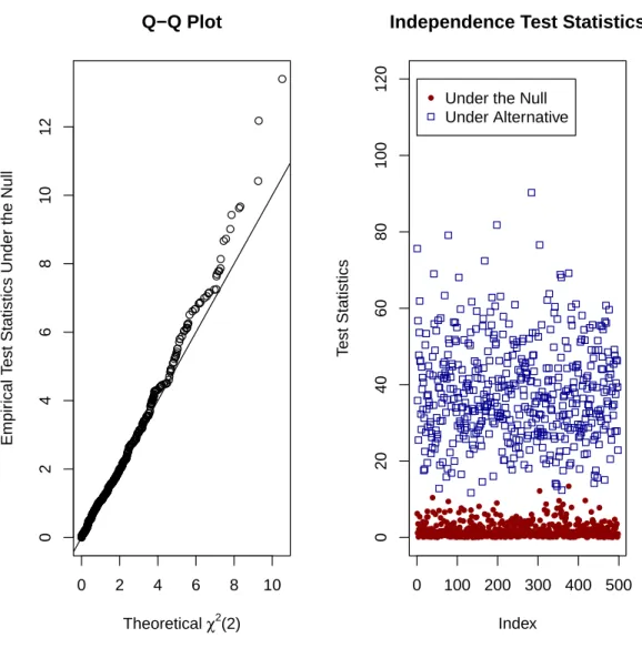
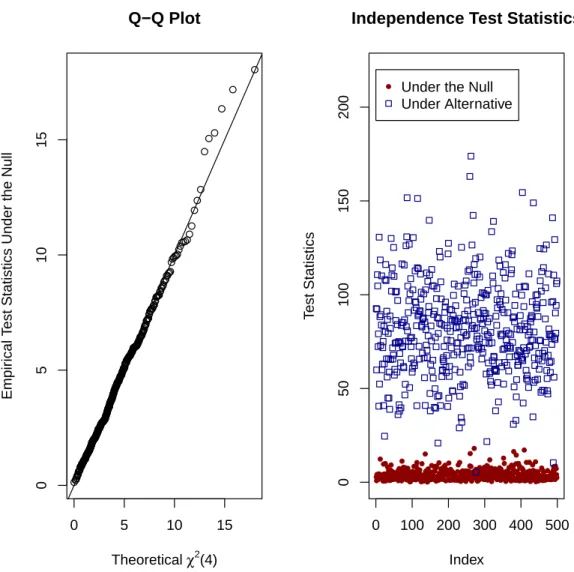
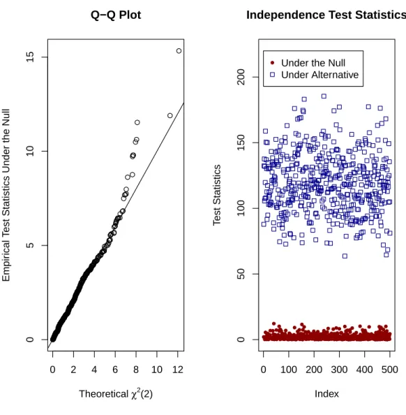
features of propensity score adjustment approach for confounding adjustment, we pro-pose a generalized mixed effect propensity score model to deal with the heterogeneity in treatment assignment process. Few current literatures deal with the random effects in logistic regression model (e.g., Thoemmes and West 2011) for propensity score esti-mation. However, a critical assumption made for the conventional mixed effects model is that the cluster effect term is normally distributed which may be too restrictive for real world medical record data. The validity of this assumption is hard to check for real applications and violation of the assumption will lead to invalid propensity score estimation and result in biased treatment effect estimate. Indeed, the normality as-sumption often does not hold in practice due to many confounding factors and complex heterogeneity involving in the treatment allocation process. To be more flexible in capturing the heterogeneity structure in the treatment allocation process for medical record data, we relax the normality assumption on the random effect in the generalized mixed effects model with an unspecified random effect term. With the PS regression framework, the estimated PS from the proposed model is incorporated to adjust the heterogeneity confounding and obtain the treatment effect estimate that could be bi-ased if the conventional statistical methods are used where the treatment assignment heterogeneity is incorrectly modeled.

Specifically, we consider the following semi-nonparametric (SNP) logistic regression model for the propensity score estimation:

logit(P r(trtij = 1|xij)) =β0+xijβx+ηi (1.12)

Instead of assuming that theηis are normally distributed, we make no specific

assump-tion on the form of the distribuassump-tion of theηis except that it is a smooth density function

(35)

estimated from the above model, then the rest of the analysis will follow the traditional PS regression procedure.

Estimation of propensity score based on the SNP-PS model is challenging. The primary difficulty results from the fact that the likelihood function of model (1.12) is complicated without closed analytic form since it involves the integration over a nonlin-ear integrand. To resolve this problem, various approximation techniques (e.g. Laplace approximation) were developed to avoid the integration (Schall 1991; Breslow and Clay-ton 1993). However, several research (Breslow and Lin 1995; Lin and Breslow 1996) shows that approximations based approaches may yield biased fixed effect estimates, particularly for the binary responses. Alternative approaches (Lee and Nelder 1996; Jiang 1999) were proposed to resolve this difficulty. On the other hand, methods were developed to conduct the integrations via the Markov chain Monte Carlo techniques (Zeger and Karim, 1991) and Monte Carlo EM (MCEM) algorithms (McCulloch 1997; Booth and Hobert 1999). For example, an approach proposed by Booth and Hobert (1999) is based on using rejection sampling technique to generate samples from the appropriate conditional distribution. The advantage of this approach is that it allows to evaluate the Monte Carlo error at each iteration and automatically increase the Monte Carlo sample size accordingly and thus reduce the unnecessary computational workload.

(36)

rejection sampling component may suffer a low acceptance rate in some applications, particularly for binary data when the proportions of 0 and 1 responses within a cluster are severely imbalanced (Chen et al. 2002). To avoid these difficulties, alternatively, we propose a numerical integration approach, i.e. adaptive quadrature integration, to calculate the conditional likelihood for the proposed SNP-PS model (1.12). It can be shown that under the assumption of no other unmeasured confounding covariates, the treatment effect estimate from the proposed SNP-PS framework is unbiased and asymptotic normal.

1.2.3 A Flexible Mixed Effects PS (FM-PS) Model for Clustered Data

When medical record data are multilevel clustered, the robust SNP-PS model pro-posed above is computationally too intensive to be applied to huge multilevel clustered data. More computationally efficient PS models are needed. Note that in the SNP-PS model, the heterogeneity cluster effects are dealt with in the mixed effects PS model which is computationally expensive. Alternatively, we propose a flexible linear mixed effects propensity score (FM-PS) model which does not take into account the hetero-geneity cluster effects in the PS model but instead leaves the heterohetero-geneity adjustment to the subsequent PS covariate adjustment model.

(37)

random cluster effects that the traditional clustered data modeling frameworks made but are generally not held by the real world medical record data. Therefore, the pro-posed FM-PS is not only robust for the random effect density structure due to clustering but also flexible to the correlation between the random effects and other fixed effects confounding covariates. More importantly it is applicable for huge dataset like medical record data for practical use.

As all other propensity score based methods, the standard variance estimation for FM-PS models are not valid either. Accordingly, we propose a cluster bootstrapping procedure to obtain the valid variance estimate empirically.

1.3 Innovation of Proposed Research

1.3.1 Significance of Two-Stage Variance Estimation

(38)

1.3.2 Significance of SNP-PS

The proposed SNP-PS model for dealing with the heterogeneity of treatment al-location provides a uniform approach to adjust the nonparametric heterogeneity con-founding in a robust fashion without the restrictive assumptions. Unlike many existing statistical methods, we extend the prevailing propensity score adjustment approach by including a random effect term without specifying any density distribution in the PS model such that only a simple linear regression is needed to assess the treatment effect. Therefore, SNP-PS is more robust to the distribution misspecification of the random effects.

One challenge with the generalized mixed effects model is that there exists no an-alytic closed form for the log-likelihood function. The double rejection Monte Carlo sampling EM algorithm of Chen et al. (2002) suffers slow convergence and high Monte Carlo errors, which prevents its practical usage for large medical record datasets. Fur-thermore, the double-rejection sampling scheme of Chen et al. (2002) may have low acceptance rate for binary data when the cluster cell size is imbalanced. Alternatively, we propose a computationally efficient numerical integration approach, i.e. adaptive quadrature integration, to avoid the large Monte Carlo errors if the sampling scheme is used and the potential low acceptance rate of the second rejection sampling component.

(39)

on the default variance estimator.

1.3.3 Significance of FM-PS

Medical record data could include hundreds of thousands or even millions of medical records integrated from various resources with the treatments assigned by a number of doctors and patients treated at many different clinics or hospitals. The multilevel clus-tering feature of medical record data further complicates their analysis when treatment effect is intended since it invalidates the crucial independence assumption for the out-comes that many statistical models make. Mixed effects model is the most widely used statistical tool to deal with the clustered and correlated data. However, two impor-tant assumptions for the random effects terms made in the conventional mixed effects models are the independence with respective to other fixed effect terms including the treatment assignment and the normality. These assumptions could be too restrictive for the real world medical record data. We propose a flexible linear mixed effects propen-sity score model to deal with the complicated correlation structures of medical record data conveniently and relax these two assumptions by establishing the equivalence of treatment effect estimates obtained from FM-PS and the dummy variable fixed effects PS (FE-PS) regression model. This equivalence not only relaxes the assumption on the independence between the random effect terms and the fixed effect terms in linear mixed effects model but also the normality assumption for the random effect term.

(40)

score of each cluster in a simple linear mixed effects model without the burdens to model the details of the covariance structure among the random effect and other covariates. Third, FM-PS is computationally efficient as compared to the FE-PS method which is prohibited in the existence of hundreds thousands clusters like many medical record data. Therefore, FM-PS is applicable in practice for the huge clustered dataset. Fourth, a novel cluster bootstrapping procedure to obtain the valid variance estimation for the treatment effect estimate from FM-PS is proposed. Furthermore, a likelihood ratio test statistic is proposed to allow for selecting the efficient and unbiased treatment effect estimate from between FM-PS and SM-PS models.

1.4 Outline of The Remaining of Dissertation

Due to the limitations of existing statistical methods, in this dissertation, new statistical methods are developed for treatment effectiveness inference. The methods focus on addressing some issues of heterogeneity in treatment assignment and multilevel clustering settings for medical record data in comparative effectiveness research. It is the goal to develop robust and efficient statistical methods to deal with these limitations under these scenarios by considering the complicated data structures and relaxing some unrealistic assumptions for real applications. In addition, the statistical properties for the proposed methods and models are extensively explored. Overall, the structure of this dissertation is arranged as the following:

Chapter One: provides the introduction of medical record data, the existing statistical methods for the analysis of these data, and the proposed methods due to the limitations of existing methods.

(41)

studies. The asymptotic results of PS regression models are established in this chapter.

Chapter Three: delineates the details of the proposed semi-nonparametric propensity score (SNP-PS) approach for clustered observational data and its performance under finite sample settings. Practical application of SNP-PS regression method is demon-strated via a real data analysis. In addition, the mathematical derivations for the properties of SNP-PS under large sample scenarios are given in this chapter.

Chapter Four: presents a flexible linear mixed effects propensity score (FM-PS) model for multilevel clustered data. Simulation studies are used to demonstrate FM-PS performance under finite sample setups and different model misspecification settings. Justification for FM-PS approach to model the multilevel clustered data for treatment effectiveness inference is given via cluster bootstrap resampling scheme.

(42)

Chapter 2

A Robust Two-Stage Variance Estimation for PS Regression Analysis

2.1 Introduction

Randomized controlled trial (RCT) is regarded as the gold standard to establish causal effects of drug efficacy. In completely randomized clinical trials, treatments are randomly assigned and the proper randomization procedure guarantees that there exists no systematic difference among subjects for their baseline features in different treatment groups. However, RCTs have their limitations and can not always be con-ducted in practice (e.g. Kramer and Shapiro, 1984; Johnston et al, 2006). Data from observational studies or electronic medical records, on the other hand, are readily avail-able and often used as alternatives for the evaluation of therapy effectiveness and drug efficacy.

(43)

of propensity score (PS) methods are commonly used in practice.

If the multiple regression model is correctly specified, the treatment effect estimator, i.e. least square estimate (LSE), provides the best linear unbiased estimate (BLUE) for the treatment effect, which can be regarded as the benchmark for evaluating the efficacy of different interventions and procedures in comparative effectiveness research. Alternatively, the PS method (Rosenbaum and Rubin 1983) provides a simple and straightforward way to control confounding factors in non-randomized settings. PS methods are increasingly used as alternatives of multiple regression (e.g. Czajka et al. 1992; Schneeweiss et al. 2002; Bang and Robins 2005) due to its simplicity and robust-ness. A propensity score is defined as the conditional probability of a subject being assigned to a particular treatment in a study given a set of observed covariates. Rosen-baum and Rubin (1983) had shown that under certain conditions, the distributions of measured baseline covariates for the treated and untreated subjects are similar condi-tional on any given propensity score. That is, subjects with the same propensity scores, they have the same distributions for the baseline covariates no matter if they come from the treated or untreated groups. They demonstrated that if the treatment assignment is strongly ignorable (i.e. condition (1.3) of Rosenbaum and Rubin, 1983), conditional on propensity scores allows one to obtain an unbiased treatment effect estimate.

(44)

on the PS regression constantly appear in top scientific journals such as JAMA and NEJM (e.g. Koch et al. 2008; Shaw et al. 2008; Eklind-Cervenka et al. 2011; Jackson et al. 2012; Bangalore et al. 2012).

While the PS covariate adjustment provides an efficient and robust treatment effect estimate, the variance estimation of the treatment effect estimate from the standard PS regression model is biased. In practice, researchers routinely base their inference on the default variance estimate from the second stage regression model, ignoring the fact that the PS is a estimated quantity. We recognize that the PS regression approach can be viewed as a two-stage procedure used in a wide class of empirical applications where unobserved regressors, such as expectations, are estimated from an auxiliary statistical model. It is well known that the second-step estimated standard errors and related test statistics based on these procedures are incorrect (Murphy and Topel 1985). In this chapter, we jointly model the distribution of the response and treatment assignment given the propensity scores and develop a simple yet general method for calculating asymptotic standard errors in two-stage models for PS regression analysis. The joint modeling scheme resolves the biased variance estimation issue in the standard PS regression model by taking into account the stochastic errors in the parameter estimates when the propensity scores are estimated.

Similar concerns on the variance estimates have been noticed for other PS-based methods and improved variance estimators have been proposed for PS inverse prob-ability weighting (e.g. Lunceford and Davidian 2004; Williamson et al. 2012), and matching (e.g. Abadie and Imbens 2011). This chapter fills in a gap in variance esti-mation for the PS regression method. Our simulation results further demonstrate the importance of using the proposed two-stage regression model in practical comparative effectiveness research.

(45)

background introductions on existing PS methods. In Section 3, we introduce the PS regression model under the two-stage analysis framework. We then derive the totic result under the proposed two-stage PS regression scheme. Based on the asymp-totic result, we propose a robust and improved variance estimator. In Section 4, we conduct simulations to evaluate the finite sample performance of the proposed variance estimator under various confounding settings and model misspecification scenarios. In addition, to appreciate the usefulness of PS regression method in comparative effec-tiveness research, we compare the performance of our proposed two-stage PS regression method with other existing PS methods, in along with the benchmark method, i.e. multiple regression. We then apply the proposed method to a real data analysis in Sec-tion 5 to demonstrate the practical applicaSec-tion. We end the chapter with discussions in Section 6.

2.2 Existing Methods

We first introduce some notations. Let yi be the response variable, trti be the

binary treatment assignment status (1 for treated and 0 for untreated), andxi be other

observed covariates with dimension ofpfor individuali(i= 1,· · ·, n). The observation for each subject consists of (yi, trti,xi). In this chapter, we focus on the situation where

the response variable is continuous and depends on treatment assignment with effect of αtrt and other observed covariates x:

E(y|trt,x) = α0+αtrt∗trt+x∗αx

Our primary interest is the treatment effect,αtrt, estimate and its variance estimation.

(46)

y(0) are the potential outcomes if the subject had been assigned to the treated and un-treated group, respectively. In reality,y(1) andy(0) can not be observed simultaneously. Instead, they are related to the observed responseyas: y=trt∗y(1) + (1−trt)∗y(0). Under the strongly ignorable treatment assignment assumption of Rosenbaum and Ru-bin (1983), i.e. (y(1), y(0))⊥trt|x, there exist equivalence between ∆ and αtrt which

can be easily checked: αtrt = E(y| trt = 1,x)−E(y |trt = 0,x)⇒ αtrt =E(αtrt) =

E(E(y | trt = 1,x))−E(E(y | trt = 0,x)) = E(E(y(1) | x))−E(E(y(0) | x)) =

E(y(1)|x)−E(y(0)|x) = ∆.

With the strongly ignorable assumption, the confounding factors can be controlled via a simple statistic, i.e. the propensity score (PS). PS is defined as the conditional probability for a unit to receive the treatment given all other observed covariates, i.e.

P Si ≡ P r(trti = 1 | xi). That is, under the strongly ignorable assumption, we have:

(y(1), y(0)) ⊥trt|P S(x) as shown by Rosenbaum and Rubin (1983). In practice, the propensity score is unknown and usually estimated by the logistic regression model:

logit(P S) = xβ. With the parameters β estimated, the propensity score can be esti-mated as:

c

P Si =

exp (xiβ)ˆ

1 + exp (xiβ)ˆ

and the treatment effect can be estimated via PS matching, stratification, IPW, or covariate adjustment.

Under the standard PS regression framework, the treatment effect estimate and its corresponding variance estimation are obtained by fitting the following simple linear regression model:

yi =α0+αtrttrti +α1P Sc_i+_i (2.1)

whereP Sc_iis the estimated propensity scores. We denote the treatment effect estimator

(47)

unbiased under the strongly ignorable and linearity assumptions, the default variance estimate (denoted as V ard( ˆαtrt,P SR)) from the standard PS regression model (2.1) is

biased as will be demonstrated by the extensive simulation studies in Section 2.4.

2.3 Two-Stage Framework for PS Regression

To delineate the proposed variance estimator, we first express the PS regression analysis as a two-stage regression model shown below:

Stage 1 Model: trti |xi ∼f(trti |xi,θ1)

Stage 2 Model: (yi, trti)|P S(xi,θ1)∼f(yi |trti, P S(xi,θ1),θ2)f(trti |P S(xi,θ1))

where θ1 and θ2 are the parameter sets associated with Stage 1 and 2 models. The

unknown PS score,P S(x,θ1)(=P r(trt= 1 |x,θ1)),is a function of x and θ1.

The log-likelihood of Stage 1 model is

l1(θ1) =

n

X

i=1

l1,i(θ1) =

n

X

i=1

logf(trti |xi)

=

n

X

i=1

{trti∗log(P Si) + (1−trti)∗log(1−P Si)} (2.2)

where P Si = P r(trti = 1 | xi,θ1). If the logistic regression model is used in Stage 1

model, then P Si =

exp(β0+xiβ) 1+exp(β0+xiβ)

and θ1 = (β0,β)

0 . The log-likelihood of Stage 2 model is

l2(θ1,θ2) =

n

X

i=1

l2,i(θ1,θ2) =

n

X

i=1

logf(yi, trti |P Si)

=

n

X

i=1

log{f(yi |trti, P Si,θ2)f(trti |P Si)}

=

n

X

i=1

logf(yi |trti, P Si,θ2) +

n

X

i=1

(48)

f(yi | trti, P Si,θ2) = φ(yi;α0+αtrttrti+α1P Si, σ2) where function φ(y;µ, σ2) is the

normal density function with meanµ and variance σ2. Thus, θ2 = (α0, αtrt, α1, σ2)

0 .

In Stage 1 model, the parameter θ1 and PS score, P Si, are first estimated via

equation (2.2) as ˆθ1 =argmax_θ₁l1(θ1) and P Sc_i =P S(x_i,θˆ₁), respectively. Then the

estimated PS scores are plugged into equation (2.3) for estimating θ2, which contains

the treatment effectαtrt, our primary interest. Specifically, in the second stage analysis,

ˆ

θ2 =argmax_θ

2l2(ˆθ1,θ2). Note that when P Sis are replaced by P Scis, maximizing the

likelihoodl2(θ1,θ2) reduces to maximizing the likelihood of the following simple linear

regression model:

yi =α0+αtrttrti+α1P Sc_i+_i,

i.e., the standard PS regression model. We note that the terml1,i(θ1) inl2,i(θ1,θ2) plays

no role in estimating θ2 but it is a critical term for the variance estimation. Ignoring

this term will result in variance estimate very close to the one given by the standard PS regression model (2.1), i.e. V ard( ˆαtrt,P SR), which tends to be biased. We denote the

treatment effect estimator for parameter αtrt as ˆαtrt,P under our proposed two-stage

framework. Under some regularity conditions, we have the following asymptotic results for the treatment effect estimate ˆαtrt,P:

Theorem 2.3.1. The treatment effect estimator αˆtrt,P is asymptotically normally

dis-tributed with,

√

n( ˆαtrt,P −α∗trt)→N(0, σ

2 22)

where σ2

22 is the second diagonal element of the covariance matrix Σ given as the

fol-lowing:

Σ=V2+V2[CV1CT −RV1CT −CV1RT]V2

withV−₁1 =E

∂l1

∂θ1

∂l1

∂θT1

, V−₂1 =E

∂l2

∂θ2

∂l2

∂θT2

,C =E

∂l2

∂θ2

∂l2

∂θT1

(49)

andR=E

∂l2

∂θ2

∂l1

∂θT1

. Under the strongly ignorable condition (1.3) and the

lin-earity assumption in COROLLARY 4.3 of Rosenbaum and Rubin (1983), α∗_trt can be

replaced by αtrt, the true marginal treatment effect.

The proof of Theorem 2.3.1 can be found in Appendix I. The above theorem provides us a basis for a modified variance estimator. To estimate the covariance matrix Σ, we propose a sample estimate ofΣ as the following:

ˆ

Σ= ˆV2+ ˆV2[ ˆCVˆ1Cˆ

T

−RˆVˆ1Cˆ

T

−CˆVˆ1Rˆ

T

] ˆV2

where ˆV−₁1 = 1_nPn i=1

∂l1,i

∂θ1

∂l1,i

∂θT1

|ˆ

θ1

, Vˆ−₂1 = 1_nPn i=1

∂l2,i

∂θ2

∂l2,i

∂θT2

|ˆ

θ1,θˆ2

, Cˆ =

1

n

Pn

i=1

∂l2,i

∂θ2

∂l2,i

∂θT1

|_θˆ

1,θˆ2

and ˆR= _n1Pn

i=1

∂l2,i

∂θ2

∂l1,i

∂θT1

|_θˆ

1,θˆ2

, respectively. Matrix ˆΣ provides a good estimate to Σ as can be demonstrated by the simulation studies below. The proposed variance estimator of the treatment effect estimate ˆαtrt,P is ˆσ222 which is the

second diagonal element of covariance matrix ˆΣ.

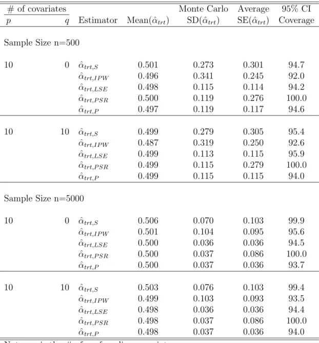
2.4 Simulation Studies

To evaluate the performance of the proposed two-stage regression estimator versus other existing estimators, we conduct simulation studies under various confounding settings as described in the following. Specifically, we compare the treatment effect estimator using the proposed two-stage model, i.e. ˆαtrt,P, versus the estimates from PS

stratification ( ˆαtrt,S), IPW ( ˆαtrt,IP W), multiple regression ( ˆαtrt,LSE), and the standard

PS regression ( ˆαtrt,P SR).

Treatment allocation model: In our first set of simulations, the treatment assign-ment is based on the following mechanism:

(50)

where the confounding covariate vectors x1i = (x1i,1,· · ·,x1i,p)T have p independent

covariates. We let half of the confounding covariates be binary and the other half be continuous. For the binary variables, they follow Bern(0.5) and the continuous variables are simulated fromN(0,1). For the ease of description, we let each parameter

βx,j inβx = (βx,1,· · · , βx,p)

0

be randomly generated fromN(0,1) but they are fixed for all the subsequent simulations.

Data generating model: The responses are generated based on the following data generating process:

yi =αtrttrti+x1iαx+i, (i= 1,· · ·, n) (2.5)

where i ∼ N(0,1) and is independent of trti and x1i. The true treatment effect αtrt

is fixed at 0.5. The effect of each confounding covariate, αx,j (j = 1,· · · , p), is also

generated fromN(0,1).

In observational studies, there may exist many covariates and we may not know which are the true confounding factors and which are not. It is common to include most if not all of them in the analysis. To mimic the real world observational data, in addition to the (true) confounding covariatesx1i, we also simulate an additional set

of q (q ≥ 0) nuisance variables, x2i. Again, among the q nuisance variables, half of

them are generated fromBern(0.5) and the other half follow N(0,1). These nuisance variables have no effects on either the response variabley or the treatment assignment

trt. However, we include the observed covariates xi = (xT1i,xT2i)T in all analysis to

mimic the data analysis in practice. For cases where q= 0, only the true confounding covariates are included, the best scenario that could happen in practice.

(51)

of confounding covariates p and the number of nuisance variables q. For each simu-lation setup, the results are based on 1000 simusimu-lations. Column “Mean( ˆαtrt)”

repre-sents the average treatment effect estimate, column “Monte Carlo SD( ˆαtrt)” shows the

Monte Carlo standard deviation of the treatment effect estimate, and column “Average SE( ˆαtrt)” presents the average standard error for the treatment effect estimate.

Inspecting Table 2.1 reveals that the treatment effect estimate is very close to the true effect size 0.5 in all situations indicating the unbiasedness of treatment effect es-timate under different analysis schemes. The value in column “Monte Carlo SD( ˆαtrt)”

can be viewed as the true error of treatment effect estimate for each estimator. A closer inspection of this column for the first part of Table 2.1 clearly shows that the stan-dard deviations for the LSE, the stanstan-dard PS regression and the proposed two-stage regression are all close to each other. This indicates that the PS regression based treat-ment effect estimators can be almost as efficient as the one from the multiple regression method. A further inspection of this column reveals that both PS stratification and IPW methods provide less efficient estimates.

Most importantly, comparing the column of “Average SE( ˆαtrt)” with the column

of “Monte Carlo SD( ˆαtrt)” for the standard PS regression estimator, i.e. ˆαtrt,P SR, we

(52)

two-stage framework is always very close to the standard deviation in all simulation settings no matter if the sample size is large or not. Furthermore, the corresponding 95% CI coverage for the proposed two-stage estimator, i.e. ˆαtrt,P is close to 95% in all

simulation settings and further confirms the unbiased variance estimation.

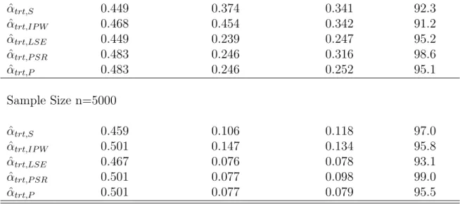
To further investigate the robustness property of the proposed variance estimator, we conducted two additional simulations by varying the data generating model and the treatment allocation model. Specifically, we consider the following two model misspec-ification scenarios:

Misspecification of PS model: we keep the data generating model (2.5) the same but change the treatment assignment from the logistic regression model (2.4) to the following allocation mechanism:

logit{P Si(= P(trti = 1|x1i))}=β0+β1x21i,1+x1iβx

whereβ_x = (βx,1, βx,2,· · · , βx,p)

0

and x1i = (x1i,1, x1i,2,· · ·, x1i,p), respectively. That is,

the first continuous covariates x1i,1s affect the treatment assignment trt both linearly

and quadratically. However, when estimating the propensity scores, we only include the linear terms of all observed covariates xi in our analysis. In this sense, the PS

model is misspecified but not the multiple regression model.

Misspecification of multiple regression model: we keep the treatment allocation mechanism (2.4) but change the data generating model as follows:

yi =αttrti+α1x12i,1+x1iαx+i.

Here αx = (αx,1, αx,2,· · · , αx,p)

0

and x1i = (x1i,1, x1i,2,· · ·, x1i,p), respectively. In this

simulation, the first continuous covariatesx1i,1s affect the responseyi both linearly and

(53)

all observed covariates. That is the multiple regression model is misspecified. However, the PS model is not misspecified. For each of the model misspecification scenario, we consider two sample size scenarios, i.e. 500 and 5,000. The simulation results are presented in Table 2.2.

From the first half of Table 2.2 where the PS model is misfitted, we note that the treatment effect estimates based on different estimators are quite close to the true effect size except the PS stratification estimator. This observation keeps unchanged when the sample size increases from 500 to 5000. It is evident from Table 2.2 that the variance estimation via the standard PS regression is far away from the true variance. However, the variance estimate based on the proposed two-stage method is always close to the true variance.

In the second half of Table 2.2 where one of the covariates affects the response quadratically, we notice that the treatment effect estimates from PS stratification, IPW, and multiple regression methods all suffer biasness. The biasness from IPW gets reduced when the sample size increases while the biasness does not get improved for PS stratification and multiple regression. On the other hand, the treatment effect estimates from the standard PS regression and the proposed two-stage regression framework are unbiased. However, the variance estimation via the standard PS regression is severely upward biased from the true one. In contrast, our proposed method always provides an accurate variance estimate for the true variance.

(54)

is always biased. In contrast, the proposed variance estimation based on the two-stage framework is consistently close to the true variance in all scenarios considered.

2.5 Real Data Analysis

To demonstrate the usage of the proposed method, we applied it to the analysis of a breast cancer study by the German Breast Cancer Study Group (Rauschecker et al. 1995). The study originally was intended as a randomized trial but it had to be changed to an observational study due to the low randomization rate. The primary objective for this study was to compare two breast cancer treatment procedures, i.e. the mastectomy (trt= 0) versus lumpectomy (breast conservation, trt = 1), on the effect of quality of life (QoL) for the breast cancer patients after the surgery. A subset of the data for this study can be obtained from “nonrandom” R package with 646 subjects. The primary outcome was the performance status (PST) 9 months after surgery, which is quantified as a score between 0 and 100 based on the 25 QoL questionnaire responses, where higher scores reflect better QoL. Covariates other than the therapies (i.e. mastectomy vs. lumpectomy) including patient age (Age : ranges from 23 to 82) and tumor size (ts: 1mm ∼ 22mm) are considered as potential confounding factors.

We categorized age as young (age: ≤ 55) and old (age: > 55) and tumor size as small (ts: ≤ 10mm) and large (ts: > 10mm), respectively as did in Senn et al (2007). Distribution of baseline characteristics for these two covariates among the two treatment groups and each stratum of age and tumor size combination are given in Table 2.3.

(55)

patients with larger tumor size prefer lumpectomy procedure. This suggests that the interaction of age and tumor size plays a role on the treatment assignment process. Thus, we use the following logistic regression model to estimate the propensity score:

logit{P Si(=P r(trti = 1|(agei, tsi)))}=β0+β1∗agei+β2∗tsi+β3∗agei∗tsi

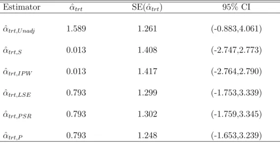
Analysis results using different analysis schemes are presented in Table 2.4.

First row of Table 2.4 presents the crude treatment effect estimate of 1.589 without adjusting any confounding covariate. However, after adjusting the confounding factors, the standard PS covariate adjustment, the proposed two-stage framework, and the mul-tiple regression all end up with a sharply reduced treatment effect estimate as 0.793. The treatment effect estimates using the PS stratification (with 4 strata) and IPW scheme are even more sharply reduced to 0.013. All methods give us positive treat-ment effect estimate indicating that the QoL for patients in the breast conservation group is better than that of mastectomy group. However, this conclusion is not statis-tically significant which can be easily checked from the corresponding 95% confidence intervals. A further inspection of the standard error from each confounding adjustment scheme also reveals that the standard error based on the proposed two-stage regression framework is the smallest one among all methods compared.

2.6 Discussion

(56)

variance estimator was proposed based on the asymptotic result. As shown by our simulations, the variance estimator from the standard PS regression model is biased in general and this will lead to dramatically reduced power for hypothesis testings. This variance estimator did not take into consideration the fact that the PSs used in the second stage regression were estimated with errors. In contrast, the proposed two-stage regression framework took this into consideration and provided an accurate variance estimate.

(57)

Table 2.1: Simulation Results Under Settings (2.4) & (2.5)

# of covariates Monte Carlo Average 95% CI

p q Estimator Mean( ˆαtrt) SD( ˆαtrt) SE( ˆαtrt) Coverage

Sample Size n=500

10 0 αˆtrt,S 0.501 0.273 0.301 94.7

ˆ

αtrt,IP W 0.496 0.341 0.245 92.0

ˆ

αtrt,LSE 0.498 0.115 0.114 94.2

ˆ

αtrt,P SR 0.500 0.119 0.276 100.0