B
ANKC
APITALR
EGULATION ANDS
YSTEMICR
ISK IN THEP
RESENCE OFE
NDOGENOUSF
IRES
ALESSamuel Rosen
A dissertation submitted to the faculty of the University of North Carolina at Chapel Hill in par-tial fulfillment of the requirements for the degree of Doctor of Philosophy in the Department of
Finance at the Kenan-Flagler Business School.
Chapel Hill 2018
Approved by:
Mariano M. Croce
Yasser Boualam
Itay Goldstein
Yunzhi Hu
c
2018
ABSTRACT
SAMUEL ROSEN: Bank Capital Regulation and Systemic Risk in the Presence of Endogenous Fire Sales.
(Under the direction of Mariano M. Croce)
In a model with heterogeneous banks and endogenous fire sales, the tightening of bank capital
regulation can aggravate fire sales, leading to larger bank losses and higher systemic risk. When
calibrated to the data, the least costly policies to mitigate systemic risk raise both ex ante capital
requirements and ex post shortfall penalties. These policies also assign relatively higher capital
requirements to banks that can better offset price declines during a fire sale, consistent with the
recently implemented capital surcharge for global systemically important banks (G-SIBs). My
findings provide further support for leading-edge macroprudential tools, including stress tests and
ACKNOWLEDGMENTS
I am extremely grateful to Yasser Boualam, Max Croce, Itay Goldstein, Yunzhi Hu, and
Chris-tian Lundblad for their guidance and support. I also thank Sirio Aramonte, Anna Cororaton, Jesse
Davis, Deeksha Gupta, Mohammad Jahan-Parvar, and John Schindler for their valuable comments
and feedback. Financial support from the Royster Society of Fellows (UNC) and the Macro
Fi-nancial Modeling Group (Becker Friedman Institute at the University of Chicago) is gratefully
acknowledged.
I also need to thank my family for their love, support, and everything else they have done to
help me get to where I am today. I could not have done it without them. First and foremost, I thank
my beautiful wife Eileen for supporting me through the PhD program, listening to my practice
presentations, reading my drafts, bringing me Taco Bell in between my AFA interviews, and, in
general, for putting up with my nonsense. I thank my best big brother Josh for his hospitality and
for being able to see the rockets coming, which most people never do. I thank my parents for
providing me with all of the best educational opportunities and for encouraging me to pursue my
dreams. And finally, I thank the whole Hou family for believing in me from day one and honoring
TABLE OF CONTENTS
LIST OF TABLES . . . vii
LIST OF FIGURES . . . viii
1 Introduction . . . 1
2 A Model of the Cross Section of Banks . . . 7
2.1 Setup . . . 7
2.2 Equilibrium and Optimality Conditions . . . 17
2.3 Systemic Risk . . . 20
2.4 Endogenous Fire Sale Channel . . . 22
3 Quantitative Policy Analysis . . . 24
3.1 Stylized Facts and Calibration . . . 24
3.2 Increasing Ex Post Penalties and Capital Requirements . . . 31
3.3 Policies To Mitigate Systemic Risk . . . 35
4 Relation to Current Regulatory Policy . . . 41
4.1 Capital Requirements . . . 41
4.2 Ex Post Penalty . . . 42
4.3 Regulatory Stress Tests . . . 43
4.4 Countercyclical Capital Buffer . . . 45
4.5 Liquidity Requirements . . . 46
5 Conclusion . . . 48
A Proofs . . . 50
C Data Details . . . 68
C.1 Bank Sample Construction . . . 68
C.2 Key Variables Within FR Y-9C Dataset . . . 69
C.3 Constructing Time Series of Holdings for Security Types . . . 69
C.4 Computing Share Sold and Unrealized Losses . . . 71
D Calibration Details . . . 73
D.1 Parameters Directly Measured in the Data . . . 73
D.2 Parameters Chosen to Match Initial Portfolio Shares and Selling Decisions . . . . 76
D.3 Increasing Capital Requirements and Equity Capital . . . 77
LIST OF TABLES
3.1 Aggregate Banking Sector Securities Portfolio in 2008Q4 . . . 26
3.2 Parameters Directly Measured in the Data . . . 29
3.3 Parameters Chosen to Match the Data . . . 30
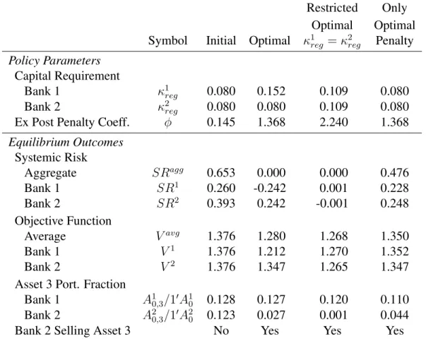
3.4 Optimal Policy to Mitigate Systemic Risk . . . 37
C.1 Constructing Securities Holdings from FR Y-9C Data . . . 70
LIST OF FIGURES
2.1 Model Timeline . . . 8
2.2 Example Optimal Asset 3 Selling Function . . . 20
3.1 Return Indices for Various Security Types 2008Q1-2009Q1 . . . 25
3.2 Risky Security Selling and Market-Based Capital Ratios during 2008Q4 by BHC Asset Size . . . 27
3.3 Effect of Increasing the Ex Post Penalty Parameter (φ) . . . 32
3.4 Effect of Increasing Capital Requirements (κ1 regandκ2reg) . . . 34
3.5 Optimal Policies for Different Cross Sections . . . 40
D.1 Aggregate Net Charge-Off Rates . . . 74
D.2 Tier 1 Capital Ratios by BHC Size Group . . . 78
CHAPTER 1
INTRODUCTION
In my dissertation, I investigate the channels through which tighter bank capital regulation
affects the real costs of a financial crisis when fire sales are determined endogenously. The
motiva-tion for this topic is twofold. First, regulators responded to the financial crisis of 2007–2009 with
the “most significant reregulation of the banking industry since Glass-Steagall.”1 These reforms
are intended to reduce the severity of the next financial crisis, and many involve tighter
regula-tion of bank capital. Second, many papers document and argue that fire sales are an important
contributor to the severity of a financial crisis through their ability to propagate losses throughout
the financial system (Brunnermeier 2009; Hanson, Kashyap, and Stein 2011; Shleifer and Vishny
2011; Duarte and Eisenbach 2015). However, no paper to my knowledge has modeled the
inter-play between capital regulation and fire sales. The main contribution of this paper is to show the
significant impact of this connection for policy analysis.
In the first step of my analysis, I develop a three-period model with heterogeneous banks and a
regulator. Banks choose their asset portfolios anticipating a potential crisis. Conditional upon the
crisis state, banks may choose to sell assets. These selling decisions can cause market prices to
decline because of limited potential buyers, and I refer to this outcome as a fire sale. The severity of
the fire sale is endogenous because it depends on the volume sold. Banks are heterogeneous in their
ability to liquidate assets during a crisis, which affects both optimal portfolio and selling decisions.
As a result, the cross section of banks is a key input in determining equilibrium outcomes.
The regulator can influence bank behavior through two capital-based policy tools: ex ante
1A description of the Dodd-Frank Wall Street Reform and Consumer Protection Act of 2010 from a February 13,
capital requirements and an ex post penalty. The ex post penalty is increasing function of the
amount by which a bank violates its requirement, commonly known as its capital “shortfall.” The
regulator’s objective is to reduce systemic risk, which is a measure that indirectly captures the real
costs of a crisis. I define systemic risk according to the level of aggregate equity capital in the
banking sector during a crisis state.2 Through its capital-based tools, the regulator can ensure that
aggregate bank capital remains high during a crisis and therefore reduce systemic risk.
In the second step, I calibrate the model using data from regulatory filings and perform
quan-titative policy analysis. As part of this process, I also document novel stylized facts about banks’
selling behavior during the financial crisis. Using the calibrated model, I assess the effects from
tightening regulatory parameters and solve for the least costly policies to mitigate systemic risk.
The key mechanism behind my results is found in the optimal selling decision of a bank. When
a bank sells an asset in a fire sale, it incurs a realized loss. This loss occurs because the bank is selling while the price declines, so it effectively sells at a weighted average price between the
asset’s initial and fire sale values. If a bank does not sell an asset that experiences a price decline,
it incurs anunrealizedloss from marking down the value on its balance sheet (i.e., mark-to-market accounting). There is a benefit to selling while the asset price is declining, because a realized loss is
necessarily smaller than an unrealized loss. A bank optimally decides to sell if this opportunity to
minimize the loss is large enough. Many factors affect the size of this benefit, including regulation
and the specific weighted average price at which the bank can sell.
My analysis delivers three main results. First, I show the existence of an endogenous fire
sale channel through which tighter capital regulation can unintentionally lead to higher systemic
risk. Undercapitalized banks sell securities to improve their capital ratio in order to reduce ex
post shortfall penalties. Tighter regulation effectively increases this benefit and therefore makes
the decision to sell more attractive, all else held equal. If more banks sell, the fire sale externality
sharpens, and system-wide losses increase. For this endogenous fire sale channel to materialize,
2Researchers have proposed many alternative definitions and measures for systemic risk, and currently there is no
the probability of a crisis must be sufficiently small so that banks do not hold a capital buffer to
avoid selling assets.
Second, in my quantitative analysis, I show that the least costly policies to mitigate systemic
risk raise both ex ante capital requirements and ex post shortfall penalties. This result highlights
that these regulatory tools provide systemic risk reduction with different cost-benefit tradeoffs.
Capital requirements are costly to banks because they are applied ex ante and force a bank to
hold additional capital in both noncrisis and crisis states of the world. Ex post penalties, on the
other hand, are generally less costly to banks because the penalty is only applied in the crisis
state (i.e., the penalty is state contingent). However, banks find it increasingly expensive to adjust
their portfolios in response to larger penalties. As a result, raising capital requirements eventually
becomes the less costly option for achieving further systemic risk reduction.
Third, these least costly risk-mitigation policies assign relatively higher capital requirements
to banks that can better offset price declines during a fire sale. This “capital surcharge,” which
is 6% to 8% depending on parameter assumptions, is the result of bank heterogeneity and the
regulator’s objective. I assume banks fundamentally differ in the effective price they receive when
selling during a fire sale, an assumption motivated by the data and empirical evidence from the
literature. Banks that can sell at a lower discount can generally be described as better able to offset
price declines. A simpler and more specific interpretation is that some banks can sell faster during
periods of rapid price decline. “Slow” banks incur larger realized losses when selling. As a result,
a higher ex post shortfall penalty is more costly to these banks. Therefore, in order to make up for
the disparity in costliness from increasing the ex post penalty, the regulator optimally raises capital
requirements only for “fast” banks. Intuitively, this capital surcharge compensates for the fact that,
through their selling behavior, “fast” banks impose losses on other banks by causing larger price
declines while incurring smaller realized losses themselves.
My findings have two broad implications for current and future regulatory policy. First, my
quantitative results are consistent with the recently implemented enhanced prudential standards
for institutions deemed “systemically important” and, in particular, the capital surcharge for the
calibration, which are assigned higher capital requirements under the least costly policies.
There-fore, my results provide a fire-sale-based justification for the current regulatory regime. Second,
my findings provide further support for leading-edge macroprudential tools, including stress tests
and countercyclical capital buffers (CCyBs). Their key potential advantage is to reduce systemic
risk without triggering the endogenous fire sale channel.
The model in this paper is closely related to the recent literature that seeks to measure systemic
risk generated through fire sales (sometimes denoted “indirect contagion”). Greenwood, Landier,
and Thesmar (2015) (henceforth GLT) describe a framework in which the effects from an initial
shock can be traced throughout the banking system in terms of selling that both generates and
amplifies losses. Cont and Schaanning (2017) modify the GLT framework to feature asymmetric
selling. They argue that fire sales arise only when one-sided portfolio constraints are breached
as a result of large portfolio losses, which implies an asymmetric reaction of banks to gains and
losses. These models, however, differ from mine along two relevant dimensions: they assume that
asset portfolios are exogenous and also that banks follow prespecified rules in making their selling
decisions. Building upon a similar fire sale framework, I endogenize both the ex ante portfolio
choice and distressed selling decision. After doing so, the connection between policy and systemic
risk becomes clear.
My paper is also related to the theoretical literature that analyzes endogenous fire sales in the
banking sector (e.g., Allen and Gale 2004; Acharya, Shin, and Yorulmazer 2011). As a particularly
relevant example, Diamond and Rajan (2011) develop a model in which fire sales in a future period
are exacerbated because of the risk-shifting incentives at troubled banks in the initial period. My
endogenous fire sale channel result is similar in that the private incentives and decisions of banks
lead to a negative externality via larger fire sale losses. However, my result differs in that selling
decisions do not rely on banks’ limited liability and risk shifting. Instead, the banks sell according
to a cost-benefit analysis influenced by regulatory parameters. Also, unlike Diamond and Rajan
(2011), my model features endogenous portfolio choice and ex ante capital regulation.
of both identifying regulation as the cause of selling and demonstrating a fire sale. Boyson,
Hel-wege, and Jindra (2014) do not find evidence that commercial banks sell affected assets at fire sale
prices during crisis periods. This lack of evidence, however, may be due to data limitations. Other
studies focus on the insurance sector for which the data quality is high and institutional details can
be exploited to make causal inference (Ellul, Jotikasthira, and Lundblad 2011; Merrill, Nadauld,
Sherlund, and Stulz 2014). These papers convincingly demonstrate that the violation of regulatory
constraints causes selling that can generate significant price distortions.
More broadly, the present study contributes to the literature on the role of bank capital
reg-ulation (see Thakor (2014) for a survey). The basic idea is that bank capital affects both risk
management and the ability to withstand economic shocks. However, forcing banks to hold more
regulatory capital may also create costs due to reductions in valuable maturity transformation, the
supply of deposits as safe liquid assets (Gorton and Pennacchi 1990), and/or monitoring from debt
holders (Diamond and Rajan 2001). The optimal capital structure will in theory trade off these
ben-efits and costs. My model, in which the losses from fire sales are a function of the cross section of
banks, provides a richer setting for policy analysis that seeks to determine sufficient levels of bank
capital to mitigate negative real externalities during a financial crisis (i.e., systemic risk). A full
welfare analysis, however, is beyond the scope of this paper, given my reduced-form representation
of agents outside of the banking sector.
The policy analysis in this study contributes to the broader literature analyzing regulatory
pol-icy to address systemic risk (e.g., Allen and Gale 1998; Davila and Korinek 2017; Diamond and
Dybvig 1983; Farhi and Tirole 2012; Lorenzoni 2008; Stein 2012). My results are consistent with
those of Acharya, Pedersen, Philippon, and Richardson (2017), who find that institutions should
be taxed according to the systemic risk they generate. The contribution of this study is to identify
a specific mechanism through which banks actually create systemic risk, thereby delivering an
im-plementation strategy based on available regulatory tools. Further, I specify the characteristic that
leads these banks to generate more risk in the first place: their greater ability to offset price impact.
Finally, this study is related to the literature that explores why profit-maximizing banks choose
of central bank policy and strategic complementarities lead banks to optimally choose correlated
portfolios. Their model, however, does not offer a specific mechanism explaining how banks are
able to coordinate failure in the same states of the world. Allen, Babus, and Carletti (2012) motivate
asset commonality in a network model as a means to reduce the costs of debt, and Acharya and
Yorulmazer (2008) suggest that “herding” is a way to minimize the information spillover from
bad news about other banks. My model provides a distinct channel through which downside risk
materializes (i.e., the fire sale channel) that is consistent with profit-maximizing behavior.
The remainder of my dissertation is organized as follows. Chapter 2 describes the model and
the main theoretical results. Chapter 3 presents the quantitative policy analysis. Chapter 4 relates
CHAPTER 2
A MODEL OF THE CROSS SECTION OF BANKS
I consider a stylized model of the banking sector in order to highlight the interaction between
portfolio choice, capital regulation, fire sales, and systemic risk. After describing the setup, I
char-acterize the equilibrium and select optimality conditions. I then relate these results to equilibrium
systemic risk, focusing on the endogenous fire sale channel described in the introduction.
2.1 Setup
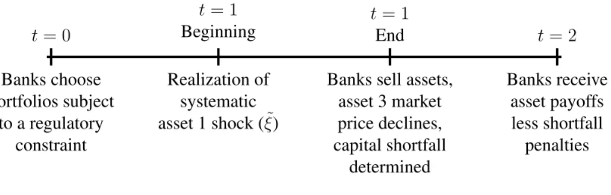
The model features three periods (t= 0,1,2)and an arbitrary number of banks (B). Att = 0, each bank chooses a portfolio from among three risky assets subject to a regulatory capital
constraint. Att = 1, there is a systematic asset shock and the banks may choose to sell assets. These selling decisions can lead to market price declines, which create additional losses for banks
holding the affected assets. The equity capital of each bank is affected by the shock, the bank’s
own selling decisions, and losses due to market price declines. As a result, the bank’s capital ratio
may fall below the regulatory minimum. In such a case, the bank is considered “undercapitalized”
and, equivalently, it has a positive “capital shortfall.” At t = 2, the stochastic payoffs from the risky assets are realized and the bank pays a penalty according to its level of capital shortfall at the
end of the previous period. This setup is summarized in a timeline in figure 2.1.
Three Risky Assets. Banks can choose from among three risky assets for their portfolios. These assets broadly represent the types of risky financial assets that comprise the majority of bank
bal-ance sheets in the data.
1. Asset 1 is an illiquid two-period investment (e.g., bank loans) subject to a systematic shock
att = 1, which is described further below.
Banks choose portfolios subject
to a regulatory constraint
t= 0
Realization of systematic asset 1 shock (ξ˜)
t= 1
Beginning
Banks sell assets, asset 3 market price declines, capital shortfall
determined
t= 1
End
Banks receive asset payoffs less shortfall
penalties
t= 2
Figure 2.1: Model Timeline
3. Asset 3 is a marketable security with downside fire sale risk (e.g., asset-backed securities).
The downside fire sale risk refers to a potential market price decline att= 1that occurs due to aggregate selling.
The asset payoffs at t = 2are determined by a stochastic gross return vector R˜A ∼ (µ,Σ). The
elements of the mean return vector µ and covariance matrix Σ represent the fundamental (i.e., primitive) riskiness of the assets.
Bank Portfolio Problem. At t = 0, bankb is endowed with a fixed amount of equity capital
E0b. Given a cost of debt (RD) and a regulatory framework κbreg, φ, w
, the bank chooses a
vector of asset holdings Ab0, a capital buffer βb, and an amount of borrowing Db0to maximize a mean-variance objective function. Formally, the bank solves the following problem:
max A0,βb,Db0
E0
h
˜
RbEi− γ
2V ar0
h
˜
RbEi (2.1)
subject to
Eb
0 w0Ab
0
=κbreg 1 +βb (2.2)
Db0 = 10Ab0−E0b (2.3)
as well as non-negativity constraints for the choice variablesAb0, βb, Db0 .
problem of a financial institution choosing among multiple assets (e.g., Hart and Jaffee 1974; Kim
and Santomero 1988; Rochet 1992; Calomiris 2009; Glasserman and Kang 2014; Haddad and
Sraer 2015). These preferences capture, in reduced form, a bank’s concern for risk unrelated to
regulation. The mean-variance setup also has intuitive appeal because it is essentially the same as
imposing a value-at-risk (VaR) constraint on the bank’s portfolio. VaR is a common tool used in
practice both internally and by regulators for monitoring the riskiness of bank portfolios.
Equation (2.2) represents the regulatory capital requirement constraint. Given equity capital
E0b, a bank’s portfolio and borrowing choices must result in a capital ratio that is greater than or equal to the minimum level specified by the regulator (κbreg). This required level can be bank specific. The vectorwcontains risk weights for each asset that are used to compute risk-weighted assets (w0Ab
0), the denominator in the bank’s capital ratio. In practice, risk weights are intended to
align a bank’s capital cushion to the riskiness of its assets, and the specific weight values are
deter-mined by the regulator. The constraint in (2.2) holds with equality because of the non-negativity
constraint for the bank’s capital buffer choice βb
.
The level of borrowing in (2.3) is determined by the bank’s portfolio and buffer choices Ab0 andβb. The debt is to be repaid at t = 2 and the cost of debt(RD)is assumed constant. This modeling
choice has two implications. First, it assumes that debt is not priced according to asset risk, which
is a clear violation of the Modigliani and Miller (1958) conditions. Second, it implies that all bank
debt is long-term, which both is counterfactual and neglects the fundamental aspect of maturity
transformation in banking (Diamond and Dybvig 1983).
I justify the first implication by a combination of deposit insurance and collateralization, both
of which serve to make bank debt information insensitive. Although these elements are not
ex-plicitly included in the model, the literature has long acknowledged these features as common to
and necessary for bank debt.1 Moreover, banking theory often views bank debt as information
1The long-standing justification for deposit insurance is a means to prevent panic-based bank runs (Diamond and
insensitive by design (Diamond 1984).
Despite its long-term appearance, the model still captures the costs associated with short-term
bank debt. The bank pays a penalty att= 2based on its financial distress duringt= 1. In reduced form, this cost represents in part the various costs that a distressed institution may pay when rolling
over short-term debt. This penalty and its interpretation are discussed in greater detail later in this
paper. To summarize, the modeling choice for debt is a simplification that allows me to more easily
focus the analysis on portfolio choice and fire sales but still captures key aspects of bank debt.
The stochastic return on the bank’s equityR˜bEis equal to the gross return on assets still held at the end oft= 1less the cost of remaining debt and penalty costs
˜
RbEE0b ≡R˜0AA˜b1−RDD˜b1−Φ˜
b (2.4)
The quantity values for assets and debt A˜b1andD˜1b are stochastic because they depend on the outcome of an asset shock att= 1. The same is true for the penalty
˜ Φb
.
Bank Heterogeneity. The key heterogeneity across banks is their ability to offset price impact during a fire sale. Specifically, the bank-specific parameter αb determines the price that bank b
receives if it sells during t = 1. As a result, banks can differ in their optimal selling decision even while under the same regulatory framework. Additional consequences are that banks choose
different optimal portfolios at t = 0and changes to regulatory parameters affect bank decisions differently. I discuss the interpretation of this heterogeneity later in this chapter after describing
losses due to fire sales.
Banks may also differ in initial equity capital Eb
0
and minimum regulatory requirement (κb reg).
The former effectively determines the cross-sectional distribution ofαb in the banking sector. The
latter is set by the regulator and therefore is not a fundamental characteristic. However, the
re-quirement level is a significant input into the bank’s optimal decisions.
systematic crisis shock. The distribution of this shock is
˜
ξ =
0 with probability1−q ξ with probabilityq
(2.5)
whereξ ∈(0,1)andq ∈(0,1). The shock is in percentage units and therefore the value of asset 1 holdings for bankbat the end oft= 1is
˜
A1b,1 =1−ξ˜Ab0,1 (2.6)
Equivalently, the bank suffers a proportional loss Ab
0,1ξ
when the crisis state is realized
˜
ξ =ξ.
Selling Assets(s). If the crisis state is realized att= 1, the bank may want to sell its marketable assets. The motivation for doing so is to reduce a penalty that is paid att= 2. Each bankbchooses to sell fractionssb2 ∈ [0,1]and sb3 ∈ [0,1]of its asset 2 and asset 3 holdings, respectively. As a result, its holdings of the marketable assets become
Ab1,2 = (1−sb2)Ab0,2 Ab1,3 = (1−sb3)Ab0,3
Given a realization of the crisis stateξ˜=ξ, each bankboptimally choosessb
2, sb3 to solve
max sb
2∈[0,1],sb3∈[0,1]
E0
h
˜
RbE |ξ˜=ξ
i
− γ
2V ar0
h
˜
RbE |ξ˜=ξ
i
(2.7)
For simplicity, I assume that the bank does not sell in the good state of the world.2
2Technically, a bank would optimally re-optimize its portfolio given the noncrisis stateξ˜= 0. Given the illiquidity
Price Impact from Selling. The volume of selling of asset 3 has an impact on its market price. I denote this price decline in percentage units as Ψ3 ∈ (0,1). The level of the price decline is
determined according to a price impact function in which the only input argument is the aggregate
quantity of asset 3 sold:
Ψ3 ≡Ψ
B
X
b=1 sb3Ab0,3
!
(2.8)
This function satisfies the following general properties:
1. Bounded range: Ψ :R+ →[0,1]
2. Positive price decline requires positive selling:Ψ (0) = 0
3. Monotonicity:Ψ0(·)>0
The form of this price impact follows from the theoretical literature on fire sales, which
charac-terizes fire sales as events in which many potential buyers of an asset are concurrently distressed
(Shleifer and Vishny 2011). As a result, any selling that takes place occurs at a price below the
fundamental value of the asset. The price impact function above represents in reduced form an
outside investor who provides liquidity to the banking sector during a fire sale. As long as this
investor has limited wealth and other investment options, the investor’s demand will be downward
sloping. Equivalently, the offered price is declining in the volume being sold. This exact type of
specification is similarly used in other fire sale frameworks (Greenwood, Landier, and Thesmar
2015; Cont and Schaanning 2017).
Losses Due to Asset 3 Price Decline. Given selling decisionsb3 ∈[0,1]and price declineΨ3 ∈
(0,1), bankbwill incur two types of losses related to asset 3: unrealized and realized. The market value of the remaining asset 3 holdings for bankbis
(1−Ψ3) 1−sb3
Ab0,3 (2.9)
This expression implies anunrealizedloss equal toΨ3 1−sb3
equity capital.3
For the share of asset 3 holdings it sells, bankbreceives
1−αbΨ3
sb3Ab0,3 (2.10)
This expression implies arealizedloss equal toαbΨ3sb3Ab0,3. In other words, the bank receives less
than the amount it paid for the holdings that it sells. Here we see the exact role that the
bank-specific parameterαb ∈(0,1)plays within the model framework. When selling, a bank receives a
weighted average price between the initial and fire sale levels with weights 1−αb, αb
. Ifαb is
close to zero, bankbreceives a high price. Ifαb is close to one, bankbreceives a low price. This
price received directly affects the size of the realized loss. As long asαb <1, the realized loss per
unit sold will always be less than the unrealized loss per unit of asset 3 held.
I follow Cont and Schaanning (2017) in incorporating realized losses and in the way that I
model them (i.e., the α parameter). The authors note that previous studies do not account for the fact that banks liquidate assets at a discount to the current market price, which is known as
“implementation shortfall” in the literature on optimal trade execution (e.g., Almgren and Chriss
2000). Greenwood, Landier, and Thesmar (2015), for example, assume that banks sell at the
current market price and then the market price declines according to a price impact function, which would imply thatαb = 0for all banks. The inclusion of a realized loss, however, is critical
when the decision to sell is endogenous, as in my setup.
A novel feature of my model relative to that of Cont and Schaanning (2017) is that I also allow
3I assume mark-to-market accounting (also known as fair value accounting or FVA) in my setup because of its
banks to be heterogeneous in the α parameter. This type of heterogeneity allows banks to make different optimal selling decisions, all else held equal. I do not explicitly model the underlying
source of this heterogeneity, but there are two broad interpretations. First, some banks may
funda-mentally be able to trade faster, and therefore they receive higher volume-weighted average prices
when selling during periods of price decline. This higher speed may arise from a larger set of
established counterparties or from a larger trading operation within the firm (e.g., a larger number
of traders employed). Second, some banks may have superior information about the direction of
financial markets. Knowing that a large price decline is coming, these banks can begin trading
sooner and therefore will receive a higher volume-weighted average price. These interpretations
are not mutually exclusive, and clearly they imply the same end result. In the quantitative analysis
in chapter 3, I present empirical evidence that banks differ along this dimension.
Summing unrealized and realized, the total losses incurred by bank b due to the asset 3 price decline is
Lb = 1− 1−αbsb3Ψ3Ab0,3 (2.11)
Capital Shortfall Penalty (Φ). A bank pays a penalty att = 2if its capital ratio is lower than the required minimum at the end oft = 1. Specifically, this penalty is an increasing function of the amount by which a bank’s equity capital is below its minimum, which is commonly known as
“capital shortfall.” Capital shortfall at the end oft= 1 (CS1)is defined implicitly
E1+CS1 w0A
1
=κreg (2.12)
whereE1 and w0A1 are the equity capital and risk-weighted asset values, respectively, at the end of t = 1 after all selling activity has concluded. Capital shortfall can be positive or negative. If it is positive, the bank’s capital is below its minimum required level, and the bank is considered
“undercapitalized.”
The penalty that the bank pays att= 2is a linear function of its positive capital shortfall at the end oft= 1:
At t = 0, this quantity is stochastic because it depends on the realization of the asset shock at
t= 1.
This penalty represents all of the costs that a bank’s equity holders should expect to incur if
its capital ratio falls too low. Broadly, these costs come from the regulator, debt holders, and the
issuing of equity. A clear distinction between the costs by source is not important as long as we
assume that the regulator effectively controls the penalty coefficientφ. In chapter 3, I conduct the quantitative policy analysis under this assumption.
The regulatory aspect of this penalty is based on the prompt corrective action (PCA) framework
addressing financial deterioration in banks. This framework describes a sequence of increasingly
stringent interventions dependent primarily upon a bank’s capital ratios. These interventions range
from increased oversight to prohibiting capital distributions to closing and liquidating the bank.4
The goal of PCA is to rehabilitate a bank in order to avoid losses in the FDIC insurance fund, so
these measures are technically not to be viewed as a “penalty” in the punishment sense. However,
from the perspective of equity holders of a bank, PCA measures are effectively a punishment
for becoming distressed. Accordingly, PCA measures were utilized heavily during and after the
financial crisis of 2007–2009.5 Thus PCA resembles quite well the ex post penalty in the model.
The capital shortfall penalty also captures in reduced form the costs that arise from debt holders
in times of distress. Debt-related financial distress costs have been studied extensively in the
literature; these include fundamental-based bank runs (e.g., Allen and Gale 1998), difficulties in
rolling over short-term debt (e.g., Acharya, Gale, and Yorulmazer 2011), and overhang (Admati,
DeMarzo, Hellwig, and Pfleiderer ming). A common feature of these costs is that they are an
increasing function of a bank’s perceived distress level.
Finally, the capital shortfall penalty captures in reduced form the costs of issuing equity (Gomes
4For more details on PCA, see, e.g., the Government Accountability Office report “Bank Regulation: Modified
Prompt Corrective Action Framework Would Improve Effectiveness,” GAO-11-612, Jun 23, 2011.
5Between 2006 and 2010, 569 banks underwent the PCA process and 295 ultimately failed. PCA was implemented
2001). These costs can be viewed as voluntary if the bank chooses to issue equity during or after
the distress period. The costs can also be imposed through formal or informal pressure by the
regulator. As with debt-related costs, any equity-issuance costs would be increasing the level of
bank distress.
Parameter Assumptions. I make the following assumptions about the parameter space to either simplify the analysis or focus on specific outcomes.
Assumption 1 The probability of a crisis (q) is sufficiently small such that no bank holds an excess capital buffer in order to buy fire sale assets.
I describe the “small” condition forq in appendix A. The equilibrium implications from this as-sumption are that banks will either sell asset 3 (s∗3 > 0) or not sell at all (s∗3 = 0) and the outside investor represented by the price impact function is the only buyer. Other papers in the literature
use the expected profit from purchasing assets at fire sale prices as a primary driver in a bank’s
portfolio choice (Allen and Gale 2005; Acharya, Shin, and Yorulmazer 2011), but this type of
story is not the focus of this paper. Instead, by focusing on a crisis for which banks choose not
hold excess liquidity beforehand, my analysis is in the spirit of papers that model liquidity coming
from outside the banking sector (Allen and Gale 1998; Stein 2012).6
Assumption 2 The asset return covariance matrix(Σ)is diagonal.
This assumption greatly simplifies the analytical expressions yet leaves the economics of the
prob-lem unchanged.7
6Allen and Gale (1998) include a large number of wealthy, risk-neutral speculators who hold cash in order to
purchase assets when bank sell off assets cheaply to obtain liquidity. Stein (2012) defines a subset of “patient” investors that both invest in new projects and absorb assets being sold in a crisis state.
7If the true covariance matrix of the asset returnsSis not diagonal, we can perform a Cholesky decomposition (Sis
positive definite because it is a covariance matrix) to findS=LΣL0whereLis a lower triangular matrix andΣis
Assumption 3 The fundamental expected asset return parameters satisfy
µ1 > µ3 > µ2 > RD
This assumption has a few implications. First, in a world with no capital regulation or systematic
shock, a bank would want to hold a positive amount of each asset. Second, it implies that asset 1
earns the highest risk premium and asset 2 earns the smallest risk premium, which is consistent with
the types of real-world assets they represent (bank loans and Treasuries). Third, it guarantees that
banks sell their holdings of asset 3 before selling those of asset 2, which simplifies the presentation
of the optimal selling decision by removing a few special cases (appendix B). This outcome was
also a stylized feature of the data at the height of the financial crisis as shown in chapter 3.
2.2 Equilibrium and Optimality Conditions
Before analyzing the optimal decisions, let us first define an equilibrium.
Definition 1 Equilibrium. An equilibrium is a vector of asset holdings Ab
0
, a capital buffer βb
, a level of debt Db
0
, and a set of distressed selling decisions sb
2, sb3
for each bankbas well as a price decline for asset 3(Ψ3)such that
1. Bank optimality: Ab0, βb, D0b solves thet = 0bankbproblem in (2.1)–(2.3) and sb2, sb3 solves thet= 1bankbproblem in (2.7) given
• Asset 3 price decline(Ψ3)
• Regulatory framework κbreg, φ
• The other model parameters
2. Market clearing: Asset 3 price decline(Ψ3)satisfies
Ψ3 = Ψ
B
X
b=1 sb3Ab0,3
!
Compared to a pure portfolio choice problem (i.e., q = 0), solving this model is significantly more difficult. The asset 3 price decline(Ψ3)is taken as given by each bank att= 0but also must
be consistent with the portfolio choice and selling behavior of all banks at t = 1. However, we gain richness in the model insights because the equilibrium asset 3 price decline(Ψ3)incorporates
the selling behavior of the entire cross section of banks.
The following proposition formalizes the key insight regarding the optimal bank selling
deci-sion:
Proposition 1 Optimal Asset 3 Selling. Ceteris paribus, bankb optimal selling for asset 3 sb
3
is weakly increasing in
• The ex post penalty parameter (φ)
• The minimum capital requirement (κbreg)
• The fire sale price decline(Ψ3)
• The bank’s ability to offset price impact −αb
as long asαb < 1−κb regw3
.
Proof See appendix A.
From a policy perspective, there are two important implications from proposition 1. First,
tightening bank regulation can cause bank b to sell asset 3. This finding is the foundation of the endogenous fire sale channel. Second, banks that can sell at a higher price (i.e., banks that
have a lowα) choose to sell at lower threshold values than other banks, all else held equal. This implication may seem obvious, but it highlights the reason that the cross section of banks is an
important input to both equilibrium outcomes and the choice of the best regulatory policies.
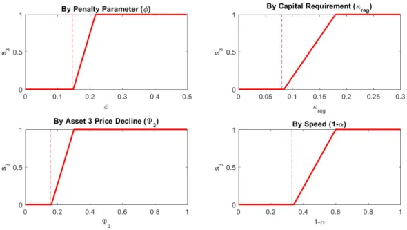
To better understand the optimal selling decision and proposition 1, it is helpful to consider a
policy function is weakly increasing in each panel. The policy functions shown represent a
par-tial equilibrium outcome in which all other inputs (including the equilibrium price Ψ3) are held
constant.
The intuition for this outcome can be understood by comparing the extreme cases in which the
bank sells nothing or everything. If a bank does not sell asset 3 at all(s3 = 0), its payoff att = 2
from asset 3 is a mean-variance payoff less the penalty from the unrealized loss due toΨ3:
(µ3−RD)A0,3−
1
E0 γ
2A
2 0,3σ
2 3
| {z }
Mean-variance payoff
−φ(1−κregw3) Ψ3A0,3
| {z }
Penalty unrealized loss
On the other hand, if a bank sells its entire holding of asset 3 (s3 = 1), its payoff att = 2 from
asset 3 is purely a realized loss due toΨ3
−φ(αΨ3−κregw3)A0,3
| {z }
Penalty realized loss
Combining the expressions yields the net payoff att= 2from selling its entire holdings:
φ
(1−Ψ3)κregw3
| {z }
From reducing assets
+ (1−α) Ψ3
| {z }
Fromα <1
A0,3
| {z }
Benefit from reduced penalty
−
(µ3−RD)A0,3−
1
E0 γ
2A
2 0,3σ
2 3
| {z }
Lost mean-variance payoff
In this expression, we can see that the benefit term is increasing in all of the inputs listed in
propo-sition 1. This benefit comes from two sources. First, selling assets reduces capital shortfall by
reducing assets (the denominator of the capital ratio). As the minimum capital ratio increases
(κreg ↑), the reduction in assets has a larger effect in reducing capital shortfall because of the
lower leverage. Second, realized losses are smaller than unrealized losses for a givenΨ3given that α <1. As the fire sale worsens (Ψ3 ↑), this benefit becomes larger. This benefit is also larger for
Figure 2.2: Example Optimal Asset 3 Selling Function
The underlying parameters are from the calibration in chapter 3 (µ3 = 1.023,RD = 1.0045,w3 = 0.5,α = 0.67, φ = 0.1454,κreg = 0.08, andΨ3 = 0.1558). The dashed lines in each plot indicate the underlying parameter or
equilibrium values, which show that the bank in this example does not sell its asset 3 holdings.
Proposition 2 Capital Buffer. A bank holds zero additional capital buffer if the probability of a crisis (q) is sufficiently small.8
Proof See appendix A.
Absent the ex post shortfall penalty costs, a bank only holds a capital buffer if the asset return
fundamentals are not sufficiently attractive for the capital requirement to bind. Including these
costs, the bank may want to hold an additional capital buffer to reduce the penalties or amount
of selling in the crisis state. Holding such a buffer is costly, however, because the bank gives up
profits in the noncrisis state. The larger the probability of the crisis state (q), the larger the expected benefit from holding a capital buffer. This is the intuition that is formalized in proposition 2.
2.3 Systemic Risk
Following Acharya et al. (2017) and others, I define systemic risk(SRagg)using a measure of
aggregate capital shortfall. This measure captures the relative capitalization of the banking sector
8Whether or not this condition also holds given assumption 1 is difficult to show analytically. Therefore I simply
as a whole. The underlying idea is that aggregate undercapitalization creates negative externalities
in the real economy (e.g., reduced intermediation). Aggregate capital shortfall can be considered
a sufficient statistic for these costs that is relatively easy to compute in practice. As a result, it has
become popular as a measure for systemic risk.
Definition 2 Systemic Risk. Systemic risk is the non-negative amount of aggregate capital short-fall relative to a fixed capital ratio level
SRagg ≡max
( B
X
b=1
SRb,0
)
(2.14)
where each bank’s contribution is defined by
E1b+SRb w0Ab
1
=ζ (2.15)
andζ is the fixed capital ratio level.
Note that, compared to the definition of capital shortfall in (2.12), a bank’s systemic risk
con-tribution is measured relative to a fixed capital ratio levelζinstead of its regulatory minimumκb reg.
For reference, I set ζ = 0.08 in the calibration in the quantitative analysis (chapter 3), which is the value used in theSRISK measure of Brownlees and Engle (2017). This aspect of measuring systemic risk also follows from the literature and explains why increasing capital requirements can
lower systemic risk. Similar to capital shortfall, we can decompose the systemic risk contribution
from any given bankbinto the following three components:
SRb ≈ ξAb0,1
| {z }
Asset 1 Loss
−
Eb
0/(w
0Ab
0)−ζ Eb
0/(w0Ab0)
E0b
| {z }
Initial Capital Ratio Above SR Threshold
+L sb2, sb3;Ab0,Ψ3
| {z }
Net Fire Sale Loss
(2.16)
This decomposition will help us understand the impact from changing policies discussed in chapter
2.4 Endogenous Fire Sale Channel
Using the key results from the model and the definition of systemic risk, I now ready describe
the endogenous fire sale channel. This channel describes a sequence of endogenous effects, starting
with tightening regulation that leads to higher systemic risk. Specifically, tighter regulation can
lead to higher systemic risk through the following sequence:
κbreg, φ ↑=⇒sb3 ↑=⇒Ψ3 ↑=⇒L sb2, sb3;Ab0,Ψ3
| {z }
Net Fire Sale Loss
↑=⇒SRb ↑=⇒SRagg ↑ (2.17)
In the first link, tighter regulation leads bankbto sell asset 3. This effect follows from proposition 1 and requires that bank b was not already selling the asset. In the next link, more selling leads to a larger fire sale price decline, which is a direct result from the properties of the price impact
function in (2.8). In the third link, the larger fire sale price decline leads to larger fire sale losses.
This outcome, which is formally described in the following proposition, occurs as long as the
probability of a crisis (q) is sufficiently small.
Proposition 3 Fire Sale Losses Increasing in Asset 3 Price Decline.Ceteris paribus and assum-ing a positive asset 3 holdassum-ing A∗0,3 >0
, a worsening fire sale(Ψ3 ↑)creates larger bankb fire sale losses if
min
(
µ3−RD 2qφ 1−κb
regw3
,
(1−q) (µ3−RD) +κregw32qφ 2qφαb
)
>Ψ3
Proof See appendix A.
The intuition for proposition 3 is simple: bankb does not shift its ex ante holdings of asset 3 much if the probability of the crisis is low.9 The condition in the proposition guarantees that the
elasticity of a bank’s holding of asset 3 with respect to the fire sale price decline (Ψ3) is less than
one, which implies that total losses (price decline times holding) go up.
9The expression in proposition 3 can alternatively be characterized as holding for a sufficiently small ex post penalty
In the final two links of (2.17), larger fire sale losses lead to larger systemic risk, as defined
above. To summarize, the tightening of bank regulation can lead to more selling, larger fire sale
price declines and losses, and higher systemic risk.
The sequence of effects in (2.17), however, does not describe all of the effects that occur in
equilibrium as the result of tighter capital regulation. There are several other endogenous effects
that occur concurrently, many of which mitigate increases in systemic risk. For example, an
in-crease in capital requirements also forces banks to hold a larger initial capital ratio level. In the
decomposition of systemic risk in (2.16), this effect directly reduces systemic risk.
The ultimate impact on equilibrium systemic risk from changing regulatory parameters
de-pends on the quantitative magnitudes from all effects describe above, and the direction is
diffi-cult to establish analytically. In the next chapter, I explore the equilibrium outcomes from policy
changes numerically in a calibrated model. I also characterize the least costly policies to mitigate
CHAPTER 3
QUANTITATIVE POLICY ANALYSIS
In this chapter, I investigate the quantitative impact from tightening capital regulation, given
parameter values that represent the US banking sector. First, I calibrate the model using asset
holdings data disclosed in regulatory filings. As part of this process, I document novel stylized
facts about asset selling by banks during the financial crisis. Using the calibrated model, I then
assess regulatory policies that mitigate systemic risk under different parameter assumptions and
potential regulatory objective functions.
3.1 Stylized Facts and Calibration
I calibrate the model to both the period before the financial crisis and the observed outcomes
during the financial crisis. The financial crisis offers a relevant empirical example for the model
developed in chapter 2. In particular, the fourth quarter of 2008 resembles the crisis state and
resulting fire sale. During this quarter, large and sharp price declines occurred across many types
of securities, as shown in figure 3.1. The left panel shows return indices for “risky” security types
that experienced steep declines from the beginning of the quarter, while the right panel shows
return indices for “safe” security types that experienced no price declines.
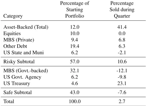
In aggregate, banks were net sellers of risky securities during this period (see table 3.1). Banks
sold 10.6% of their holdings in “risky” securities, while they increased their holdings of “safe”
securities by 7.6% (overall sales of 2.7% of their total securities holdings). A more detailed
break-down of the underlying asset types for the risky and safe subtotals is reported in table 3.1.
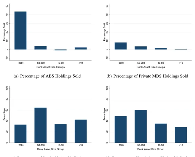
Figure 3.2 shows the share of asset-backed securities and private mortgage-backed securities
sold, by bank asset size groups. I focus on these two types of securities because of their notoriety
during the crisis (Acharya, Cooley, Richardson, and Walter 2009) and because they accounted for
(a) Risky Securities (b) Safe Securities
Figure 3.1: Return Indices for Various Security Types 2008Q1-2009Q1
All indices are computed to have a value of 100 on September 30, 2008. The ABS index is computed from Bloomberg Barclays US Agg ABS Total Return Value Unhedged USD, downloaded from Bloomberg (LUABTRUU Index). The Municipal Bond index is computed from the S&P Municipal Bond Index. IG Corporate is computed from the FINRA Investment Grade Corporate Bond Index. U.S. Treasury values are computed from ICE U.S. Treasury Core Bond TR Index, downloaded from Bloomberg (IDCOTCTR Index). MBS (Govt) is computed from the net asset value of the iShares MBS ETF, which tracks an index composed of investment-grade mortgage-backed pass-through securities issued and/or guaranteed by U.S. government agencies.
the largest banks are the only significant net sellers of asset-backed and private mortgage-backed
securities.
The model suggests a few potential explanations for the cross-sectional difference in selling
behavior. These explanations include differences in (1) the ability to offset price impact αb, (2) the level of distress CS1b, (3) capital requirements (κbreg), and (4) the ex post penalty parameter (φ). Let us consider each of these alternative explanations.
According to market-based capitalization measures, the largest banks faced similar levels of
distress compared to the other size groups. In figure 3.2, I show the relative share of banks and
assets in distress by bank size group. The bottom panels support the conclusion that the largest
banks, as a group, were equivalently undercapitalized according to market-based capital ratios. I
use the market-based measures because they have two advantages relative to the accounting-based
regulatory measures: they are available within the quarter, and they capture changes to the market
value of all assets. In the model, banks have an incentive to sell assets at the beginning of a fire sale
Percentage of Percentage
Starting Sold during
Category Portfolio Quarter
Asset-Backed (Total) 12.0 41.4
Equities 10.0 0.0
MBS (Private) 9.4 6.8
Other Debt 19.4 6.3
US State and Muni 6.2 -2.1
Risky Subtotal 57.0 10.6
MBS (Govt.-backed) 32.1 -12.1
US Govt. Agency 6.2 -9.8
US Treasury 4.6 23.1
Safe Subtotal 43.0 -7.6
Total 100.0 2.7
Table 3.1: Aggregate Banking Sector Securities Portfolio in 2008Q4
Data are from FR Y-9C. Figures used to computed percentage of portfolio are fair value. The classifications into “Risky” and “Safe” are subjective judgments based upon observed price declines during the quarter (see Figure 3.1). Subtotals for percent sold are computed as weighted averages of the share sold for underlying types and cannot be . Wells Fargo and Wachovia are excluded from the computations because of the data issues created by the merger during the quarter. For data details see Appendix C.
that the largest banks did not have a particularly greater incentive to sell during the fourth quarter
of 2008.
The largest banks faced the same regulatory framework (κb
regandφ) as other banks leading up
to the crisis. Even if there were informal differences (e.g., in enforcement), these differences would
not account for the largest banks selling. According to proposition 1, the optimal selling decision
is an increasing function of a bank’s ex ante capital requirement (κbreg) and the ex post penalty parameter (φ). Therefore, the largest banks would be the only group selling only if they hadhigher
values for either parameter. The precrisis evidence does not support this claim. In appendix D.3,
I show that the largest banks had lower capital ratios than most banks. Also, the popular narrative
that large banks were “too big to fail” (Sorkin 2010) implies that, if anything, the largest banks had
(a) Percentage of ABS Holdings Sold (b) Percentage of Private MBS Holdings Sold
(c) Percentage of Banks Under 6% Ratio (d) Percentage of Bank Assets Under 6% Ratio
Figure 3.2: Risky Security Selling and Market-Based Capital Ratios during 2008Q4 by BHC Asset Size
Asset size is total assets in billions of dollars at the beginning of 2008Q4. Wells Fargo and Wachovia are excluded when computing the figures for share sold because of the data issues created by their merger during the quarter. The market-based capital ratio used in the bottom panels is computed as the minimum equity valuation during the quarter divided by risk-weighted assets. The bottom left panel shows the number of banks with ratios below 6% divided by the total number of banks within each asset-size group. The right panel shows the sum of the assets for banks with ratios below 6% divided by the total sum of assets within each asset-size group. For data details, see appendix C.
There is a logical argument based on empirical evidence that may explain why the largest
banks can better offset price impact. These banks have significant broker-dealer subsidiaries and
tend to hold a large percentage of their securities as trading assets1, and these trading businesses
provide advantages during periods of market turmoil. In the context of the corporate bond market,
1The largest banks held 6% to 8% of their securities as trading assets between 2001–2006 compared to approximately
Di Maggio, Kermani, and Song (2017) find empirically that being a central dealer was valuable
between September 2008 and July 2009 in two ways.2 These dealers charged higher prices to
both peripheral dealers and clients, and they also shrank significantly their holdings of bonds that
their clients were selling aggressively. The first finding directly supports a lower value forαb. The
second suggests that these dealers can and do act on private information about market activity from
order flow. This idea is also supported by Barbon, Di Maggio, Franzoni, and Landier (2017), who
find evidence that brokers leak order flow information to their best clients in order to predate on
large liquidations by the other clients. In sum, the advantages from having large dealer subsidiaries
are consistent with better ability to offset price impact (i.e., lowerαb).
Proposition 1 tells us that a bank that is better able to offset price impact (i.e., one with lowαb)
can choose to sell while an otherwise identical bank with a higherαb does not. Therefore, if we
interpret the largest banks as having a lowαb, we can find an equilibrium in which only the largest
banks are selling.
All together, the stylized facts in the data discussed above provide the following implications
for the benchmark model calibration:
1. SetB = 2where bank 1 represents banks over $250 billion in assets as of the beginning of 2008Q4 and bank 2 represents all other banks.
2. The initial equilibrium under pre-2008 regulation must feature only bank 1 selling.
3. Bank 1 can better offset price impact (α1 < α2).
Table 3.2 shows the parameters that I can directly measure in the data. These parameters include,
for example, the return parameters for asset 2, which represents perfectly liquid assets that do not
incur any fire sale discount in the crisis state. Given my distinction between banks 1 and 2, I can
also easily measure the relative size of these banks during the sample period.
2Other over-the-counter markets follow a similar core-periphery structure. Li and Schurhoff (2014) show core dealers
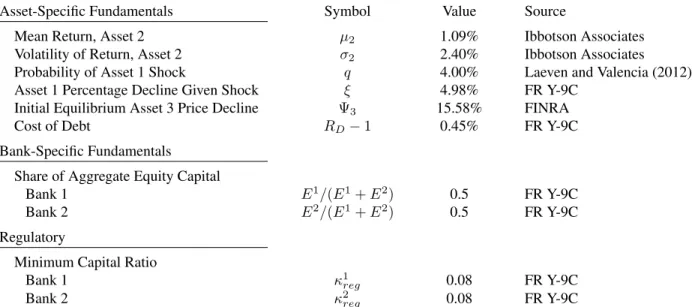
Asset-Specific Fundamentals Symbol Value Source
Mean Return, Asset 2 µ2 1.09% Ibbotson Associates
Volatility of Return, Asset 2 σ2 2.40% Ibbotson Associates
Probability of Asset 1 Shock q 4.00% Laeven and Valencia (2012)
Asset 1 Percentage Decline Given Shock ξ 4.98% FR Y-9C
Initial Equilibrium Asset 3 Price Decline Ψ3 15.58% FINRA
Cost of Debt RD−1 0.45% FR Y-9C
Bank-Specific Fundamentals
Share of Aggregate Equity Capital
Bank 1 E1/(E1+E2) 0.5 FR Y-9C
Bank 2 E2/(E1+E2) 0.5 FR Y-9C
Regulatory
Minimum Capital Ratio
Bank 1 κ1
reg 0.08 FR Y-9C
Bank 2 κ2
reg 0.08 FR Y-9C
Table 3.2: Parameters Directly Measured in the Data
See appendix D for details.
I set the regulatory risk weights (w1, w2, w3) according to the following formula:
wi =
µi−RD
µ1−RD
(3.1)
so that the risk weight values do not distort portfolio outcomes (Kim and Santomero 1988;
Glasser-man and Kang 2014).3
There are several parameters that are either difficult or impossible to measure directly. I choose
these parameters in order to match the observed portfolio holdings and selling decisions (see table
3.3). For banks’ ability to offset price impact (α1 andα2), I solve the model over a range of input
values as a form of sensitivity analysis. Given the crucial nature of these parameters, it is important
to understand how equilibrium outcomes change with cross-sectional heterogeneity.
For the final element of the calibration, I follow Greenwood, Landier, and Thesmar (2015)
and Duarte and Eisenbach (2015) in choosing a linear price impact function for the quantitative
3Other papers find similar results. Rochet (1992) proposes setting risk weights proportional to systematic risk.
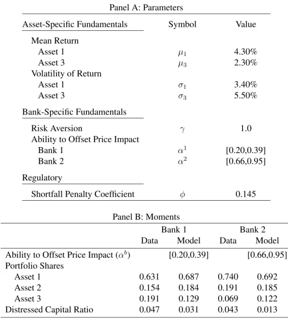
Panel A: Parameters
Asset-Specific Fundamentals Symbol Value
Mean Return
Asset 1 µ1 4.30%
Asset 3 µ3 2.30%
Volatility of Return
Asset 1 σ1 3.40%
Asset 3 σ3 5.50%
Bank-Specific Fundamentals
Risk Aversion γ 1.0
Ability to Offset Price Impact
Bank 1 α1 [0.20,0.39]
Bank 2 α2 [0.66,0.95]
Regulatory
Shortfall Penalty Coefficient φ 0.145
Panel B: Moments
Bank 1 Bank 2
Data Model Data Model
Ability to Offset Price Impact (αb) [0.20,0.39] [0.66,0.95]
Portfolio Shares
Asset 1 0.631 0.687 0.740 0.692
Asset 2 0.154 0.184 0.191 0.185
Asset 3 0.191 0.129 0.069 0.122
Distressed Capital Ratio 0.047 0.031 0.043 0.013
Table 3.3: Parameters Chosen to Match the Data
Forα1andα2, I consider a range of values such thatα1< α2. Data values for portfolio shares are average observed holdings during 2002–2006. Model portfolio shares are averages over theα1, α2 space, but the values do not change much (at most by 0.002). Distressed capital ratios are computed using the minimum market-based capital ratio during 2008Q4. For data details, see appendix C. For calibration details, see appendix D.
exercise:
Ψ B
X
b=1 sb3Ab0,3
!
≡max
(
min
(
ψ3×
B
X
b=1 sb3Ab0,3
!
,1
)
,0
)
(3.2)
The max and min functions ensure that the range of the function is bounded between zero and one.
Otherwise, the basic linear function satisfies all of the price impact function properties described in
chapter 2. In the ensuing quantitative analysis, the equilibrium price decline is never equal to one.
price decline (Ψ3) equal to the value specified in table 3.2.4
In the bottom panel of table 3.3, I compare benchmark calibration model outcomes against
the data. I am able to qualitatively match the data values insofar as they differ across banks. For
example, the model results show that bank 1 holds a smaller percentage of its portfolio in asset 1
and experiences less market-based capital shortfall during the fire sale period.
3.2 Increasing Ex Post Penalties and Capital Requirements
Given a calibration, we can begin our steps toward policy analysis. In this section, I investigate
the effect of tightening each policy tool used in capital regulation, ex post shortfall penalties and ex
ante requirements, one at a time. The goal is to understand the impact from each type of policy tool
and how they may differ. These insights will be helpful in understanding the policies that combine
both.
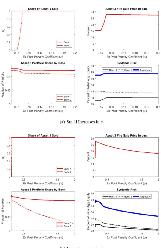
Figure 3.3(a) shows the effects from relatively small increases in the ex post penalty parameter
(φ). Consistent with proposition 1, bank 2 joins the fire sale. As a result, there is a jump in the asset 3 fire sale price decline, and both banks shift their portfolios away from asset 3. Since the
probabiliy of a crisis is only 4%, the portfolio rebalance is modest. Importantly, systemic risk
actually increases over this interval for the penalty parameter because the endogenous fire sale
channel described in section 2.4 dominates.
Figure 3.3(b) highlights the positive effects from increasing the ex post penalty parameter.
Fur-ther increases in this penalty parameter steadily lower the fire sale price decline, as both banks shift
their portfolios away from asset 3. Bank 2 shifts its holdings more dramatically because this bank
suffers larger realized losses during the fire sale episode given its lesser ability to offset the price
impact (highα). As a result, bank 2 is more affected by the increasing ex post penalty parameter. Systemic risk also steadily declines following the initial increase. Based on this outcome, a
regu-lator with the goal of reducing systemic risk should either leave the ex post penalty unchanged or
increase it significantly to take advantage of its positive effect.
Before discussing increasing capital requirements κb reg
, I must clarify an important aspect of
4The expression isψ3= Ψ3/PB
b=1s∗ b 3 A∗
b 0,3
(a) Small Increases inφ
(b) Large Increases inφ
Figure 3.3: Effect of Increasing the Ex Post Penalty Parameter (φ)
this exercise. Technically, banks can meet a higher capital requirement in two ways: by raising
more equity capital (E0b) or by reducing risk-weighted assets (w0Ab0). In order to preserve the size distribution of the banks and the size of the banking sector, I adjust equity capital (Eb
0) in step with
capital requirements (κb
reg). A benefit to this approach is that systemic risk does not mechanically
shrink, because banks become smaller with rising capital requirements. See appendix D.3 for
implementation details and recent empirical evidence.
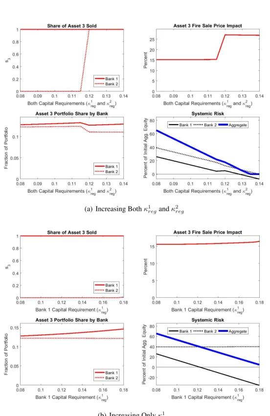
In figure 3.4(a), I show the effect of increasing capital requirements for both banks κ1
reg, κ2reg
.
In the top left panel, we see that bank 2 switches to selling asset 3 after its capital requirement is
raised above 11%, which is an expected outcome based on proposition 1. As a result, the fire sale
price decline of asset 3 jumps up and both banks shift their portfolios away from asset 3. In the
bottom right panel, we see that, for each bank, contributions to systemic risk are monotonically
decreasing, except for the slight uptick to bank 1 when bank 2 switches to selling. Note, however,
that systemic risk still declines in aggregate, so the endogenous fire sale channel does not dominate
in this instance.
The key difference in the effects from increasing capital requirements versus increasing the
ex post penalty parameter can be explained through the decomposition of a bank’s contribution to
systemic risk in (2.16). Increasing the capital requirement effectively forces a bank to hold a larger
initial capital ratio level relative to the systemic risk threshold (ζ). Therefore the bank’s systemic risk contribution mechanically declines, all else held equal. Systemic risk contributions can even
turn negative, which means that a bank’s distressed capital ratio level is above the systemic risk
threshold (ζ) at the end of the fire sale period. This benefical effect differs from the portfolio reallocation caused by increasing the ex post penalty parameter (figure 3.3(b)), as the reallocation
effect lowers the net fire sale loss component of a bank’s systemic risk contribution.
If the regulator only increases the capital requirement for bank 1 (κ1reg), bank 2 does not switch to selling asset 3. This result is shown in figure 3.4(b). This outcome should be expected, as
propo-sition 1 tells us that a bank’s optimal selling function is increasing in its own capital requirement,
not the requirements of other banks. As a related outcome, the bottom right panel shows that the
(a) Increasing Bothκ1regandκ2reg
(b) Increasing Onlyκ1reg
Figure 3.4: Effect of Increasing Capital Requirements (κ1reg andκ2reg)