A behavioral design flow for synthesis and optimization of asynchronous systems

(1)

A Behavioral Design Flow for Synthesis and

Optimization of Asynchronous Systems

John B. Hansen

A dissertation submitted to the faculty of the University of North Carolina at Chapel Hill in partial fulfillment of the requirements for the degree of Doctor of Philosophy in the Department of Computer Science.

Chapel Hill 2012

(2)

(3)

ABSTRACT

JOHN B. HANSEN: A Behavioral Design Flow for Synthesis and Optimization of Asynchronous Systems.

(Under the direction of Montek Singh.)

Asynchronous or clockless design is believed to hold the promise of alleviating many of the challenges currently facing microelectronic design. Distributing a high-speed clock signal across an entire chip is an increasing challenge, particularly as the number of transistors on chip continues to rise. With increasing heterogeneity in massively multi-core processors, the top-level system integration is already elastic in nature. Future computing technologies (e.g., nano, quantum, etc.) are expected to have unpredictable timing as well. Therefore, asynchronous design techniques are gaining relevance in mainstream design. Unfortunately, the field of asynchronous design lacks mature design tools for creating large-scale, high-performance or energy-efficient systems.

This thesis attempts to fill the void by contributing a set of design methods and automated tools for synthesizing asynchronous systems from high-level specifications. In particular, this thesis provides methods and tools for: (i) generating high-speed pipelined implementations from behavioral specifications, (ii) sharing and scheduling resources to conserve area while providing high performance, and (iii) incorporating energy and power considerations into high-level design.

(4)

path through the design flow allows the entire spectrum between the two extremes to be explored. In particular, it is a hybrid approach that preserves a pipelined architecture but still allows sharing of resources. By varying performance targets, a wide range of designs can be realized. A variety of metrics are incorporated as constraints or cost functions: area, latency, cycle time, energy consumption, and peak power. There are several long-standing challenging problems in resource sharing, many of which have been solved optimally for the first time as part of the research for this dissertation.

(5)

ACKNOWLEDGMENTS

I could not have completed my thesis without the extraordinary support of many people. First of all, I would like to thank my advisor, Montek Singh, for not only his academic support, but personal support; he helped me perform at my best even at times when my motivation was lacking. It’s hard to keep track of the countless times he spent late evenings (or early mornings) assisting me with papers and presentations. Thank you, Montek.

Next, I would like to thank my committee for all their help in completing this dissertation. Sanjoy Baruah, Anselmo Lastra, Luciano Lavagno, and Michael Theobald have all provided invaluable feedback on this work. I’d especially like to thank Luciano Lavagno and Michael Theobald for being willing to do so remotely, which I know was a very difficult task.

I would like to thank several others who did not serve on my committee but who have provided assistance along the way. Leandra Vicci and John Thomas have been extremely helpful over the years, particularly in aiding our group with the experimental EUCLID project, and allowing us to use the facilities at the MSL lab. I’d also like to thank John Poulton who served on my M.S. committee and helped evaluate some of my earlier research. On the administrative side, I’d like to thank Janet Jones, Tim Quigg, Jodie Turnbull, Dorothy Turner, and Missy Wood for everything they did to make sure I stayed on track, completed my requirements, and had enough funding to continue.

(6)

OCI-1127361, and, of course, the Computer Science department for multiple teaching assistantship opportunities.

Outside of the realm of computer science, I would like to thank my friends for providing a welcome distraction from the stress of research. While this list cannot be fully enumerated, I would particularly like to mention James Culp, Gennette Gill, and Diane Losardo.

(7)

LIST OF TABLES

3.1 Performance of original and transformed specifications . . . 70

3.2 Performance improvement through operator pipelining . . . 71

3.3 Area and code length . . . 72

4.1 Sample RCST T F bound for two adders . . . 96

4.2 Modified RCST T F bound for one adder (6 unit latency) and one ALU (10 unit latency) . . . 107

4.3 Functional unit parameters . . . 112

4.4 DFG nodes per benchmark . . . 112

4.5 Run-time and results for time-constrained area minimization . . . 113

4.6 Run-time and results for area-constrained latency minimization . . . . 114

4.7 Run-time comparison for both time and area constrained synthesis for DotProd8 . . . 114

4.8 Effect of optimization removal on run-time and total nodes explored . . 115

5.3 Run-time and results for throughput-constrained area-minimization . . 174

5.4 Effect of cycle-time constraint and iteration count on implementation area175 5.5 Effect of unroll count and block size on implementation area and tool performance for TEA benchmark . . . 175

6.1 DFG nodes per benchmark . . . 204

6.2 Function unit parameters . . . 205

(14)

6.4 Function unit parameters . . . 207

6.5 Benchmark parameters . . . 208

6.6 Comparison of optimal and heuristic methods . . . 209

(15)

LIST OF FIGURES

1.1 Proposed design flow . . . 8

2.1 Simple asynchronous pipeline . . . 16

2.2 Synchronous vs. asynchronous communication . . . 16

2.3 Shared-resource architecture . . . 19

2.4 Slack mismatch example . . . 20

2.5 GCD example . . . 22

2.6 Abstract syntax tree example . . . 24

2.7 Control/data-flow graph example . . . 25

2.8 Petri net example . . . 26

2.9 Common high-level synthesis flow . . . 27

2.10 Haste example . . . 30

2.11 Basic canopy graph . . . 34

3.1 Data-driven design flow . . . 39

3.2 Haste example . . . 44

3.3 Control dominated (top) vs. data-driven (bottom) . . . 45

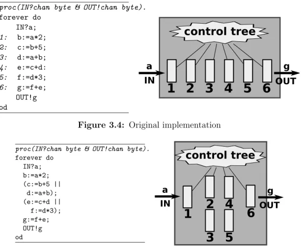
3.4 Original implementation . . . 49

3.5 Parallelized implementation . . . 49

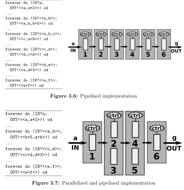
3.6 Pipelined implementation . . . 50

3.7 Parallelized and pipelined implementation . . . 50

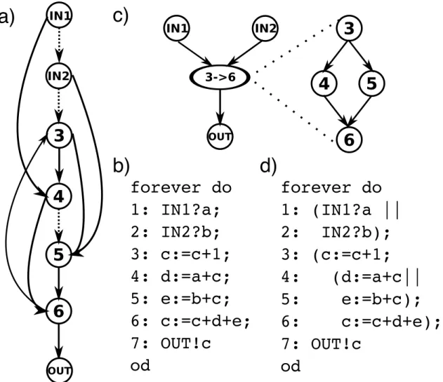
3.8 Handling cycles: a) cyclic dependency graph, b) corresponding source, c) treating cycle as atomic statement, and d) optimized source. . . 52

(16)

3.10 Operator pipelining via source code . . . 59

3.11 Replacing conditionals with conditional assignments . . . 60

3.12 Early and late decision in conditionals . . . 62

3.13 Communication optimization via directed graph . . . 65

4.1 Single-token, shared-resource design flow . . . 74

4.2 Illustration of differences between synchronous (left) and asynchronous (right) scheduling . . . 78

4.3 DFG example annotated with ST T S and ST T F properties (each oper-ation executes for 8 time units) . . . 84

4.4 Partial expansion of search space for a three-statement DAG . . . 86

4.5 Pruning via lexicographical ordering . . . 89

4.6 Basic algorithm for resource-constrained time-minimization . . . 92

4.7 Algorithm for selecting child nodes in the DAG . . . 93

4.8 Allocation search space for two function unit types . . . 98

4.9 Algorithm for area-constrained time-minimization . . . 99

4.10 Algorithm for time-constrained area-minimization . . . 101

4.11 Full expansion of the DAG for a two-operation DFG with one ALU and one multiplier . . . 105

5.1 Multi-token, shared-resource design flow . . . 118

5.2 Simple code example . . . 121

5.3 a) Unfolded and b) folded dependence graphs . . . 122

5.4 Adding a) data, b) buffering, and c) resource arcs to the graph . . . 124

5.5 Inferring buffering requirements and modeling buffer delays . . . 126

(17)

5.7 a) Buffer and b) forking data latch implementations . . . 134

5.8 Shared resource implementation . . . 136

5.9 Basic optimal area-minimization algorithm . . . 139

5.10 a) Original DFG, b) block-partitioned DFG, and c) block-partitioned DFG after blocks Y and Z are scheduled and simplified . . . 144

5.11 BlockY and its associated internal interface nodes, A, B, and C . . . . 147

5.12 Simplifying the internals for BlockY (reverse path not shown for original graph) . . . 148

5.13 Performing a single-path approximation on Block Y (reverse path not shown) . . . 150

5.14 Modeling a block interface as a canopy graph . . . 151

5.15 Removing redundant arcs from the canopy graph . . . 153

5.16 Na¨ıve approximation of throughput constraints . . . 154

5.17 Our method’s approximation of throughput constraints . . . 155

5.18 Converting a block to a two-port representation . . . 157

5.19 Conditional assignment . . . 159

5.20 Early evaluation . . . 160

5.21 a) Loop body without control elements and b) loop body with control elements inserted . . . 163

5.22 Composing sequential blocks into a single block . . . 166

5.23 Composing parallel blocks into a single block . . . 167

5.24 Basic hierarchical area-minimization algorithm . . . 169

6.1 Full expansion of the DAG for a two-operation DFG with one ALU and one multiplier . . . 183

6.2 Allocation search space for two functional unit types . . . 186

(18)

6.4 Algorithm for de_dt based energy minimization . . . 193

6.5 Parallel example of de_dt scaling . . . 193

6.6 Sequential example of de_dt scaling . . . 194

6.7 Algorithm for dE_dL based energy minimization . . . 196

6.8 Example of abutment in dE_dL scaling . . . 197

(19)

LIST OF ABBREVIATIONS

ALU Arithmetic and Logic Unit

ASIC Application-Specific Integrated Circuit

AST Abstract Syntax Tree

CDFG Control/Data-Flow Graph

DAG Directed Acyclic Graph dE

dL Derivative of total energy consumption with respect to total latency de

dt Derivative of operation energy consumption with respect to time

DFG Data-Flow Graph

DSE Design-Space Exploration

FPGA Field-Programmable Gate Array

GALS Globally-Asynchronous Locally-Synchronous

HDL Hardware Description Language

HLS High-level Synthesis

NoC Network-on-Chip

(20)

Chapter 1 Introduction

1.1 Motivation and Goals

1.1.1 Domain

Most of digital hardware today is clocked or synchronous. However, synchronous hard-ware design is facing significant challenges as we push for higher clock speeds and more complex chips. Aside from the incredible task of optimizing designs year after year, physical properties of circuits at the current scale and speed are becoming major roadblocks. For example, skew associated with high-fanout clock signals puts a great burden on the designer by increasing design time, transistor variability reduces the yield of chips at fabrication, and energy consumption at low process sizes and billions of transistors burdens the consumer (as well as the environment). Because of variabil-ity, designers must either slow chips by introducing large safety margins or contend with lower yields.

(21)

time, we must improve designer efficiency by reducing design effort. Moore’s law sug-gests that more transistors will become available, and, as a result, designer productivity must go up to produce more complex chips in the same time frame. Therefore, we need to be able to re-use components; they must be flexible and modular. Unfortunately, clocking interferes with re-usability due to global timing requirements.

Beyond conventional computing, emerging technologies are trending increasingly towards domains where global clocks become impractical. Multi-core and distributed systems, globally-asynchronous locally-synchronous systems (GALS), and network-on-chip (NoC) are examples where the top-level system integration is already becoming elastic in nature. Technologies even further out on the horizon, such as quantum and DNA-based computing are expected to have unpredictable timing as well, further highlighting the need for an alternate paradigm to global clocking.

Due to these demands, asynchronous or “clockless” design is emerging as a promis-ing alternative to synchronous design with the potential of alleviatpromis-ing many of the next generation design challenges. Rather than relying on a clock to manage the flow of computation, a request and acknowledge handshake paradigm is used to control com-putation. As a result, managing large-scale clock distribution is avoided (improving energy efficiency). Asynchronous chips are robust to changes in voltage and tempera-ture, more resistant to the side effects of process variation, and produce significantly less electromagnetic noise. Chips can also be designed with average case throughput in mind, rather than the worst case with clocking. Perhaps most important is that designs can be much more modular: rather than managing a deep clock tree, only local timing assumptions at a modules interface must typically be considered.

(22)

ASICs, the research results produced may certainly be applicable to many other do-mains, from synchronous design to multi-core computing to distributed systems.

1.1.2 Objectives

Despite the significant advantages asynchronous design can provide, several challenges remain to be addressed before greater mainstream adoption. The primary challenge of asynchronous design is that the current design tools are much less mature than syn-chronous design tools. As a result, designers who have practiced synsyn-chronous design for several decades may not easily make the switch to an asynchronous paradigm. There-fore, the majority of the research in this dissertation is aimed at making asynchronous design easier by reducing designer effort and improving performance. This dissertation focuses on building a top-to-bottom design flow to address this challenge.

The objective of this work is to produce a fully-automated design flow that:

• boosts performance through a suite of optimizations, including: parallelization, pipelining, loop-pipelining, arithmetic decomposition and decoupling (including at the bit-level), and communication optimization,

• provides design-space exploration by performing the synthesis tasks of scheduling, allocation, and binding of shared resources in an automated fashion, and

• allows a whole spectrum of designs to be explored by varying constraints, with implementations ranging from highly pipelined to control-driven, as well as ex-ploring the space in-between,

(23)

1.1.3 Thesis Statement

Design-space exploration of asynchronous systems can be automated effectively in or-der to rapidly produce high-quality implementations with significantly reduced designer effort.

1.2 Past Approaches and Current Challenges

While several approaches have been previously proposed to target high-level synthesis, none have effectively traded off optimality, performance, and other performance metrics while simultaneously allowing for rapid, easy design.

Two of the most well-known synthesis tools for the design of asynchronous systems — Haste (Haste, 2008) and Balsa (Edwards and Bardsley, 2002; Bardsley and Edwards, 2000) — rely on syntax-directed translation of behavioral specifications. Produced cir-cuits match the input specification one-to-one: every language construct in the spec-ification is directly implemented as a distinct hardware object, all sequencing in the specification is preserved, and every arithmetic operation becomes a distinct arithmetic unit (no automated resource sharing). This paradigm allows for rapid design times; however, performance of produced circuits is quite low (e.g., 10-100MHz for Haste) and span large areas on chip.

(24)

Several other synthesis approaches exist in the asynchronous domain. Budiu et al. (Budiu, 2003) introduced the approach of spatial computation, which compiles ANSI C specifications directly into hardware. However, this approach explicitly forbids re-source sharing; each computation is given its own dedicated function unit. A recent approach by Gill (Gill, 2010) targets analysis and optimization of existing pipelined systems constructed in a hierarchical fashion, but cannot handle sharing of resources.

De-synchronization (Cortadella et al., 2006; Andrikos et al., 2007) is an entirely different approach in which existing synchronous tools are leveraged to create a syn-chronous netlist, which is later converted into an asynsyn-chronous version by removing the clock and replacing it with local asynchronous controllers. While this approach leverages the significant research behind mature synchronous design tools, replacing low-level clock signals with handshaking does not allow the designer to exploit system-level concurrency as well as a top-down asynchronous design approach.

Many well-known synchronous approaches exist that specifically target performance enhancement through optimization. A recent approach by Kondratyev et al. (Kon-dratyev et al., 2011) performs synthesis that targets high performance implementa-tions; the authors’ primary aim being feasible, real-world design-space exploration. The SPARK (Gupta et al., 2003) framework converts high-level specifications in C to VHDL, performing several powerful high-level optimizations such as parallelization and loop transformation in the synthesis process. AutoPilot/AutoESL (Coussy and Morawiec, 2008) is a proprietary solution for converting specifications written in C variants to FPGAs. These tools and methods specifically target the synchronous realm and therefore are not easily transferable to the synchronous realm; as I will show later, na¨ıvely porting synchronous design methodologies to asynchronous design may result in suboptimal solutions.

(25)

asyn-chronous (Beerel et al., 2010; Taubin et al., 2007) and synasyn-chronous (Coussy and Moraw-iec, 2008) approaches are available.

Despite the breadth of research in this area, there remains a need for an asyn-chronous design flow that can produce fast, resource-shared implementations with mini-mal design effort. This thesis attempts to fill that void by contributing a comprehensive design flow, one that permits rapid design and allows the designer to easily trade-off and optimize for several performance metrics.

1.3 Contributions

In this section I will outline the contributions made in this thesis, starting with the proposed design flow, then stepping through chapter-by-chapter to highlight the contri-butions discussed in each. The contricontri-butions made in this thesis have been published in (Hansen and Singh, 2008; Hansen and Singh, 2010b; Hansen and Singh, 2010a; Hansen and Singh, 2012; Gill et al., 2006; Gill et al., 2009).

1.3.1 Proposed Design Flow

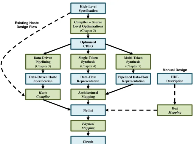
The proposed design flow is shown in Figure 1.1. In this figure, italicized items indicate existing tools. Paths with dashed arcs represent existing design flows.

(26)

My proposed design flow is shown in the center of the figure. Here, a choice of three options is presented. The leftmost path is a data-driven pipelining flow, described in Chapter 3, that performs a source-to-source conversion of a behavioral specification into an equivalent data-driven pipelined source specification. This path does not perform any automated resource sharing for conserving area, instead targeting high-performance pipelined implementations. This path leverages the existing Haste tools as a back-end. The center path provides an alternate approach that performs resource sharing in a synthesis step. This path allows the designer to trade off area, performance, power, and energy using an automated design-space exploration approach. This approach will be described primarily in Chapter 4, with energy and power considerations discussed in Chapter 6.

The rightmost path provides a hybrid approach, combining both resource-sharing and high-performance pipelining to target high-performance, low area circuits. This section will target synthesis using a multi-token scheduling approach, one in which multiple instances of a problem are being solved concurrently by the circuit. This approach is described in detail in Chapter 5.

Now, let us step one-by-one into each chapter, illustrating how the contributions made in each allow paths in the proposed designed flow to be realized.

1.3.2 Compiler and Source-Level Optimization

(27)

High-Level Specification!

Compiler + Source Level Optimizations!

(Chapter 3)!

Optimized!

CDFG!

Data-Driven Pipelining! (Chapter 3)!

Multi-Token!

Synthesis! (Chapter 5)!

Single-Token!

Synthesis! (Chapter 4)!

Data-Driven Haste Specification!

Haste! Compiler!

Data-Flow Representation!

Pipelined Data-Flow Representation!

Netlist!

Architectural Mapping!

Physical! Mapping!

Circuit!

Existing Haste Design Flow

HDL!

Description! Tech! Mapping!

Manual Design

(28)

language (Haste), to be fed into an existing syntax-directed design flow. In addition to having its own synthesis path, the proposed compiler also produces an intermediate representation that is used in the other two synthesis paths, described in Chapters 4 and 5.

1.3.3 Optimal Resource Sharing and Scheduling

In Chapter 4 I attack the problem of resource sharing in high-level synthesis. Unlike the area-hungry approach of Chapter 3 that focuses solely on performance, this chapter will present a shared-resource approach to high-level synthesis that is both fast and optimal. I will present a novel string-based formulation to the scheduling problem and an efficient branch-and-bound strategy to target the problem of resource scheduling, allocation, and binding in an optimal fashion. This chapter will introduce several tight bounds and optimizations in the branch-and-bound framework that effectively prune the scheduling and allocation search spaces, enabling the designer to explore a wide variety of potential solutions in a short period of time.

(29)

1.3.4 Pipelining With Shared Resources

Chapter 5 will present an alternate synthesis approach for shared-resource architectures, in which a high-performance, minimal-area pipelined implementation is the ultimate goal. Unlike Chapter 4, which focused on latency as a performance metric, this chap-ter will target throughput as a constraint, and as a result produce multi-token (i.e., pipelined) schedules. In this chapter I will introduce a pipelined data-flow architec-ture in which data travels directly from source to destination with optimal buffering, synchronizing only when data is needed for computation. The target architecture is distinct from the data-driven pipelines of Chapter 3.

In this chapter I will introduce a pipeline synthesis method for minimizing area under a throughput constraint, allocating the minimum number of function units and buffers required to meet the performance target. I will extend this optimal method for use with large, real-world examples via a heuristic hierarchical approach; this approach will be robust enough to handle both loops and conditionals, allowing for a rich set of input specifications. This approach provides a method for exploring a full spec-trum of designs, ranging from high-performance pipelines to low-area, control-driven implementations, simply by tightening and relaxing constraints.

1.3.5 Energy and Power Considerations

(30)

minimization, and area minimization under the bounds of energy, power, latency, and area.

In this chapter, I will also present a strategy for minimizing energy by performing voltage scaling as a post-scheduling step, in order to squeeze out even more energy savings by exploiting available slack in the schedule. This section will incorporate both heuristic and optimal methods for energy minimization, as well as a method to minimize energy while limiting the number of unique voltage levels.

1.4 Significance of Contributions

My work in Chapter 3 is thefirst approach for automatic rewriting of asynchronous high-level specifications through parallelization and pipelining to obtain higher concurrency. As a result, my approach obtains dramatic performance improvements even while using an underlying syntax-driven translation tool. This work overcomes a significant and long-standing shortcoming of state-of-the-art asynchronous design flows, which tend to be syntax-driven (Haste, 2008; Edwards and Bardsley, 2002). By efficiently transform-ing the specification through automated parallelization and automated pipelintransform-ing ustransform-ing my approach, the same syntax-driven tools can now produce implementations that are much more concurrent and, therefore, yield higher performance.

(31)

Prior to this work, the problem of optimal resource sharing for pipelined (i.e., multi-token) systems has been an unsolved problem, for both synchronous and asynchronous systems. The work in Chapter 5 is the first exact approach, whether synchronous or asynchronous, for optimal resource sharing in multi-token systems. Prior approaches have generally solved only a part of this problem, e.g., some assume the number of tokens is given, some use a discrete-time approximation, others are heuristic. My ap-proach is the first to optimize over the full joint search space consisting of all allocations, schedules and bindings of resources, all possible buffer insertions (i.e., slack matching), and all token counts. Efficient search space pruning techniques are introduced to make this approach efficient; further speed up and scalability to larger problem sizes is ob-tained by my hierarchical method.

The majority of prior approaches to resource sharing (synchronous as well as asyn-chronous) do not consider power or energy as part of the scheduling step. The ap-proaches that do consider these metrics typically treat power or energy only as sec-ondary cost functions, or only provide heuristic solutions. My approach of Chapter 6 incorporates total energy consumption and peak power dissipation as first-class cost functions during the scheduling step. To the best of my knowledge, this is the first exact approach to provide optimal resource sharing under energy/power constraints.

(32)

relative order approach is not only applicable to, but highly efficient for, synchronous systems as well. Similarly, the work of Chapter 3 is likely to be applicable to syn-chronous systems as well because at the behavioral level there is little to distinguish asynchronous and synchronous systems.

1.5 Organization of Thesis

(33)

Chapter 2 Background

In this chapter I will provide background on several important concepts that will be relevant for the remainder of the thesis. The following topics will be reviewed:

• Section 2.1 discusses asynchronous architectures, including pipelined and shared-resource implementations. I will also discuss the method of “slack-matching”, in which buffers are inserted in order to improve the performance of a circuit.

• Section 2.2 provides background on silicon compilation, from source code to cir-cuit. A discussion of source languages, graphical models for intermediate repre-sentations, and design flows is provided.

• Section 2.3 describes the analysis techniques we will use in this thesis, including canopy graphs, the cycle metric, and simulation-based methods. I will also define the terms we will use to describe the performance of a circuit, such as latency and throughput.

2.1 Asynchronous Architectures

(34)

parallelism, possibly at the cost of high area consumption. Next, I will discuss shared-resource architectures, in which shared-resources are shared to conserve area, possibly at the cost of performance. Finally, I will briefly introduce the concept ofslack-matching via buffer insertion, which is often necessary to improve performance in pipelined systems.

2.1.1 Pipelined Architectures

Pipelining is a common technique used in both synchronous and asynchronous design to improve the throughput of a design. In pipelining, computation is fragmented into multiple portions that can be performed independently; each portion is given its own dedicated hardware for storage and computation. Because each stage in the pipeline has its own dedicated set of resources, it can operate on a different instance of a problem than its neighbor, much like an assembly line.

In this way, multiple instances of a problem are computed at once, improving per-formance as a whole, although the time associated with a specific problem instance may go up due to overheads in the pipelining process. Aggressive, fine-grained pipelining can result in very high performance circuits since many problems are being solved con-currently. However, pipelining comes at a cost of area, particularly increased storage to hold the data associated with each problem instance, as well as resource area associated with each dedicated function unit.

2.1.1.1 Pipeline Stages and Styles

(35)

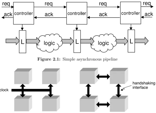
Figure 2.1: Simple asynchronous pipeline

clock

handshaking interface

Figure 2.2: Synchronous vs. asynchronous communication

right neighbor. This behavior is unlike that of a synchronous approach (Figure 2.2), in which signals are received from a global clock to latch data.

(36)

Aside from the variety in handshake protocols, data can also be encoded in multiple different ways. Bundled data (Sutherland, 1989) is a common approach in which a single wire is dedicated to each bit, and the data itself is combined with a control signal with amatched delay that corresponds to the computation time of logic between the stages. Dual-rail encoding (Williams, 1991) is a different paradigm where two wires are associated with each bit of data; some combination of signals on the two wires indicate that computation has completed. This type of encoding is more robust to timing variation, but will incur an additional area penalty due to completion detection. Several different pipeline styles exist, from GasP (Sutherland and Fairbanks, 2001) to MOUSETRAP (Singh and Nowick, 2001) to Sutherland’s micro-pipelines (Suther-land, 1989) to high-capacity (Singh and Nowick, 2007) pipelines. The work presented in this thesis targets two-phase, bundled-data pipelines, but is certainly amenable to other styles as well.

2.1.1.2 Data-flow Pipelines

In this thesis, I will refer to data-flow pipelines as pipelines in which each individual piece of data travels through the architecture without any unnecessary synchronization. That is, each stage will consist solely of data belonging to one “variable”, and will travel along a channel until it synchronizes with another piece of data only as needed to perform a computation.

(37)

2.1.1.3 Data-driven Pipelines

Data-driven pipelines are proposed in Chapter 3 as an alternative to data-flow pipelines. In these pipelines, slack-matching has been explicitly performed via construction; large blocks of data are synchronized at once and referred to as the “context” of an individual problem. As data accumulates, the size of each synchronized buffer increases; as data is consumed and is no longer needed in the pipeline, it is dropped from future synchronized buffers. This type of pipeline consists of large, linear blocks with minimal fork and join constructs, in contrast to data-flow pipelines that have lightweight buffers and complex topologies.

While data-flow pipelines are more efficient; data-driven pipelines are found in ex-amples such as common pipelined processors, which may have several stages (i.e., fetch, decode, execute). Data is not directly passed from source to destination, but typically goes through every stage even if a stage does not operate on the data.

2.1.2 Shared-Resource Architectures

Shared-resource architectures are an alternative to asynchronous pipelines. Unlike pipelines, in which control is distributed, shared-resource architectures generally rely on a global controller to transfer data between function units and registers. An example of such an architecture is illustrated in Figure 2.3.

In this figure, a large, monolithic control block is connected to a set of multiplexers that control the flow of data into function units. This control block is also connected to a set of registers to determine which register will latch the result of computation. Here, the complete schedule of data transfer is encoded in the controller, unlike in pipelines where data itself triggers computation.

(38)

Control FSM

MU

X Function _Unit

R

EG

R

EG

MU

X Function _Unit

R

EG

MU

X

MU

X

MU

X

Figure 2.3: Shared-resource architecture

other flavors may exist, the most common element of a shared-resource architecture is control-directed transfer of data between shared registers and resources.

2.1.3 Buffering Requirements (Slack-Matching)

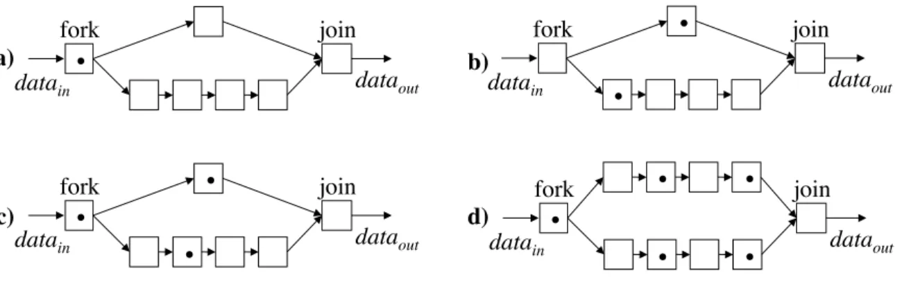
Slack-matching is a technique used by designers to reconcile two paths that have mis-matched latencies or storage capacities. A slack-mismatch is a performance concern that results in reduced throughput, as data cannot enter a pair of forked pipelines if one of the paths is already full. By adding additional buffers on one of the paths, a slack-mismatch can be alleviated, and performance improved.

(39)

data_in_! data_out_!

fork_! join!

a)! _•_!

fork_! join!

b)!

•!

fork_! join!

c)!

•! •!

•! datain! dataout!

fork_! join!

d)! _•_!

•!

Figure 2.4: Slack mismatch example

due to a lack of buffer space in the shorter path.

Consider the operation of this pipeline. To begin, a piece of data enters the start of the pipeline on the left (Figure 2.4a). The data then splits and travels down each path, to be synchronized at the join node later in the pipeline (Figure 2.4b). A new piece of data can then enter, ready to start computation on both forks (Figure 2.4c). However, the data is stalled because there is no space for it on the shorter path.

By inserting additional buffers on the shorter path, additional room is available on the shorter path, allowing data to enter, thus alleviating the slack-mismatch (Fig-ure 2.4d).

The problem of slack-mismatch is automatically avoided in the approach in Chap-ter 3 by using a data-driven pipeline style. However, in ChapChap-ter 5, I incorporate the slack-matching problem into the proposed synthesis method in order to slack-match the data-flow pipelines that are generated by that method.

2.2 Languages, Representations, and Compilation

(40)

such as abstract syntax trees, data-flow graphs, and Petri nets. Finally, I will give an overview of existing asynchronous design flows, such as the syntax-directed Haste and Balsa design tools, as well as review more general synthesis approaches, including those that attack the common constrained-optimization problem for scheduling, allocation, and binding of shared resources.

2.2.1 Behavioral Description Languages

2.2.1.1 Overview

The breadth of potential languages for performing asynchronous high-level synthesis is wide; some designers use software programming languages such as C for their high-level descriptions, while others use common hardware languages such as Verilog and VHDL, and yet others utilize highly-specialized languages for asynchronous design, such as Haste and Balsa. There are several factors that weigh into the selection of a language; two common desires are tool support and richness of the specification language.

Two syntactical features designers often require in a hardware description language are channel communication to transmit data between modules, and a simple, explicit means for representing parallelism in the specification. Unfortunately, these features are often lacking in software programming languages, hence specialized hardware languages are often a better match.

(41)

& byte = type [0..255]

& byteplus = type [-255..255]

& GCD: main proc(IN?chan <<byte,byte>> & OUT!chan byte). begin

& ab: var <<byte, byte>> ff & a=alias ab.0

& b=alias ab.1

& s: var byteplus ff | forever

do IN?ab;

do a # 0 then s := a-b;

<<a,b>> := if sign(s) then <<b,a>> else <<s,b>> fi

od; OUT!b od end

Figure 2.5: GCD example

2.2.1.2 Haste Language

Let us focus on the primary source language used by our approach: the Haste language. Some key Haste constructs are as follows:

• channel reads (IN?ab ) • channel writes (OUT!b ) • assignments ( s:=a-b ) • tuples (<<a,b>> )

• sequential composition ( b:=a+x ; c:=b+y ) • parallel composition ( a:=b+x || c:=d+y ) • loop control ( forever do ...od )

(42)

• procedure definition ( GCD: main proc(...). )

• conditional assignment ( x:= if bool then y else z fi )

Figure 2.5 shows the Haste specification of a very simple program that computes the GCD of two numbers. The program has one input channel, IN, through which it receives two data items from the environment in a tuple (pair of bytes). It also contains an output channel OUT, through which it transmits results to the environment. Each channel consists of a pair of request-acknowledge wires along with the data wires.

In the specification, ab and s are all storage variables, while a and b are merely aliases/pointers to variables in the tuple ab. The main construct in the body of the specification is a forever do loop. This loop reads from the input channel, then enters a second loop that computes the GCD of the input numbers. Once the GCD is computed, it transmitted to the environment on the output channel,OUT.

The conversion of these language constructs into a final hardware representation will be discussed in Section 2.2.3.3.

2.2.2 Graphical Representations

The first step in the compilation process is to transform the human-readable behav-ioral specification into a form that is amenable to processing and optimization by the compiler. Generally, this new form is an intermediate representation that often takes a tree-like or hierarchical structure,e.g., an abstract syntax tree. Now, let us consider several common graphical representations that are used either by the compiler, or by the designer, in order to represent a specification or model its performance.

2.2.2.1 Abstract Syntax Tree

(43)

while (a!=0){

!

a=a-1;

!

c=d*e;

!

}

!

while

!

!=

!

a

!

0 !

;

!

=

!

a

!

-

!

a

!

1 !

=

!

c

!

*

!

d

!

e

!

cond body

loc exp loc exp

Figure 2.6: Abstract syntax tree example

a one-to-one fashion with source code constructs. Figure 2.6 illustrates a sample AST for a while loop. Here each construct is converted directly into a node; the while loop becomes a control construct with two children, a conditional and a loop body. The conditional is a binary not-equal operation that requires two children, in this case the variable a and the literal 0. The remainder of the graph is constructed in a similar fashion.

After the AST has been generated, the compiler performs several annotations, such as those linking a variable name to its declaration and type, determining bit-widths for operations, and so on. A compiler may perform optimizations here as well, such as conversion to single-static assignment form, dead-code removal, etc.

2.2.2.2 Control Data-Flow Graph

(44)

a=x+y;

!

b=a*y;

!

c=a-b;

!

d=b*b

!

y

!

a

!

x

!

b

!

c

!

d

!

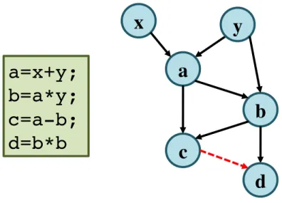
Figure 2.7: Control/data-flow graph example

operations, and arcs between these nodes that represent the flow of data.

A data-flow graph can be extended to incorporate control information, such as loops and conditionals. This extension is called a control/data-flow graph (CDFG). In Chapter 5, a similar construct is used, a folded-dependence graph. This type of graph incorporates data dependencies between operations, and then inserts additional control elements, including scheduling arcs, control constructs such as loops and conditionals, and write-after-read dependencies from which buffering is inferred.

A sample CDFG is shown in Figure 2.7. In this example, the dependence between

cand d is purely control, rather than data, and is shown as a dashed red arc.

2.2.2.3 Petri Nets

A Petri net is a mathematical representation that is often used for modeling concurrency in systems. Petri nets have a wide range of uses; they can be used for simulation of operation, to determine correctness of an implementation, to test for deadlocks, etc. A formal definition of Petri nets is not required for this thesis; however, a basic introduction can provide some insight.

(45)

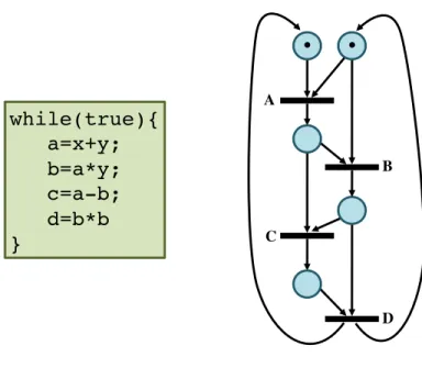
while(true){! a=x+y;! b=a*y;! c=a-b;! d=b*b! }!

A!

B!

C!

D!

•

Figure 2.8: Petri net example

to model data or control transfer. A place is a storage location for tokens, an arc is a path on which a token can travel, and a transition is a guard that synchronizes data or control. A sample Petri net is shown in Figure 2.8.

The behavior of a Petri net is as follows. First, tokens are placed in the graph in an initial marking, which enables some set of transitions (otherwise the Petri net is not live). However, a specific transition cannot fire until all of its incoming arcs have a token available, at which point the transition becomes enabled. When a transition fires, a token is consumed from each input arc to the transition, and a token is produced on each output arc from the transition, to arrive at a new place. A new marking is produced, and the Petri net can continue operation by firing another transition.

(46)

HDL! Specification!

Compiler! Front-end!

Intermediate! Representation!

Synthesis!

Netlist!

Physical! Mapping!

Circuit!

Figure 2.9: Common high-level synthesis flow

nets were used as an initial model in Chapter 4, while marked graphs were used as an initial model in Chapter 5.

2.2.3 Compiler Flow

Now that I have discussed languages and representations used in the compilation pro-cess, let me now describe the flow of compilation in high-level synthesis (HLS).

(47)

optimizations and synthesis tasks such as scheduling, allocation, and binding of shared resources. Finally, this modified representation is sent to a back-end for conversion to hardware.

2.2.3.1 Source to Intermediate Representation

The first step in the hardware compilation process is to convert the input specification into an intermediate representation; this is often described as the front-end of the compiler. As with software compilers, an HLS compiler will step through the common steps of lexical, syntactic, and semantic analysis in order to convert the source to an intermediate representation. The compiler implemented in Chapter 3 is a recursive-descent compiler that converts a Haste specification into an annotated AST. After the intermediate representation is produced, optimizations may be performed prior to being output by the back-end of the compiler.

2.2.3.2 Synthesis

Once an intermediate representation is created, the next step is to convert it to hard-ware. In this thesis I will consider two main forms of synthesis. The classic synthesis problem is one of performing resource sharing as part of a constrained-optimization problem. Chapters 4 and 5 will focus on this type of synthesis. An alternate method is syntax-directed translation, which is used by the Haste compiler

Let us describe first three main steps of synthesis:

(48)

• Scheduling is the step where the designer or design tool determines the order of execution for a set of operations that share the same type of resources. The goal of scheduling is often to optimize a performance metric, such as maximizing throughput or minimizing latency. Alternatively, scheduling may target low-energy or low-power by scheduling execution appropriately, such as by scheduling operations on less power-hungry function units, or spreading execution out across the time domain.

• Binding is the step where schedules and operations are mapped onto specific pieces of hardware,i.e., resource instances. As an example, an operation may be scheduled to execute on a type of function unit at a specific time, but the specific function unit instance may not yet have been determined. The binding step will finalize these mappings; this is important because different bindings may lead to different multiplexing costs (in terms of both area and delay).

Often a designer will use a synthesis approach to explore a full design space in order to balance or optimize for specific metrics, such as area, performance, energy, etc, as in Chapters 4 and 5. An alternate route is to generate a final implementation via construction; i.e., applying a specific set of transforms and mappings to create an implementation without exploring a full design space. In Chapter 3, the proposed compiler creates a data-driven implementation by applying a series of transforms that can be manually enabled or disabled by the designer, then the syntax-directed Haste compiler converts the optimized specification in a one-to-one fashion into hardware.

2.2.3.3 Syntax-Directed Translation

(49)

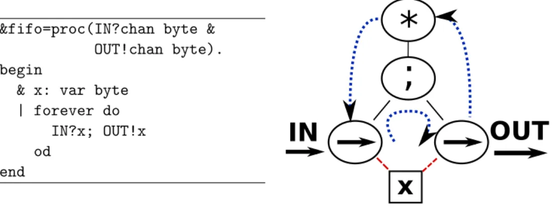
&fifo=proc(IN?chan byte & OUT!chan byte). begin

& x: var byte | forever do

IN?x; OUT!x od

end

Figure 2.10: Haste example

with the source specification; each language construct typically translates to a specific hardware library component. This paradigm makes the process very transparent to the designer, but without manual optimization, syntax-directed translation may lead to lower performance. Two of the more mature syntax-directed translation approaches to synthesis are the Haste and Balsa design flows.

2.2.4 The Haste Design Flow

(50)

In summary, the compilation approach is quite simple but very powerful: fairly complex algorithms can be easily mapped to hardware. Gate-level implementations for complex designs, such as complete micro-controller, can be generated from a few hundred lines of high-level code.

In this work, I will use the syntax-directed paradigm in Chapter 3, but only after per-forming various automated optimizations (code rewritings) to improve performance.

2.3 Analysis Methods

In this section I will describe several common analysis methods for determining the performance of asynchronous pipelines. I will start by giving definitions of latency, throughput, and cycle time: key metrics used in this thesis. Next, I will describe canopy graphs, a useful tool for determining the throughput bound of a pipelined system. Then, I will discuss the cycle metric mean problem and its performance implications. Finally, I will discuss how simulation can be used as a tool for analyzing performance.

2.3.1 Performance Metrics

There are three key performance attributes we will be concerned with in this thesis: latency, cycle time, and throughput.

2.3.1.1 Latency

(51)

chapters.

For a schedule, latency will refer to the time it takes for a complete execution of every operation in a specification, from start to finish. In essence, this refers to the time from when the first action begins in the schedule to when the final action completes.

In the context of pipelining, the latency of a pipeline is similar; here, the forward latency of a pipeline is the time it takes for a token to travel from the start to the end of an empty pipeline (i.e., from input to output). Similarly, the forward latency of a pipeline stage is the amount of time it takes for data to propagate from that stage to the next. IfFi represents the forward latency of a stageiin a pipeline, then the overall forward latency of a linear pipeline is:

F =X

∀i

Fi

Correspondingly, the reverse latency of a pipeline is the time it takes for a “hole” to propagate from the end of the pipeline to the start of the pipeline (e.g., from output to input) if the pipeline is initially filled. Thus, the reverse latency is determined by the speed at which acknowledgments propagate backwards. If the reverse latency of a stage i in a pipeline isRi, then the reverse latency of a linear pipeline is:

R =X

∀i

Ri

Often the designer will be tasked with minimizing the latency of a schedule or partial schedule in order to meet a set of constraints.

2.3.1.2 Cycle Time

(52)

As an example, in a linear pipeline, the cycle time can refer to the amount of time that elapses between outputs produced by its final stage, or, similarly, the amount of time between consumption of inputs by its first stage.

The cycle time of a linear pipeline is actually tied to the cycle time of its slowest stage. In a homogeneous pipeline, in which all forward and reverse latencies are the same for each stage, the cycle time of a stage is typically equal to:

CTi =Fi+Ri

In the context of scheduling, the cycle time of a schedule is the time that elapses between two problem instances starting (or finishing) their schedules. As an example, a multi-token schedule may allow new problem instances at times 0, 20, 40. . . , and each problem instance may complete at times 100, 120, 140. . . , thus the schedule has a cycle time of 20 and a latency of 100.

2.3.1.3 Throughput

The term “throughput” refers to the inverse of cycle time. We often use throughput as an indicator of the performance of an implementation; the higher the throughput, the better the performance.

2.3.2 Canopy Graphs

Using canopy graphs for performance analysis was originally explored in the context of asynchronous pipelined rings (Williams, 1991; Williams et al., 1987). Since then, the work has been expand to linear and hierarchical pipelines (Lines, 1998), (Singh et al., 2002), and (Gill, 2010).

(53)

Occupancy!

n

!

0 !

Limiting!

Stage!

T

hroughput

!

n+1

!

n-1

!

1 !

Theoretical

!

Maximum

!

Figure 2.11: Basic canopy graph

pipeline. If the occupancy is too low, the pipeline is underutilized, and therefore it cannot achieve its maximum throughput. This is referred to as “data-limited” behavior. If the occupancy is too high, there is essentially contention for storage space; an item cannot move ahead to the next stage until that stage is vacated. In order to free up space, holes must travel backwards in the pipeline. We will refer to throughput degradation due to congestion as “hole-limited” behavior.

(54)

while the hole-limited line intersects the x-axis where the maximum occupancy of the pipeline is exceeded.

The graph is further limited by the throughput of the slowest stage; this stage’s throughput introduces the bounding horizontal line at the top. This is what leads to the “canopy”-like structure of the graph. The operating region of the graph is the full region under this set of lines.

Several extensions and generalizations to the theory of canopy graphs have been introduced, including handling parallel and sequentially composed pipelines (Lines, 1998; Gill, 2010), as well as conditional operation and loops (Gill, 2010). A full review of this work is available in (Gill, 2010), but two key observations are that the joint canopy graph of a set of parallel pipelines will be the intersection of their individual pipelines, while the joint canopy graph of sequential pipelines will be their horizontal sum.

2.3.3 Maximum cycle mean

The cycle mean is an important property of a graph that can be used to help determine the performance of an implementation. In Chapter 5, I will use a graph-based model that is amenable to the classic maximum cycle mean problem (Dasdan and Gupta, 1997), which can be employed in order to bound the cycle time of a potential solution. The computation of the cycle metric is rather simple. We begin with a cycle in a graph that has each of its arcs annotated with two values: a weight and a cost. In the scenario in Chapter 5, that cost will be a delay.

The cycle metric for cyclec in graph G is defined as follows:

Mean(c) =

P

e∈cdelay(e)

P

(55)

where e is an edge in the cycle c. The cycle mean for one cycle bounds its minimum cycle time; the specific cycle cannot work any faster. Since a typical graph may consist of many cycles (thousands or more), in order to determine the cycle time of the full graph, we must find the maximum of the cycle means for all cycles in the graph:

Cycle Time(G) = max

c∈G (Mean(c))

This metric will be utilized heavily to determine performance in Chapter 5.

2.3.4 Simulation

Simulation provides an alternate means to measure the performance of an implementa-tion. While analysis methods such as canopy graphs and the cycle metric can provide a model for performance under a certain set of conditions (i.e., steady-state behav-ior), the stochastic nature of constructs such as conditionals and loops can make such analysis imperfect at best.

For verification of the work presented in Chapter 3, the built-in Haste simulator was used. As the Haste tools have since become unavailable, I created my own discrete-event simulator to verify the performance of the work presented in Chapter 5.

2.4 Summary

(56)

(57)

Chapter 3 Data-Driven Design: Unlimited

Resources

A fundamental desire in the process of design, whether in the realm of hardware, software, or even beyond computing, is to be able to explore a complete design space to find the best possible solution. Every designer must make some trade-offs; within the design space of our problem, several unique options exist, some implementations may focus on performance, while others may focus on area, energy, or power, or any combination in-between. One key problem, however, is that exploring every possible design manually is often infeasible within a reasonable time frame.

(58)

High-Level Specification!

Compiler + Source Level Optimizations!

(Chapter 3)!

Optimized!

CDFG!

Data-Driven Pipelining!

(Chapter 3)!

Multi-Token!

Synthesis!

(Chapter 5)!

Single-Token!

Synthesis!

(Chapter 4)!

Data-Driven Haste Specification! Haste! Compiler! Data-Flow Representation! Pipelined Data-Flow Representation! Netlist! Architectural Mapping! Physical! Mapping! Circuit! Existing Haste Design Flow HDL! Description! Tech! Mapping! Manual Design

Figure 3.1: Data-driven design flow

for shared resources.

(59)

3.1 Introduction

Because of the syntax-directed nature of existing asynchronous design tools, generating high-speed implementations can be an arduous process. The best-known tools (e.g., Haste/Tangram (Haste, 2008), and Balsa (Bardsley and Edwards, 2000)) use syntax-directed translation to compile behavioral specifications directly to circuits, with few high-level optimizations. In this type of design flow, each language construct directly maps to a specific hardware component. Therefore, the performance of a specification depends on the amount of optimization the designer manually performs. Straight-forward specifications often have low performance due to unnecessary sequencing and unpipelined operation. As a result, designers must either contend with relatively slow implementations or bear the burden of writing highly optimized specifications them-selves.

Burdening the designer with optimizing a specification has several drawbacks. First, writing highly concurrent code entails much effort and is error-prone. Second, such code often lacks readability and maintainability, and is therefore hard to modify and reuse. Finally, such a manual approach hinders automatic design-space exploration. In an ideal design flow, performance analysis tools are typically used to identify bottlenecks in the system, and then local modifications are applied to remove the bottleneck; this procedure is repeated until desired performance is achieved. Therefore, code rewriting should ideally be automated.

This chapter introduces an alternative to manual optimization: an automated “source-to-source” compiler that transforms one behavioral specification into another behavioral specification with significantly higher concurrency. The proposed approach introduces a suite of transformations:

(60)

• pipelining for increasing concurrency within a statement group,

• arithmetic optimization for increasing concurrency at the sub-statement level, and

• re-ordering of channel communicationfor increasing concurrency across modules.

As a result, designers can write straightforward behavioral code, focusing mainly on its functional correctness rather than on concurrency and performance. The code is automatically transformed by the proposed source-to-source compiler to be highly con-current, and then passed back through the original Haste design flow.

The two techniques of arithmetic optimization and communication reordering are core contributions of our approach. While basic parallelization and pipelining may help optimize a specification at the granularity of individual statements, there are of-ten performance bottlenecks due to individual statements with long-laof-tency arithmetic operations (e.g., 64-bit adds or multiplications). Further, a single statement may have a complex expression involving multiple arithmetic operators. The proposed approach pushes concurrency enhancement down to a sub-statement level by introducing all of the following: expression re-factoring to introduce parallelism, expression pipelining, and pipelining of individual (‘atomic’) operators. As a result, bottlenecks due to com-plex arithmetic are alleviated.

(61)

sys-tem. A conservative approach is to always maintain the original order of channel ac-tions; although safe, such an approach is suboptimal. The proposed strategy, instead, is to pursue a more optimal approach that includes a careful analysis to determine the space of legal code transformations. As a result, our approach provides greater opportunity for concurrency enhancement.

Previous approaches for improving the throughput of implementations produced by the Haste and Balsa tools have mostly focused at the circuit and intermediate (hand-shake) levels, including more optimized circuit-level designs of handshake components (e.g., more concurrent sequencers (Plana et al., 2005)), and peephole optimization and re-synthesis at the intermediate level (Chelcea and Nowick, 2002). While some of these approaches have yielded significant speedup (1.54–2.06x), they are unable to take ad-vantage of the significantly greater optimization opportunities at a higher level. As Section 3.5 shows, optimizing at the source level can provide an order of magnitude greater speedup. Moreover, the intermediate and circuit-level approaches are orthog-onal to the proposed approach, therefore they are not excluded from being applied within the design flow.

The domain of specifications targeted by the proposed approach areslack elastic sys-tems (Manohar and Martin, 1998a). A slack elastic system preserves correct operation even if extra pipeline buffer stages (i.e., extra slack) are introduced on any communi-cation channel. It was shown that a system is slack elastic if it is deadlock-free and it satisfies certain properties regarding channel probing and non-determinism (Manohar and Martin, 1998a). Since the approach introduces pipelining into a specification, the assumption of slack elasticity is a requirement.

(62)

Solu-tions (Haste, 2008), and synthesized to gate-level netlists and simulated. Experimental results demonstrate that the original specifications are correctly and efficiently rewrit-ten into highly concurrent ones. If code length is used as an indicator of designer effort, the proposed approach reduces the required effort by a factor of 3.3x on average (up to 8.8x). Alternatively, the impact can be quantified by the throughput improvement achieved by optimizing the original specification: up to 59x speedup using the basic approach, and a further 5.2x using arithmetic pipelining.

The remainder of this chapter is organized as follows. Section 3.2 reviews the Haste flow and asynchronous pipelining, then discusses related previous work. Then, Section 3.3 presents the basic concurrency-enhancing transformations. Section 3.4 discusses advanced topics, including arithmetic optimization, handling of conditionals and loops, and reordering of channel communication actions. Section 3.5 presents results, and finally Section 3.6 gives conclusions and future work.

3.2 Background and Previous Work

This section first briefly reviews the relevant portions of the Haste design flow then discusses its limitations. Next, asynchronous pipelines are briefly reviewed, along with a discussion of the distinctions between control-driven, data-driven, and data-flow design paradigms. Finally, prior related work is presented.

3.2.1 The Haste Design Flow

(63)

&fifo=proc(IN?chan byte & OUT!chan byte). begin

& x: var byte | forever do

IN?x; OUT!x od

end

Figure 3.2: Haste example

language is a close variant of the CSP behavioral modeling language (Hoare, 1985). The main Haste language constructs that are used in the presentation of this chapter are:

• channel reads (IN?x ) • channel writes (OUT!x+y ) • assignments ( a:=b+c )

• sequential composition ( b:=a+x ; c:=b+y ) • parallel composition ( a:=b+x || c:=d+y )

Figure 3.2 shows the Haste specification of a simple program, a single stage FIFO. The program has an input channel IN, through which it receives data items from the environment, and an output channel OUT, through which it transmits results to the environment. Each channel consists of a pair of request-acknowledge wires along with the data wires. In the specification, x is a storage variable. The main construct in the body of the specification is aforever do loop that performs the following actions repeatedly: (i) read a value from channel IN and store it into variablex; then (ii) write the value stored in x to the output channel OUT.

Performance Limitations. As you may recall from Chapter 2, given a

(64)

forever do IN?a; b:=f1(a); c:=f2(b); d:=f3(c); OUT!f4(d) od

Figure 3.3: Control dominated (top) vs. data-driven (bottom)

as the number of statements increase in the code snippet in Figure 3.2, the size of the control cycle increases, resulting in a higher latency block. Several handshakes in the control tree may be required before an action can occur. As a result, the performance of the system suffers. We can describe this situation as “control-dominated.”

A behavioral design flow for synthesis and optimization of asynchronous systems