Spectropolarimetry for planetary exploration

(1)

Cover Page

The handle

http://hdl.handle.net/1887/29978

holds various files of this Leiden University

dissertation

Author: Harten, Gerard van

(2)

(3)

(4)

(5)

ISBN 978-94-6259-458-6

Cover image: Spectropolarimetric measurements of

visible light with an increasing degree of linear

polar-ization from unpolarized (left) to fully polarized (right),

obtained with the Spectropolarimeter for Planetary

(6)

planetary exploration

Proefschrift

ter verkrijging van

de graad van Doctor aan de Universiteit Leiden,

op gezag van Rector Magnificus prof. mr. C. J. J. M. Stolker,

volgens besluit van het College voor Promoties

te verdedigen op maandag 8 december 2014

klokke 13:45 uur

door

Gerrit van Harten

(7)

Prof. dr. Christoph U. Keller

Co-promotor:

Dr. ir. Frans Snik

Overige leden promotiecommissie:

Dr. Matthew A. Kenworthy

Prof. dr. Jérôme C. Riedi (Laboratoire d’Optique Atmosphérique, France)

Prof. dr. Huub J. A. Röttgering

(8)

1 Introduction 1

1.1 Polarimetry of planetary atmospheres . . . 1

1.2 Earth atmosphere . . . 3

1.3 Aerosol measurements . . . 6

1.4 Light scattering and polarization . . . 7

1.5 Atmospheric scattering measurements . . . 12

1.6 Measuring polarization . . . 15

1.7 Polarimeter performance and calibration . . . 19

1.8 Brief history of SPEX . . . 20

1.9 Thesis outline . . . 21

1.10 Outlook . . . 23

2 Prototyping for the Spectropolarimeter for Planetary EXploration (SPEX): calibration and sky measurements 27 2.1 Introduction . . . 29

2.2 SPEX instrument principle . . . 30

2.3 Prototype design . . . 33

2.4 Prototype results . . . 36

2.5 Outlook . . . 41

3 Performance of spectrally modulated polarimetry I: Error analysis and optimization 45 3.1 Introduction . . . 46

3.2 Instrument . . . 47

3.3 Measurement formalism . . . 49

3.4 Error analysis . . . 53

3.5 Static errors . . . 56

3.6 Dynamic errors . . . 60

3.7 End-to-end simulation . . . 68

3.8 Conclusions . . . 71

4 Performance of spectrally modulated polarimetry

(9)

II: Data reduction and absolute polarization calibration of a prototype SPEX

satellite instrument 73

4.1 Introduction . . . 74

4.2 SPEX instrument . . . 74

4.3 Data reduction pipeline . . . 78

4.4 Polarization calibration stimulus . . . 84

4.5 SPEX polarimetric calibration . . . 89

4.6 Discussion . . . 93

5 Atmospheric aerosol characterization with a ground-based SPEX spec-tropolarimetric instrument 97 5.1 Introduction . . . 98

5.2 Measurements . . . 99

5.3 Aerosol retrieval . . . 107

5.4 Results . . . 108

5.5 Discussion . . . 110

5.6 Conclusions and Outlook . . . 112

6 Spectral line polarimetry with a channeled polarimeter 115 6.1 Introduction . . . 116

6.2 Method . . . 118

6.3 Error analysis . . . 122

6.4 Application of line polarimetry to the O2A absorption band . . . 125

Bibliography 131

Samenvatting 141

Curriculum Vitae 147

(10)

Chapter

1

Introduction

Remote characterization of atmospheric aerosols is important because of their impact

on public health and climate. To retrieve aerosol concentration and microphysical

properties, such as size, shape, and chemical composition, accurate measurements of the intensity, color and polarization of the sky are required at different scattering angles. Polarization is an intrinsic property of light, but unlike intensity and color, it is not visible to the naked eye. However, it can be made visible by filtering light with a certain polarization state using a polarizer. This is used in Polaroid sunglasses to suppress bright, strongly polarized reflections off the road or water, or in modern 3D theater glasses to create depth perception using two slightly shifted images with

different polarization states. Any interaction of light with a material, e.g. reflection,

refraction or diffraction, changes its polarization state. In fact, the polarization state of sunlight scattered by aerosols in the atmosphere carries more information about the scattering particles than the intensity.

An early example of the power of multi-angle multi-wavelength intensity and

polarization measurements is the detailed characterization of clouds on Venus from

the Earth. Instrumentation for in-orbit characterization of aerosols in the Earth’s

atmosphere is still under development; in particular the accuracy of the polarization

measurement needs an order of magnitude improvement, which requires

ground-breaking concepts for both the instrument and calibration. This drives the

develop-ment, verification, and field-deployment of the highly accurate Spectropolarimeter for Planetary EXploration (SPEX), as described in this thesis.

1.1 Polarimetry of planetary atmospheres

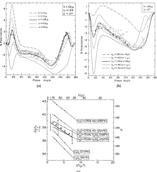
Detailed characterization of the composition of planetary atmospheres using

po-larimetry goes back to the year 1929, with Lyot’s PhD thesis presenting his "Research

(11)

on the polarization of light from planets and from some terrestrial substances" (Lyot

1929). His work includes accurate measurements of the broadband visible

polar-ization of Venus at phase angles1 of 2–176

◦

, as shown in Fig. 1.1a. The strong

polarization peak around 15

◦

indicates a rainbow, caused by liquid droplets, and

the peak around 160

◦

is typical forward scattering polarization. Comparison with

lab scattering measurements of a large variety of samples led to the conclusion that

Venus is covered in opaque clouds with droplet sizes of ∼ 2 µm and a refractive

index close to water.

In the next decades, several radiometric and spectroscopic observations

con-firmed that the Venusian surface is hidden behind opaque clouds, but their chemical

composition remained unknown. More than a dozen postulated compositions were

compatible with the observed intensity distribution across the disk, the intensity as

a function of planetary phase angle, and spectral absorption lines and bands. In

the sixties, additional polarization measurements were taken in multiple wavelength bands within 340–1050 nm by Dollfus (1966), Coffeen & Gehrels (1969), Dollfus &

Coffeen (1970). Researchers in Leiden realized the potential wealth of information

in Lyot’s and this multi-dimensional data, and developed a full radiative transfer

model, including polarization and multiple scattering (Hansen 1971, Hovenier 1971). They ran the atmospheric model for years to obtain a definitive fit for the particle size distribution (Fig. 1.1a) and the spectral refractive index (Fig. 1.1b) that showed that Venus is covered in clouds of concentrated sulfuric acid (Fig. 1.1c) (Hansen & Hovenier 1974).

These results were confirmed by in-situ nephelometer and particle size

spec-trometer measurements onboard entry probes of the Pioneer Venus Multiprobe and Venera spacecraft a few years later (Knollenberg & Hunten 1980, Marov et al. 1980,

Ragent & Blamont 1980). Compared to the disk-integrated Earth-based

observa-tions, the descents to the surface provided a detailed profile of the 60 km thick

multilayered sulfuric acid cloud and haze system, on top of the96.5%carbon dioxide

atmosphere in the lower 30 km, giving rise to a surface temperature of 740 K and pressure of 93 bar (Basilevsky & Head 2003). These extreme atmospheric conditions, obviously not compatible with human life, are believed to be the result of a runaway greenhouse effect (Rasool & de Bergh 1970).

The groundbreaking interpretation of the polarization of Venus is now applied to the modeling of polarized signals from exoplanets, and the polarimetric

characteriza-tion of aerosols and clouds in the Earth’s atmosphere. For example, disk-integrated

polarization measurements of the Earth, as if it were an exoplanet, contain informa-tion about the fracinforma-tional coverage by clouds, oceans, and vegetainforma-tion (Sterzik et al.

2012). A polarization peak is observed at the Oxygen A absorption band, indicating

a large abundance of molecular oxygen, which may serve as a biosignature. The po-larized rainbow feature provides a sensitive method for the detection of liquid water clouds on exoplanets, which is a prerequisite for life as we know it (Karalidi et al. 2012).

1

(12)

(a) (b)

(c)

Figure 1.1:The composition of the clouds that cover Venus is discovered using ground-based

polarimetry. (a)-(b) Model calculations (lines) are fitted to measurements (symbols) of the

degree of linear polarization at multiple phase angles, for various (a) particle sizesa[µm] and

(b) refractive indicesnr. (c) The chemical composition is uniquely determined as concentrated

sulfuric acid via the spectral refractive index. Figures from Hansen & Hovenier (1974).

1.2 Earth atmosphere

The scientific goal of this thesis is the characterization of the Earth’s atmosphere,

(13)

thickness of the atmosphere is only 100 km. Eighty percent of the atmosphere is

contained in the troposphere, the lowest 12 km where weather takes place. The

aerosols are mainly located in the lowest kilometer, the planetary boundary layer, where vertical mixing is strongest due to the friction of the Earth’s surface on wind, and further upward mixing is inhibited by an inversion layer. However, Saharan dust, volcanic ash, and forest fire smoke sometimes reach higher parts of the atmosphere. Heat is transported from the Earth’s surface into the troposphere via convection, so

overall the temperature decreases with altitude. In the stratosphere at 12–50 km

the temperature goes up again, due to the absorption of solar ultraviolet radiation

in the ozone layer. Less than 0.1% of the atmosphere is in the even higher layers,

where meteors burn up and aurorae take place.

1.2.1 Aerosols

Aerosols, also known as particulate matter, are particles or droplets suspended in

the air. Some types are naturally occurring, such as sea salt, desert dust, and

volcanic ash, others are mostly anthropogenic, such as sulfates, nitrates, soot, smoke

and ashes from combustion or forest fires, or ammonia salts from agriculture. The

sulfates, nitrates and ammonia salts are secondary aerosols, meaning that they

are emitted into the atmosphere as gas where they are transformed into particles,

in contrast to primary aerosols that started as particles. Aerosols typically have

lifetimes of days to weeks before they leave the atmosphere, mainly by rainout,

washout, and sweep out. A particle is rained out when a water droplet condenses

on it to the point that it precipitates in the form of a raindrop, washout occurs when a particle is incorporated in an existing droplet, and sweep out means that a particle

is bombarded by a raindrop. Because of the short lifetimes, transportation by the

wind is typically limited to 100–1000 km. The locality of aerosol sources, and their

limited transportation ranges cause large regional variations in aerosol load. Note

that the deposition of aerosols that reach stratospheric altitudes is less efficient.

For example, the eruption of Mount Pinatubo in 1991 released∼20million tons of

sulfur dioxide in the atmosphere, that transformed into a global haze of sulfuric acid,

causing a global temperature decrease of 0.5◦C for about two years (Hansen et al.

1993).

1.2.2 Climate

Aerosols and clouds influence the Earth’s climate by altering its radiative balance. Their direct radiative effect consists of the scattering of sunlight, partly back into space, as well as absorption, particularly in the case of black carbon (McCormick

& Ludwig 1967, Ramanathan & Carmichael 2008). Aerosols also affect climate

in-directly, because they can act as cloud condensation nuclei, leading to more and

smaller cloud droplets (Twomey 1977, Kaufman et al. 2005). This results in

in-creased cloud albedo (reflectivity) and longer cloud lifetimes, because the smaller

(14)

Introduction 5

12

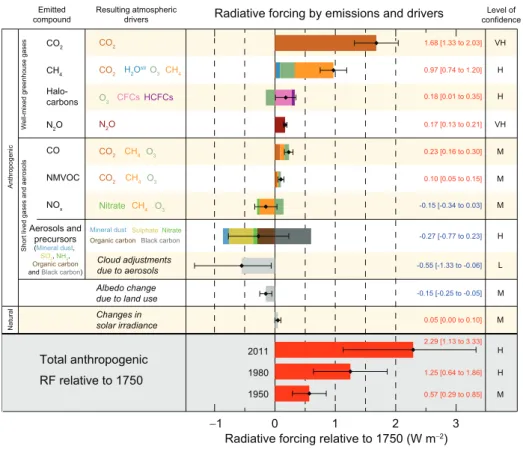
from black carbon absorption of solar radiation. There is high confidence that aerosols and their interactions with clouds have offset a substantial portion of global mean forcing from well-mixed greenhouse gases. They continue to contribute the largest uncertainty to the total RF estimate. {7.5, 8.3, 8.5}

• The forcing from stratospheric volcanic aerosols can have a large impact on the climate for some years after volcanic eruptions. Several small eruptions have caused an RF of –0.11 [–0.15 to –0.08] W m–2_{for the years 2008 to 2011, which} is approximately twice as strong as during the years 1999 to 2002. {8.4}

• The RF due to changes in solar irradiance is estimated as 0.05 [0.00 to 0.10] W m−2_{(see Figure SPM.5). Satellite} obser-vations of total solar irradiance changes from 1978 to 2011 indicate that the last solar minimum was lower than the previous two. This results in an RF of –0.04 [–0.08 to 0.00] W m–2_{between the most recent minimum in 2008 and the} 1986 minimum. {8.4}

• The total natural RF from solar irradiance changes and stratospheric volcanic aerosols made only a small contribution to the net radiative forcing throughout the last century, except for brief periods after large volcanic eruptions. {8.5}

Figure SPM.5 | Radiative forcing estimates in 2011 relative to 1750 and aggregated uncertainties for the main drivers of climate change. Values are global average radiative forcing (RF14_{), partitioned according to the emitted compounds or processes that result in a combination of drivers. The best} esti-mates of the net radiative forcing are shown as black diamonds with corresponding uncertainty intervals; the numerical values are provided on the right of the figure, together with the confidence level in the net forcing (VH – very high, H – high, M – medium, L – low, VL – very low). Albedo forcing due to black carbon on snow and ice is included in the black carbon aerosol bar. Small forcings due to contrails (0.05 W m–2_{, including contrail induced cirrus),} and HFCs, PFCs and SF6 (total 0.03 W m–2_{) are not shown. Concentration-based RFs for gases can be obtained by summing the like-coloured bars. Volcanic} forcing is not included as its episodic nature makes is difficult to compare to other forcing mechanisms. Total anthropogenic radiative forcing is provided for three different years relative to 1750. For further technical details, including uncertainty ranges associated with individual components and processes, see the Technical Summary Supplementary Material. {8.5; Figures 8.14–8.18; Figures TS.6 and TS.7}

Anthropogeni

c

Natura

l

−1 0 1 2 3

Radiative forcing relative to 1750 (W m−2₎

Level of confidence

Radiative forcing by emissions and drivers

1.68 [1.33 to 2.03]

0.97 [0.74 to 1.20]

0.18 [0.01 to 0.35]

0.17 [0.13 to 0.21]

0.23 [0.16 to 0.30]

0.10 [0.05 to 0.15]

-0.15 [-0.34 to 0.03]

-0.27 [-0.77 to 0.23]

-0.55 [-1.33 to -0.06]

-0.15 [-0.25 to -0.05]

0.05 [0.00 to 0.10] 2.29 [1.13 to 3.33]

1.25 [0.64 to 1.86] 0.57 [0.29 to 0.85]

VH H H VH M M M H L M M H H M CO2 CH4 Halo-carbons

N2O

CO NMVOC NOx Emitted compound Aerosols and precursors (Mineral dust, SO2, NH3,

Organic carbon

and Black carbon)

We

ll-mixed greenhouse gases

Short lived gases and aerosols

Resulting atmospheric drivers

CO2

CO2 H2OstrO3CH4

O3 CFCsHCFCs

CO2 CH4 O3

N2O

CO2 CH4 O3

Nitrate CH4 O3

Black carbon Mineral dust Organic carbon Nitrate Sulphate Cloud adjustments due to aerosols Albedo change due to land use Changes in solar irradiance

Total anthropogenic RF relative to 1750

1950 1980 2011

SPM

Figure 1.2: The change in the Earth’s radiative balance between the pre-industrial era (1750)

and the year 2011. Greenhouse gases (upper panel) have a clear warming effect, whereas

aerosols (third panel) are the major source of cooling. The uncertainty in the total radiative

forcing is dominated by the large error bars on the effect of aerosols. Figure from IPCC (2013).

on climate, cloud properties, and precipitation patterns, remain uncertain as particle concentrations, size, shape, and chemical composition are not measured with suffi-cient accuracy and spatial resolution to resolve their regional variety (IPCC 2013). Figure 1.2 shows the current knowledge of the global anthropogenic aerosol radia-tive forcing in terms of their direct and indirect effects; the cooling effect of aerosols, although significant in size, is highly uncertain compared to the warming effect of

greenhouse gases like CO2. Therefore, in spite of accurate long-term records of

tem-perature and greenhouse gases, there is a large uncertainty in the climate sensitivity through the uncertainty in the net change in radiative forcing, such that projections for global temperature change in the year 2100 vary by about 2

◦

(15)

1.2.3 Air quality

Exposure to particulate matter air pollution also has major adverse human health impacts, including asthma attacks, heart and lung diseases, and premature

mortal-ity (Anderson et al. 2011). Particulate matter smaller than 10 micrometer (referred

to as PM10) can enter the bronchi, and the smaller and lighter the particles are,

the deeper they can penetrate into the lungs. Chemical composition is believed to

play a significant role in toxicity; black-carbon (soot)-containing aerosols associated

with vehicular traffic appear to be particularly toxic. More accurate measurements

of aerosol size and chemical composition are needed to study the links between

pollution and public health.

1.2.4 Air traffic

Eruptions of the Islandic Eyjafjallajökull volcano in 2010 caused major air traffic dis-ruptions, leading to millions of stranded passengers, and an economic damage for

the air carriers of over a billion euros. Large parts of the European airspace were

closed for safety reasons, due to the damaging effect of ash particles on airplane

engines. According to new European guidelines, airplanes are still allowed to fly

in regions with ash concentrations below 2 mg/m

3

, which is about 3 orders of

mag-nitude more than usual (EASA 2013). Accurate concentration measurements with

large spatial coverage are needed to identify safe regions and reduce the air traffic downtime; characterization of the microphysical properties improves the forecasting of ash transport and dispersion.

1.3 Aerosol measurements

1.3.1 Particulate matter monitoring

To protect human health, governments set air quality standards, and monitor PM10

and PM2.5 levels. These are the most prevalent in-situ aerosol measurements, and

are performed in a standardized way. Air is sucked through sampling heads that

let particles pass that have a diameter smaller than 10 or 2.5 µm, respectively.

The accumulated particles are manually weighed according to the reference method, which is the official method for regulatory compliance and (inter)national comparison.

Instead of the expensive and time-consuming manual weighing, often automated

measurements are performed of the extinction of beta radiation by the contaminated

filter. These automated measurements have to be calibrated frequently using the

reference method. The filters can be analyzed in the laboratory to determine the

particles’ shape and chemical composition.

PM monitoring provides direct measurements of aerosol mass concentration in

two particle size groups at ground level, which is the most relevant location for

public health, on an hourly basis, but at a limited spatial coverage. For example,

(16)

rivm.nl_{) consists of about 60 monitoring stations in different scenes, for example}

rural areas, urban areas, close to traffic or close to industrial or agricultural activity, which is on average one per 700 square kilometers.

1.3.2 Sunphotometry

AERONET (Aerosol Robotic Network) is a global ground-based measurement net-work with about 400 stations in 50 countries on all continents, that is mainly used

for validation of satellite measurements (Holben et al. 1998). AERONET employs

sunphotometers to measure the extinction (i.e. scattering plus absorption) of direct

sunlight due to the total aerosol column. Although this aerosol optical thickness

(AOT) measurement itself is reliable, it cannot discriminate between the amount of aerosols and the intrinsic extinction capability (aerosol extinction coefficient) of that particular type of aerosols. The AOT is measured in a few spectral bands, to obtain a rough measure of aerosol size: the size of a particle relative to different wavelengths varies rapidly for small particles, and therefore the interaction is highly wavelength dependent, whereas large particles like water droplets exhibit a spectrally flat

be-havior. Empirical relationships between the AOT of the total aerosol column and

PM at ground level have been established, but the correlation remains weak (e.g. Schaap et al. 2009).

1.3.3 Lidar

Lidar is an active remote sensing technique, in contrast to the various passive tech-niques discussed in this thesis which use the Sun as light source. A lidar instrument

sends laser pulses into the atmosphere, and measures the arrival times and

in-tensities of the backscattered light. This results in altitude profiles of the aerosol

extinction coefficient. The use of multiple wavelengths gives an indication of

par-ticle size, and a depolarization measurement provides information on the aerosol

type (e.g. Murayama et al. 1999).

1.4 Light scattering and polarization

It is crucial for our understanding of the impact of atmospheric aerosols on climate and public health to be able to remotely characterize the physical properties of the

aerosols, in terms of size, shape and chemical composition. The information content

in the direct sun measurements is not large enough for that, and this technique

only works from the ground. The measurement dimensionality is greatly increased

by looking away from the Sun, to measure the sunlight that is scattered in the

atmosphere.

The physical mechanisms behind scattering depend on the sizedof the scatterer

(17)

in the order of nanometers, whereas aerosols and cloud droplets are in the order of

1–10µm, i.e. 4 orders of magnitude difference.

Rayleigh scattering is the re-radiation of incoming light in all directions by e.g. air

molecules withd << λ. To understand this, we should think of light as transverse

electromagnetic waves, consisting of an electric and a magnetic field, both oscillating perpendicular to each other and to the direction of propagation. When encountering a small particle, the electric field applies a force to the electrons inside the particle,

such that they start oscillating along with the electric field. This oscillating dipole

moment in turn emits radiation in all directions, except in the direction of oscillation,

i.e. along the dipole axis. This implies that the observed intensity depends on the

scattering geometry (location of light source, scattering particle, and observer) and the oscillation direction of the electric field, called the linear polarization direction, as depicted in Fig. 1.3.

A beam of light consists of many electromagnetic waves, that may have different polarization directions. In the most extreme case there is no preferred direction of the electric field, and the light is unpolarized, as is the case for the incoming sunlight. If

there is a net polarization, it is described by the angle of linear polarization (φL) and

the degree of linear polarization (PL), the fraction of the total intensity that is linearly

polarized. Figure 1.3 shows that a scattering event at larger angles increasesPL up

to 100% at a90

◦

scattering angle, while decreasing the intensity.

The reason why the sky is blue is the1/λ

4

wavelength dependence of the Rayleigh scattering efficiency, which is a factor 16 more efficient at 400 nm than at 800 nm. Rayleigh scattering is also responsible for red sunsets: on their long horizontal way

through the atmosphere, much more blue than red light gets scattered out of the

direct sunlight, leaving a red Sun.

Mie scattering applies for the d ≈ λregime, as is the case for cloud droplets

and aerosols. It is named after Gustav Mie, who derived exact expressions for the

intensity and polarization scattered by a spherical particle, by solving Maxwell’s

equations (Mie 1908). Extensions have been made to account for non-spherical

particles with various shapes (Mishchenko et al. 2000).

The scattering process is a combination of diffraction and reflection off the

par-ticle, refraction when entering or exiting it, and interference inside the particle. All

these effects exhibit different intensity and polarization properties, and different

de-pendencies on wavelength, scattering angle, particle size, and particle refractive

index, giving rise to characteristic scattering signals with high sensitivity to the

particle’s microphysical properties. For example, a rainbow is created at scattering

angles around138

◦

due to light that refracts when entering a droplet, gets reflected on the backside, and refracts again when exiting the particle, as shown in Fig. 1.4. The refraction angles are slightly wavelength dependent, due to dispersion of the

refractive index, which creates the color effect. In polarization, the rainbow shows

a distinct bump, as seen for Venus in Fig. 1.1a, where the exact angular position

depends on the particle size. Moreover, the width of the particle size distribution

determines the broadening and contrast of the rainbow polarization signal.

(18)

PHY232 - Remco Zegers - interference, diffraction & polarization 51

¾

certain molecules tend to

polarize light when struck by it

since the electrons in the

molecules act as little antennas

that can only oscillate in a

certain direction

Figure 1.3: Rayleigh scattering of light by air molecules. An unpolarized beam of light is incident from the left, depicted by different electric waves with different oscillation directions.

The molecule re-radiates in all directions, albeit only the electric field components that are

perpendicular to the direction of scattering. Hence, in the forward direction the scattered light

is brightest and unpolarized (PL= 0), whereas at90

◦

the light is fully polarized (PL= 1) at

p.347. Reprinted by permission of Pearson Education, Inc., Upper Saddle River, NJ.

Figure 1.4: The rainbow at a scattering angle of 138

◦

is caused by the refraction of

sun-light when entering and exiting a water droplet. It also has a characteristic polarization

(19)

10 Chapter 1

0 5 10 15

Effective Size Parameter

m = 1.3 m = 1.4

m = 1.5

m = 1.6

0 30 60 90 120 150 180 Scattering Angle (deg)

< 0.06 0.08 0.1 0.15 0.2 0.3 0.4 0.5 0.6 0.8 1 1.2 1.4 1.6 2 3 5 10 20 50 > Intensity [a.u.]

0 5 10 15

Effective Size Parameter

m = 1.3 m = 1.4

m = 1.5

m = 1.6

0 30 60 90 120 150 180 Scattering Angle (deg)

-100 -80 -60 -40 -20 000 20 40 60 80 100

Linear polarization [%]

Figure 1.5: Scattered intensity (upper) and degree of polarization (lower) for single scattering

of unpolarized incident light, as functions of scattering angle and effective size parameter

xeff = 2πreff/λ, for refractive indicesm varying from 1.3 to 1.6. The scattering particles are

spherical with a Gamma size distribution with an effective radiusreffand varianceveff= 0.2µm.

Figure adapted from Mishchenko & Travis (1997).

efficiency scales with 1/λ

2

), which is the reason why clouds are white. This also

causes a white aureole around the Sun, with a relatively large contribution of scat-tering by water droplets and aerosols, which decreases rapidly when moving away

from the Sun when Rayleigh scattering by small particles takes over. At the small

scattering angles close to the Sun, the light is refracted when entering and exiting the particle, which creates polarization in the plane of scattering, according to the

Fresnel equations. Note that this is perpendicular to the direction of polarization

due to Rayleigh scattering.

Figure 1.5 shows Mie scattering intensity and polarization for different refractive indices and effective size parameters. The latter is a combination of particle size and wavelength, reflecting the fact that measurements at multiple wavelengths provide information about the particle size. The polarization is more sensitive to the aerosol

microphysical properties than the scattered intensity, as it shows more variation

between the plots (different refractive indices), and more variation along the vertical axis (particle size).

(20)

wave traveling in thez-direction through timet, described by:

Ex(z, t) = E_x0exp [i(kz − ωt)] _(1.1) Ey(z, t) = Ey0exp [i(kz − ωt+δ)], _(1.2)

wherek is the wave number,ωis the angular frequency, andδis the phase delay of

they-component with respect to thex-component. At a fixed positionz, the electric

field vector traces a Lissajous figure in thex − y-plane over time, which depicts the

polarization state of that wave. For example, in the case thatδ= 0, the electric field

components are in phase, and a linear trace is obtained, i.e., the wave is linearly

polarized. For δ =π, the electric field components are exactly out of phase, such

that again a linear trace is obtained, albeit with its orientation mirrored around the

x-axis. In the special case thatEx0=Ey0 andδ=π/2, a circular trace is obtained,

so the wave is circularly polarized. In general the polarization state of a light wave

is elliptical.

This thesis deals with light scattered in the Earth’s atmosphere that is the inco-herent sum of many light waves with different polarization directions, and is therefore

only partially polarized. Hence, the Stokes formalism is used to describe the total

intensityI and the intensity and state of the polarized part of the light, according

to: S=     I Q U V     =     E2 x0+Ey20 E2

x0− Ey20

2E_x0Ey0cosδ

2E_x0Ey0sinδ

    =    

l+↔= _l + l =+

l − ↔ l − l

−     , (1.3)

where Q is the difference in intensity between the vertically and the horizontally

polarized components, U is the intensity difference between linear polarization at

±45◦_{, and}V _{is the intensity difference between right- and left-handed circular}

po-larization (Collett 2005).

In the case of light scattering in the Earth’s atmosphere, the degree of linear

polarization (PL) can be anything between 0 and almost 1, whereas the degree of

circular polarizationV /I is on the order of10

−4

(Kawata 1978). Therefore,

instru-ments like SPEX are optimized for measuring only intensity and linear polarization.

The degree (PL) and angle (φL) of linear polarization are related to the Stokes

pa-rameters, according to:

Q/I=P_Lcos 2φ_L, _(1.4a)

U/I=P_Lsin 2φ_L, _(1.4b)

i.e.:

PL=pQ2+U2/I, (1.5a)

φL=arctan2 (U/Q)/2. (1.5b)

Optical components that change the polarization state of light are described by

a4×4Mueller matrix, such that:

(21)

In the context of scattering, this Mueller matrix is called a scattering phase matrix. The general phase matrix for a collection of randomly oriented scattering particles,

as a function of scattering angleθ, is of the form:

Mscat(θ) =



  

M11(θ) M12(θ) 0 0

M12(θ) M22(θ) 0 0

0 0 M33(θ) M34(θ)

0 0 −M34(θ) M44(θ)



 

. (1.7)

In the case of isotropic, spherical scatterers,M11=M22 andM33=M44. The upper

left block represents the creation of polarization at±Q, i.e. parallel or perpendicular

to the scattering plane, whereas the lower right block describes the conversion of

linear polarization at45

◦

into circular polarization.

Scattering phase matrices are used extensively in radiative transfer algorithms to propagate Stokes vectors through a model atmosphere, to interpret multi-angle multi-wavelength measurements of intensity and polarization in terms of aerosol size,

shape, and chemical composition (Dubovik et al. 2006). The model atmosphere is

composed of thin plane-parallel layers, each containing a homogenous mixture of air

molecules and aerosols, bounded by a diffusely reflecting ground surface. For each

layer, the total transmission and reflection properties are calculated, and the layers are subsequently combined while taking into account multiple scattering between different layers, to obtain the intensity and polarization at ground level (Hasekamp & Landgraf 2002, 2005). When fitting the model to SPEX measurements, the free fit parameters are: aerosol optical thickness for large and small mode aerosols, aerosol particle size distribution for both modes, aerosol complex refractive index, aerosol

sphericity, and surface albedo. The real part of the refractive index is an indicator

for the aerosol chemical composition, as shown for the case of Venus in Fig. 1.1c. The imaginary part describes the amount of absorption by individual aerosols, which is an important parameter for detecting black carbon or soot.

1.5 Atmospheric scattering measurements

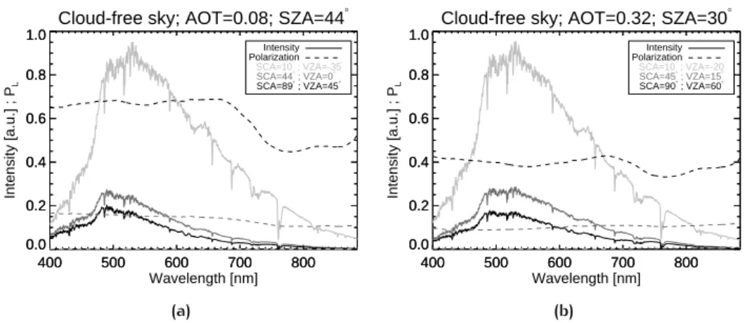
Examples of ground-based atmospheric scattering measurements, performed with

the groundSPEX instrument described in Chapter 5, are shown in Fig. 1.6. It shows

the intensity and degree of linear polarization PL of the cloud-free sky for three

different scattering angles: close to forward scattering, i.e. close to the Sun (10

◦

),

close to 90

◦

scattering, and at an intermediate angle. The angles are obtained by

pointing the instrument in different directions in the principal plane, which is the

vertical plane that goes through the Sun, zenith, and the instrument. This plane

provides the largest range of scattering angles, from 0–90◦ if the Sun is at zenith

to 0–180

◦

if the Sun is at the horizon. The scattered light is horizontally polarized,

because of the geometric principle depicted in Fig. 1.3.

The global shape of the intensity spectra is the black-body spectrum of the Sun.

(22)

400 500 600 700 800 0.0 0.2 0.4 0.6 0.8 1.0

Cloud-free sky; AOT=0.08; SZA=44°

400 500 600 700 800

Wavelength [nm] 0.0 0.2 0.4 0.6 0.8 1.0

Intensity [a.u.] ; P

L

Intensity Polarization

SCA=10° ; VZA=-35° SCA=44° ; VZA=0° SCA=89° ; VZA=45°

(a)

400 500 600 700 800

0.0 0.2 0.4 0.6 0.8 1.0

Cloud-free sky; AOT=0.32; SZA=30°

400 500 600 700 800

Wavelength [nm] 0.0 0.2 0.4 0.6 0.8 1.0

Intensity [a.u.] ; P

L

(b)

Figure 1.6: Measurements of the intensity and degree of polarization (PL) of a cloud-free sky,

with a small (a) and large (b) aerosol load. The instrument points at three viewing zenith

angles (VZA), to create scattering angles (SCA) close to 0, 45and90

◦

. The measurements

are taken with the groundSPEX instrument at CESAR Observatory, The Netherlands, on July

9, 2013. (a) 8:55 UTC. Solar zenith angle SZA=44◦. AOT=0.08 at 550 nm. (b) 11:41 UTC.

SZA=30

◦

. AOT=0.32 at 550 nm.

the absorption lines below 600 nm are Fraunhofer lines that originate in the solar atmosphere, whereas the broader absorption bands at longer wavelengths are mainly caused by oxygen and water vapor in the Earth’s atmosphere.

When looking away from the Sun, the intensity decreases, and PL increases, as

expected from Fig. 1.3. The intensity decrease is larger at longer wavelengths, which means that the sky gets an increasingly deep blue color when moving away from the Sun. This is the transition from white Mie with strong forward scattering to blue Rayleigh scattering.

The degree of polarization also shows a strong scattering angle dependence: it

goes from virtually 0 close to the Sun to 40–70%at90

◦

scattering. However, the

geo-metrical argument in Fig. 1.3 predicts aPL of 100% at90

◦

scattering. The significant depolarization is mainly caused by multiple scattering. If a lightwave gets scattered a second time, the scattering geometry is different, because the first scatterer acts as the light source. This deviating geometry can lead to a different angle of polariza-tion, and hence to depolarizapolariza-tion, because it dilutes the main polarization direction

due to single scattering. A second depolarizing factor is light that is diffusely

re-flected by the Earth’s surface, before it is scattered in the atmosphere towards the

instrument. This surface albedo effect is particularly noticeable when looking close

to the horizon, for example for a viewing zenith angle of VZA=45

◦

in Fig. 1.6a. The

strong decrease in polarization above 700 nm is due to the strong increase in re-flectance of vegetation in the infrared, called the red edge. The small dip at 550 nm

(23)

reason why PL < 1 at 90

◦

scattering is the intrinsic depolarization of anisotropic

gases, which for the diatomic air molecules leads to a maximumPL of 0.93 (Hansen

& Travis 1974). Finally, thin invisible clouds may be present with increased multiple scattering, leading to depolarization (Pust & Shaw 2008). The maximum polarization in Fig. 1.6b is much lower than in Fig. 1.6a due to the higher AOT and the larger VZA. The latter increases the optical path through the atmosphere and hence the multiple scattering, and the contribution of unpolarized ground reflectance increases closer to the horizon.

1.5.1 Current scattering instrumentation

Several instruments employ passive scattering measurements to determine the

at-mospheric aerosol load. They all have different numbers of viewing angles and

wavelengths, and most of them do not measure polarization, or with very limited

accuracy.

The AERONET sunphotometers, for example, also measure scattered light at a

large number of viewing angles, typically in four wavelength bands in the visible

part of the spectrum. This allows for the retrieval of particle size distribution, and

a rudimentary classification of the aerosols using the complex refractive index with an accuracy of 0.04 in the real part and 30% in the imaginary part (Dubovik et al.

2000). A new version of the sunphotometers including polarization measurements

at all wavelengths has become available. It has been shown that this instrument

indeed improves the retrieval of size distribution and refractive index (Li et al. 2009). In the end it is crucial to have satellites monitoring and characterizing

atmo-spheric aerosols, because of their large spatial and temporal coverage. Currently,

most global aerosol information comes from the MODIS instrument onboard the

Aqua and Terra satellites, and MISR onboard Terra, with AOT as their main

prod-ucts. MODIS (Moderate-resolution Imaging Spectroradiometer) employs intensity

measurements in 7 wavelength bands within 466-2119 nm for aerosol retrieval, and

is viewing in the nadir direction with a cross-track field-of-view of±55

◦

(Salomon-son et al. 1989, Remer et al. 2005). The lack of multiple viewing directions limits

the retrieval to a number of standard aerosol models. MISR (Multi-angle Imaging

SpectroRadiometer) measures intensities in four spectral bands within 446-866 nm,

in 9 along-track viewing directions within±70.5

◦

, with a cross-track field-of-view of

±14◦_{(Diner et al. 1998, Martonchik et al. 1998). These specifications, more similar to}

AERONET, allow for the retrieval of particle size distribution and complex refractive

index. The PARASOL/POLDER instrument, decommissioned in 2013 after 9 years

in orbit, combined multi-angle (16 angles within±43◦) multi-wavelength (443–1020

nm) imaging radiometry with polarimetry in 3 of the 9 spectral bands (Tanré et al.

2011). The additional polarization information, with an accuracy of ∼ 0.01−0.02,

greatly improves the retrieval of both macro- and microphysical aerosol

(24)

Waquet et al. 2013). The ability to retrieve cloud properties along with aerosols also results in much more usable data, because the scene does not have to be strictly cloud-free, and the quality of the aerosol retrieval depends less on the cloud screen-ing and residual cloud contamination, which is particularly interestscreen-ing in the twilight zone around clouds, the transition region from cloud droplets to dry particles.

To achieve a significant reduction of the uncertainty in climate sensitivity, an

understanding of the aerosol radiative forcing at the 0.25 W/m

2

level is required, through detailed and accurate aerosol characterization (Hansen et al. 1995, Schwartz 2004). The corresponding accuracies for macro- and microphysical aerosol properties have been derived (Mishchenko et al. 2004), and translated into measurement re-quirements (Hasekamp & Landgraf 2007, Hasekamp 2010), showing that sub-percent polarimetric accuracy is the key to success for the next generation angle

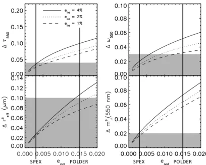
multi-wavelength polarimeters. As shown in Fig. 1.7, sufficiently accurate retrieval of the

important parameters of aerosol optical thickness and real refractive index (indicative of aerosol type and chemical composition) can only be achieved with a polarimetric

accuracy of ∼ 0.003. This is an order of magnitude better than the current

in-strumentation (Tanré et al. 2011), and requires groundbreaking concepts for both

the instrument and calibration. This is what we aim for with the development and

calibration of the SPEX instrument described in this thesis.

1.6 Measuring polarization

The intensity and linear polarization of light are described by 3 parameters:

in-tensity I, degree of linear polarization PL, and angle of linear polarization φL, or

equivalently, Stokes I, Q, and U. In fact, the definition of the Stokes parameters

in Eq. (3.2) provides direct instructions for measuring them using polarization filters

at different angles. For example, Stokes Q is the intensity transmitted through a

vertical polarizer minus that through a horizontal polarizer, i.e., Q =l − ↔. The

sum of the two intensities is the total intensity I, i.e.,I =l +↔, and Stokes U is

measured using a polarizer at45

◦

and−45

◦

, according toU = l − l . A rotating

polarizer is a common way of measuring linear polarization, and is used in Chapter 4 for calibration purposes.

The optics and detector behind the polarizer often exhibit polarization sensitivity,

such that rotation of the polarizer creates a spurious polarization signal. Therefore,

an alternative approach is to rotate or modulate the polarization in front of a fixed polarizer. The modulation is usually performed using a retarder that induces a phase

retardationδ between polarization along its ordinary (o) and extraordinary (e) axis,

according to:

δ= 2π∆n d

λ , (1.8)

where d is the thickness of the retarder, andλ is the wavelength of the light. The

(25)

SPEX POLDER SPEX POLDER

Figure 1.7:Uncertainty in retrieved aerosol parameters as a function of polarimetric accuracy: aerosol optical thickness (upper left), single scattering albedo (upper right), effective radius

small mode (lower left), real part of refractive index of small mode (lower right). The shaded

areas represent the requirements for climate research (Mishchenko et al. 2004). The vertical

lines represent the polarimetric accuracies of PARASOL/POLDER and SPEX. The calculations

are performed for radiometric accuracies of4%(solid line),2%(dotted line) and1%(dashed

line). The simulated satellite instrument has 17 along-track viewing angles within±60◦ and

10 spectral bands within350–2200nm. Figure based on simulations by Hasekamp (2010).

index for o and e polarization, which causes polarization dependent propagation

velocities, and hence a phase shift upon exiting. Waveplates, made of birefringent

crystals, such as quartz or magnesium fluoride, or stretched polymers, have a fixed birefringence at a fixed orientation. For example, half-wave plates mirror the angle of

incoming polarization around their axes by inducing a retardance ofδ=π, whereas

a quarter-wave plate with δ = π/2 converts circular into linear polarization and

vice versa. In order to modulate the polarization, several options exist to vary the

retarder ’s orientation or its retardance. For example, a rotating half-wave retarder

at0

◦

(vertical) and45

◦

, in front of a polarizer at0

◦

, provides a measurement of Stokes

Q, whereas rotation angles of22.5◦and−22.5◦ provideU. The axis of a ferroelectric

liquid crystal (FLC) can switch between two orientations by applying an alternating

electric field that rotates the long axes of the liquid crystal. In the case of a liquid

crystal variable retarder (LCVR), the retardance is tunable by applying an electric

field that tilts the long axes of the liquid crystal in the depth direction, thereby

reducing the anisotropy betweene ando. A photoelastic modulator (PEM) applies

(26)

We showed two intuitive examples of polarization measurements, using a rotating polarizer and a rotating retarder. In general, and more formally, the measured

inten-sity at modulation stateiis given by the dot product of the first row of the Mueller

matrix of the polarimeter at modulation state iand the Stokes vector under study,

as shown in Eqs. (3.2) and (3.5). Hence, a modulation matrixOcan be constructed,

consisting of the first rows of the Mueller matrices of themmodulation states, such

that the modulation process can be described as:         I1 I2 ... ... Im         =        

M1(11) M1(12) M1(13) M1(14) M2(11) M2(12) M2(13) M2(14)

... ... ... ...

Mm(11) Mm(12) Mm(13) Mm(14)

            I Q U V     in , (1.9) i.e.:

I=O S. _(1.10)

The measurements are demodulated afterwards using the demodulation matrix D,

according to:

S=D I, _(1.11)

whereDis the pseudoinverse ofO, i.e.:

D= OTO−1

OT. _(1.12)

It follows from Eq. (1.11) that the propagation of measurement noise to the Stokes parameters is determined by the magnitudes of the demodulation matrix elements.

This leads to the definition of the polarimetric efficiency for theith Stokes parameter,

according to (del Toro Iniesta & Collados 2000):

εi =



m

m

X

j=1 Dij2





−1_/2

, (1.13)

which is an important metric in polarimeter design. Maximization of polarimetric

efficiency is equivalent to the maximization of the modulation amplitudes for the

different Stokes parameters.

Remote aerosol characterization requires only linear polarimetry, i.e. the

mea-surement of I, Q and U. This can be achieved using a linear polarization filter

(polarizer) at different orientations. The Mueller matrix of a polarizer at0

◦

is given by:

Mpol=

1 2    

1 1 0 0 1 1 0 0 0 0 0 0 0 0 0 0



 

(27)

and it can be rotated over an angleφ around the optical axis according to:

M(φ) =R(−φ)M R(φ) ;R(φ) =



  

1 0 0 0

0 cos 2φ sin 2φ 0 0 −sin 2φ cos 2φ 0

0 0 0 1



 

. (1.15)

Hence, the modulation and demodulation matrix corresponding to a polarizer at0

◦

and90

◦

, and45

◦

and−45

◦

, are given by:

O= 1

2



  

1 1 0 0 1 −1 0 0 1 0 1 0 1 0 −1 0



  

;D=1 4



  

1 1 1 1 2 −2 0 0 0 0 2 −2 0 0 0 0



  

. (1.16)

The practical implementations for modulating polarization can be very different,

each having their advantages and disadvantages. This is reflected in the various

measurement concepts that are currently in development for remote aerosol

charac-terization. One of the main design choices is the dimension or domain in which the

modulation is performed:

• Temporal modulation. The recently decommissioned POLDER instrument

em-ploys a rotating filter wheel with polarizers at 0, 60 and 120

◦

to create the

different modulation states sequentially. Misregistration between successive

images, due to satellite motion during the ∼0.6 s modulation cycle, directly

translates into polarization errors. The main image shift is compensated using wedged prisms in the polarizer assembly (Hagolle et al. 1999), leaving a po-larimetric accuracy of 1% over the ocean to 2% over land, depending on spatial

gradients. The 3MI instrument, currently under development by CNES for the

MetOp (Meteorological Operational satellite) Second Generation programme of ESA and EUMETSAT, is based on the POLDER concept.

NASA supports the development and comparison of three polarimeter

con-cepts for its future ACE (Aerosol-Cloud-Ecosystem) mission: MSPI, APS and

PACS. The MSPI instrument employs temporal modulation at 25 Hz, using

pho-toelastic modulators with a rapidly oscillating retardance. At this frequency,

satellite motion is not an issue, but strict synchronization between the retarder

and detector is required to avoid mixing of modulation states. A polarimetric

uncertainty of<0.003has been demonstrated in the lab (Diner et al. 2010).

• Spatial modulation. The APS instrument, that failed to reach orbit in 2011,

employs pairs of identical telescopes with polarizers rotated by45◦ to

simul-taneously measure Stokes Q and U. Since each modulation state uses an

independent optical path and detector, polarimetric errors may arise from

dif-ferences in transmission and detector gain. APS uses single-pixel detectors

in combination with an along-track scanning mirror for multi-angle observa-tions, which allows for the use of an in-flight polarization calibration unit. The

(28)

PACS is a wide-field 2D imager, using a three-way polarizing beamsplitter to

image polarization at 0, 60, and120

◦

(optimal for linear polarimetry) onto three

independent focal planes. Preliminary calibration results show a polarimetric

accuracy of∼0.005(Buczkowski et al. 2013).

• Spectral modulation. SPEX, the instrument described in this thesis, employs a

static birefringent crystal and a spectrograph to encode the degree and angle of linear polarization as the amplitude and phase of a sinusoidal modulation

pattern in the intensity spectrum. This provides the full spectral intensity

and linear polarization information in a single shot, without moving or active

modulation optics (Snik et al. 2009). The most basic implementation of

spec-tral modulation is susceptible to aliasing between the specspec-trally modulated polarization and features in the incoming intensity spectrum with similar

spec-tral widths, such as absorption bands. The polarimetric accuracy of SPEX is

∼0.001 + 0.005· P_L_{, as demonstrated in Chapter 4.}

The most sensitive astronomical polarimeters combine temporal and spatial

mod-ulation to eliminate their intrinsic errors to first order, a technique called

beam-exchange polarimetry or spatio-temporal modulation (Semel et al. 1993, Bagnulo

et al. 2009). For example, a rotating half-wave retarder in front of a polarizing

beam-splitter rotates the incoming polarization, such that each polarization

direc-tion is measured twice: first the polarizadirec-tion is transmitted in beamAand blocked in

beamB, while in the second measurement the beams are exchanged. SPEX uses a

spatio-spectral version of beam-exchange polarimetry, where the two measurements are not separated in time, but shifted in wavelength, providing the same redundancy that eliminates intrinsic modulation errors, but in a snapshot fashion (see Chapter 6).

1.7 Polarimeter performance and calibration

Besides the modulation-specific errors, accurate polarimetry is hampered by a

va-riety of static and dynamic errors. Typical error sources inside a polarimeter are:

instrumental polarization due to differential transmission or absorption, depolariza-tion due to scattering, and crosstalk between different Stokes parameters due to,

e.g., misalignment or stress birefringence (Keller 2002). These errors may have a

dynamic component, e.g. due to temperature sensitivity. Moreover, intrinsically ran-dom errors are present, such as detector noise or in-flight contamination of the first

optical surface. The static errors are often much larger than the dynamic errors,

but after careful calibration the dynamic errors may dominate; imperfect calibration leaves residual static errors.

Each optical element in the polarimeter typically has several effects on the

po-larization, each described by a4×4Mueller matrix. Hence, it is almost impossible

(29)

parameters (de Juan Ovelar et al. 2011, Snik & Keller 2013). The approach in this

thesis for the error analysis of SPEX is the construction of a full Mueller matrix

model, followed by a realistic model of the polarimetric calibration. Monte Carlo

simulations on this end-to-end model, using realistic values for all error sources,

predict the complete polarimetric performance.

The purpose of polarimetric calibration is to find the modulation matrix that

relates measured intensities to the incoming Stokes vector, according to Eq. (1.10).

By applying different known polarization statesSusing a calibration stimulus, and

measuring the corresponding intensitiesI, one can solve for the modulation matrix

O_{. However, due to errors in the calibration measurements, and instrument changes}

after calibration, the modulation matrix and hence the applied demodulation matrix

are not perfect. Therefore, a measured Stokes vectorS0 differs from the true input

S_{, according to:}

S0=X S, _(1.17)

whereXis the4×4 response matrix (Ichimoto et al. 2007).

The main performance parameters of a calibrated polarimeter are its polarimetric

accuracy and sensitivity. The accuracy is the difference between the measured and

the true Stokes vectors, according to:

S0−S= (X−I4)S≡∆X S, (1.18)

where I4 is the4×4 identity matrix. In other words, a complete description of

ac-curacy is a4×4matrix∆X that describes the deviation from unity of the response

matrix. Polarimetric sensitivity describes the smallest measurable (change in)

po-larization, which is ultimately limited by detection noise, and obviously sets a lower limit to the polarimetric accuracy.

1.8 Brief history of SPEX

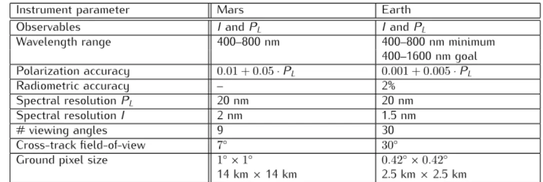
Even though SPEX, the Spectropolarimeter for Planetary EXploration, is currently focussing on the characterization of aerosols in the Earth’s atmosphere, the

instru-ment was originally designed in 2007 for studying massive dust storms on Mars

onboard the ExoMars Trace Gas Orbiter (Snik et al. 2008). A functional prototype

was developed in 2008–2010 by a Dutch consortium of academia and industry2,

according to the specifications in Table 1.1. Several calibration campaigns were

executed with the Mars prototype in the years following 2010, including the

cali-bration of polarimetric sensitivity and accuracy as presented in this thesis. In the

meantime, a design study was performed for the Europa Jupiter System Mission,

later called Jupiter Icy Moon Explorer, to fly SPEX in orbit around Jupiter to study clouds and haze particles, and Jupiter ’s moons Europa and Ganymede to study the

2

(30)

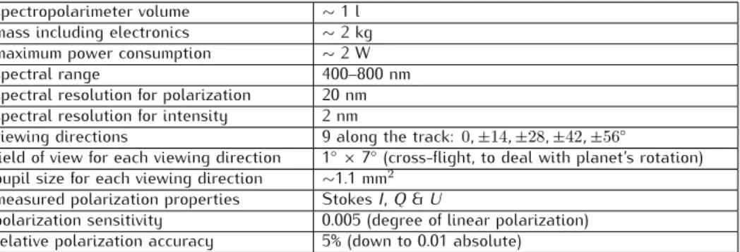
Instrument parameter Mars Earth Observables IandPL IandPL

Wavelength range 400–800 nm 400–800 nm minimum 400–1600 nm goal Polarization accuracy 0.01 + 0.05· PL 0.001 + 0.005· PL Radiometric accuracy – 2%

Spectral resolutionPL 20 nm 20 nm Spectral resolutionI 2 nm 1.5 nm # viewing angles 9 30 Cross-track field-of-view 7

◦ ₃₀◦

Ground pixel size 1

◦_×₁◦ ₀_.₄₂◦_×₀_.₄₂◦

14 km×14 km 2.5 km×2.5 km

Table 1.1: Typical specifications for a SPEX instrument for in-orbit characterization of the atmospheres of Mars and Earth.

composition and roughness of their icy surfaces. Radiation tests simulating Jupiter ’s strong radiation belts were successfully executed.

Soon it became clear that the performance of the prototype instrument exceeds the requirements for Mars, and SPEX was considered a good candidate for the more

stringent requirements for Earth observation (see Table 1.1). Earth observation is

more demanding, because it requires the simultaneous retrieval of a large variety

of aerosols, clouds, and the highly variable surface albedo. The more stringent

po-larimetric accuracy requirement is driven by the ability to discriminate between

different aerosol types via the refractive index (see Fig. 1.7). The large amount of

viewing angles is needed to sample the scattering phase matrix at the rainbow an-gles for detection of clouds and determination of the cloud droplet size distribution. This enables the characterization of aerosols near clouds, and reduces cloud

contam-ination in the retrieved aerosol parameters. The increased cross-track field-of-view

provides context around clouds and aerosol sources, and improves the spatial

cov-erage. An additional short-wave infrared channel improves the characterization of

coarse mode aerosols.

1.9 Thesis outline

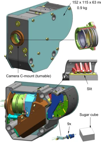
Chapter 2_{describes the SPEX instrument’s optical and mechanical design, and the}

realized prototype. Fundamental calibrations and data reduction steps are described that are necessary to convert raw detector images into intensity and polarization

spectra. In particular, the spectral polarimetric efficiency and its dependency on

the polarization angle is determined using a rotating polarizer, and interpreted. We

establish the2·10−

4

sensitivity of the polarimetric response of the SPEX prototype by supplying partially polarized light with slowly increasing degree of linear

polar-ization, using an increasingly tilted glass plate in front of a light source. Although

the absolute degree of polarization of this stimulus is not calibrated, fits to a Fresnel

(31)

for Mars of0.01+0.05·PL. We perform on-sky verification measurements, and provide

a qualitative interpretation. Moreover, the on-sky data led to various improvements

in the hardware and data reduction pipeline.

Chapter 3_{presents a comprehensive theoretical error analysis for spectrally}

mod-ulated polarimetry as implemented in SPEX. Various error sources are identified, and

classified according to their effect after calibration: static errors, such as

misalign-ments, decrease the measurement efficiency but do not impact thePL measurement

after calibration, whereas dynamic errors, e.g. due to temperature variations, directly

influence the measuredPL. Relevant dynamic effects for SPEX are in-flight

contam-ination of the first optical surface, temperature-induced variations in the multiple-order retardance, and spectrograph defocus due to thermal expansion, which directly changes the spectral modulation contrast on the detector, but the polarimetric

per-formance is limited by shot noise. We present an end-to-end model of an in-orbit

SPEX instrument, including static and dynamic errors and a realistic on-ground

calibration. We employ this model for Monte Carlo simulations of the in-flight

per-formance, showing that the probability of measuring the degree of linear polarization

with an error within±0.001(±0.002) is76% (99%) without in-flight calibration.

The results in Chapters 2 and 3 demonstrate the potential for reaching the

re-quired polarimetric accuracy of 0.01 + 0.05· PL with the SPEX prototype for Mars,

and even the 0.001 + 0.005· PL for Earth observation. The goal in Chapter 4 is

the experimental verification of the polarimetric accuracy of the SPEX prototype

at the challenging level of 10

−3

. The full data reduction pipeline of SPEX is

pre-sented first, and examples are shown of the demodulation of a fully and a partially polarized measurement. We subsequently present the constructed polarization

cali-bration stimulus: a carefully depolarized light source followed by two tiltable glass

plates to provide white calibration light to SPEX with a degree of linear

polariza-tion of0 .PL .0.5 at an accuracy of 0.001 + 0.005· PL. This accuracy cannot be

guaranteed by design over the entire PL-range due to uncertainties in the

polar-ization properties of the glass plates and their coatings. Therefore, a dual-beam

rotating analyzer verification polarimeter is constructed, and calibrated using both fully polarized light and the unpolarized output of the calibration stimulus, showing

a verification accuracy of 4·10

−4

. The stimulus zero-point is ∼ 10

−4

by design,

which is confirmed with SPEX in a direct PL measurement, as well as an indirect,

PL-independent method based on the measured rate of change of the angle of linear

polarization at small PL. The resulting difference between SPEX and the

verifi-cation polarimeter is smaller than 0.001 + 0.01· PL across the calibrated range of

0 _. P_L _. 0.5_. _However, _{after correction for a reproducible,} _{systematic deviation,}

the difference between the polarimeters is smaller than0.001 + 0.005· PL. The

po-larimetric accuracy of SPEX is suitable for the characterization of aerosols in the

Earth’s atmosphere. My contribution to this chapter is the design, construction and

(32)

Once the excellent polarimetric performance results of the SPEX prototype started trickling in, the Netherlands National Institute for Public Health and the Environ-ment (RIVM) expressed its interest in the developEnviron-ment of a ground-based SPEX

in-strument to investigate future air-quality monitoring networks. Chapter 5presents

the groundSPEX instrument that we developed, a low-cost, weatherproof SPEX in-strument on a motorized altazimuth mount for autonomous spectropolarimetric sky

measurements. We analyze the random and systematic errors in the radiometry

and polarimetry, and their propagation to the retrieved aerosol parameters. We

present the results of the four-day field-commissioning, in terms of AOT, particle

size, and refractive index, which are consistent with the co-located AERONET sta-tion. GroundSPEX is handed over to RIVM, which is commissioning it for permanent operation.

In Chapters 2–5 we have shown that the SPEX concept is suitable for

high-accuracy polarimetry at a spectral resolution of∼20nm, which is crucial for remote

aerosol characterization. Chapter 6 introduces new functionalities enabled by the

unique and powerful combination of a spectrograph and dual-beam spectrally mod-ulated polarimetry. We make use of the fact that the sum of the orthogonally modu-lated spectra is the unmodumodu-lated intensity spectrum at the spectrograph’s intrinsic resolution. This prevents aliasing between the modulation pattern and spectral fea-tures in the incoming intensity spectrum, and hence greatly improves the accuracy

of both the radiometry and polarimetry. We show how differential transmission

be-tween the opposite spectra leads to residual modulation in the sum-spectrum, and provide an iterative algorithm for post-facto extraction and correction of the

differen-tial transmission from the measured spectra. This dynamic transmission correction

reduces the associated polarimetric error by orders of magnitude, and enhances the instrument’s long-term in-flight stability. We proof that the redundancy in the spatio-spectral modulation reduces the sensitivity to uncorrected dark signal and transmis-sion or gain changes by orders of magnitude with respect to a beam-splitting-only

polarimeter. We demonstrate the ability of measuring polarization at the

spectro-graph’s intrinsic resolution of ∼1 nm. We measure the spectral polarization of the

clear sky using the groundSPEX instrument, showingPL= 0.160±0.010in the

Oxy-gen A absorption band, compared to PL = 0.2284±0.0004in the continuum. This

high-resolution absorption band polarimetry, unique amongst the various concepts for high-accuracy polarimetry for satellite-based atmospheric aerosol characteriza-tion, provides crucial information on the aerosol vertical stratification.