Active Learning Query Selection with
Historical Information
Michael Davy
A thesis submitted to the University of Dublin, Trinity College
in fulfillment of the requirements for the degree of
Doctor of Philosophy
Declaration
I, the undersigned, declare that this work has not previously been submitted to this or any
other University, and that unless otherwise stated, it is entirely my own work. This thesis
may be borrowed or copied upon request with the permission of the Librarian, University of
Dublin, Trinity College. The copyright belongs jointly to the University of Dublin, Trinity
College and Michael Davy.
Michael Davy
Acknowledgements
First and foremost, I would like to thank my supervisor Saturnino Luz for his belief, support and guidance throughout my research. Without his advice and insight this thesis would not have been possible. I would like to thank all my friends, who have made the last few years a memorable and enjoyable experience. I would especially like to thank Derek Greene, Peter Byrne, Kenneth Bryan and Aisling Linehan for their help and advice in proof-reading this thesis. I would like to take this opportunity to thank P´adraig Cunningham for introducing me to the topic of machine learning and guiding me in the early stages of my research. Finally, I would like to thank my parents and family. I am exceptionally fortunate to have such a supporting and loving family and I dedicate this thesis to them.
Michael Davy
University of Dublin, Trinity College
Abstract
This work describes novel methods and techniques to decrease the cost of employing active learning in text categorisation problems. The cost of performing active learning is a combi-nation of labelling effort and computational overhead. Reducing the cost of active learning allows for accurate classifiers to be constructed inexpensively, increasing the number of real-world problems where machine learning solutions can be successfully applied. In this thesis we investigate strategies and techniques to reduce both computational expense and labelling effort in active learning.
Critical to the success of active learning is the query selection strategy, which is respon-sible for identifying informative unlabelled examples. Selecting only the most informative examples will reduce labelling effort as redundant and uninformative examples are ignored. The majority of query selection strategies select queries based on the labelling predictions of the current classifier. This thesis suggests that information from prior iterations of ac-tive learning can help select more informaac-tive queries in the current iteration. We propose
History-based query selection strategies, which incorporate predictions from prior iterations
of active learning into the selection of the current query. These strategies have been shown to increase the accuracy of classifiers produced using active learning, thereby reducing la-belling effort. In addition, History-based query selection strategies are very efficient since information is reused from previous iterations of active learning.
Contents
Abstract iv
List of Figures xi
List of Tables xiv
Associated Publications xvi
Chapter 1 Introduction 1
1.1 Motivation . . . 2
1.2 Contributions . . . 3
1.2.1 Information from Past Iterations . . . 4
1.2.2 Computational Efficiency for Active Learning . . . 5
1.3 Related work . . . 6
1.4 Thesis Layout . . . 7
Chapter 2 Text Categorisation 9 2.1 Introduction . . . 9
2.2 Background . . . 10
2.2.1 Expert Systems . . . 10
2.3 Automated Text Categorisation . . . 11
2.4 Pre-processing: Parsing . . . 12
2.4.1 Vector Space Model . . . 12
2.4.2 Weighting Schemes . . . 13
2.4.3 High-dimensional Data . . . 14
2.5 Dimensionality Reduction . . . 15
2.5.2 Feature Extraction . . . 17
2.5.3 Unsupervised Dimensionality Reduction . . . 18
2.5.4 Policy . . . 19
2.6 Classifier Induction Algorithms . . . 19
2.6.1 k-Nearest Neighbour (k-NN) . . . 20
2.6.2 Na¨ıve Bayes . . . 22
2.6.3 Support Vector Machine (SVM) . . . 23
2.6.4 Ensembles . . . 28
2.6.5 Multi-Class Classification . . . 30
2.7 PAC Learning Model . . . 31
2.8 Evaluation . . . 32
2.8.1 Data Partitioning . . . 32
2.8.2 Confusion Matrix . . . 33
2.8.3 Accuracy . . . 34
2.8.4 Precision and Recall . . . 34
2.8.5 F1 Measure . . . 35
2.9 Summary . . . 36
Chapter 3 Active Learning 37 3.1 Introduction . . . 37
3.2 Limited Training Data . . . 38
3.2.1 Cost of Labelling . . . 38
3.2.2 PAC Bounds . . . 39
3.3 Active Learning . . . 40
3.3.1 Canonical Active Learning Algorithm . . . 43
3.3.2 Source of Unlabelled Examples . . . 44
3.3.3 Granularity . . . 45
3.3.4 Stopping Criteria . . . 46
3.3.5 Oracle . . . 47
3.3.6 Summary . . . 48
3.4 Query Selection . . . 48
3.4.1 Random Sampling . . . 48
3.4.3 Uncertainty Reduction . . . 49
3.4.4 Version Space Reduction . . . 51
3.4.5 Incorporating Unlabelled Data . . . 54
3.4.6 Multiple Strategies . . . 57
3.4.7 Summary . . . 61
3.5 Evaluation . . . 62
3.5.1 Fixed Intervals . . . 62
3.5.2 Learning Curves . . . 62
3.5.3 Deficiency . . . 63
3.5.4 p-value Plot . . . 64
3.5.5 Confidence Intervals . . . 64
3.5.6 Semi-supervised performance metrics . . . 65
3.5.7 Summary . . . 65
3.6 Summary . . . 65
Chapter 4 Methodology and Baseline Analysis 67 4.1 Introduction . . . 67
4.2 Datasets . . . 67
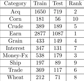
4.2.1 R10 . . . 68
4.2.2 20NG-4 . . . 69
4.3 Software . . . 72
4.3.1 Pre-processing . . . 72
4.3.2 Classification . . . 73
4.3.3 Active Learning . . . 73
4.4 Experiments in Active Learning . . . 74
4.4.1 Active Learning Components . . . 74
4.4.2 Parameters . . . 75
4.4.3 Evaluation . . . 76
4.5 Baseline Analysis . . . 77
4.5.1 Experiment Settings . . . 77
4.5.2 Results . . . 78
4.5.3 Discussion . . . 80
Chapter 5 History-Based Query Selection 82
5.1 Introduction . . . 82
5.2 Background . . . 83
5.3 History . . . 84
5.4 History-Based Query Selection . . . 85
5.4.1 History Uncertainty Sampling (HUS) . . . 86
5.4.2 History Kullback-Leibler Divergence (HKLD) . . . 87
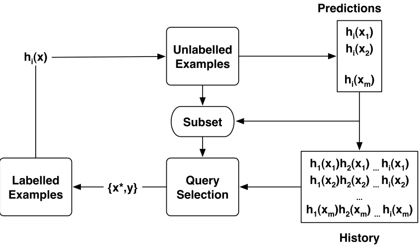
5.5 Filtered History-Based Query Selection . . . 88
5.5.1 Subset Construction . . . 89
5.5.2 History Uncertainty Sampling Filtered (HUSF) . . . 90
5.5.3 History Kullback-Leibler Divergence Filtered (HKLDF) . . . 90
5.6 Empirical Evaluation . . . 90
5.6.1 Preliminary Experiments . . . 91
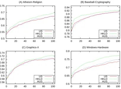
5.6.2 HUS . . . 92
5.6.3 HKLD . . . 96
5.6.4 HUSF . . . 99
5.6.5 HKLDF . . . 103
5.6.6 History Parameters . . . 105
5.6.7 Running Time . . . 107
5.7 Related Work . . . 109
5.8 Discussion . . . 109
5.9 Summary . . . 111
Chapter 6 Dimensionality Reduction for Active Learning 113 6.1 Introduction . . . 113
6.2 Background . . . 114
6.3 Unsupervised Dimensionality Reduction . . . 115
6.3.1 Document Frequency Global (DFG) . . . 115
6.3.2 Principal Components Analysis (PCA) . . . 116
6.4 Empirical Evaluation . . . 118
6.4.1 Experiment Settings . . . 118
6.4.2 Dimensionality . . . 120
6.4.4 Labelling Effort . . . 123
6.4.5 Fixed Stopping Criteria . . . 125
6.4.6 Random Feature Selection . . . 125
6.4.7 Supervised Dimensionality Reduction . . . 125
6.4.8 Alternative Classifiers . . . 126
6.5 Discussion . . . 128
6.6 Summary . . . 130
Chapter 7 Adaptive Pre-Filtering Error Reduction Sampling 131 7.1 Introduction . . . 131
7.2 Background . . . 132
7.2.1 Related Work . . . 133
7.3 Error-Reduction Sampling (ERS) . . . 134
7.4 Subset Optimisation . . . 137
7.4.1 Random Sub-sampling . . . 137
7.4.2 Pre-filtering . . . 137
7.4.3 Subset Size . . . 138
7.5 Adaptive Pre-filtering . . . 139
7.5.1 ERS-FPL . . . 139
7.5.2 Reward . . . 140
7.6 Empirical Evaluation . . . 141
7.6.1 Experiment Settings . . . 142
7.6.2 Error-Reduction Sampling . . . 143
7.6.3 Pre-Filtered ERS . . . 147
7.6.4 Subset Quality . . . 151
7.6.5 Adaptive Pre-Filtering . . . 153
7.6.6 Computational Expense . . . 156
7.6.7 Subset Size . . . 157
7.7 Discussion . . . 158
7.8 Summary . . . 160
Chapter 8 Conclusions 162 8.1 Introduction . . . 162
8.2.1 History-Based Query Selection . . . 163
8.2.2 Pre-Filtering Error Reduction Sampling . . . 164
8.2.3 Dimensionality Reduction for Active Learning Settings . . . 165
8.3 Thesis Contribution . . . 165
8.3.1 Computational Efficiency of Active Learning . . . 165
8.3.2 Incorporating Past Information . . . 166
8.4 Future Work . . . 166
8.4.1 Active Learning Performance . . . 166
8.4.2 Distributed Computing . . . 166
8.4.3 Early Stopping . . . 167
8.4.4 Alternative Domains . . . 167
Bibliography 168 Appendix A Supplemental Baseline Analysis Results 174 Appendix B Supplemental History-based Query Selection Results 177 B.1 HBQS . . . 177
B.2 Filtered HBQS . . . 177
B.2.1 Optimal Filtered HBQB . . . 188
List of Figures
2.1 CONSTRUE if-then-else rule . . . 11
2.2 Text Categorisation Overview. . . 11
2.3 Parsing . . . 12
2.4 Vector Space Model example . . . 13
2.5 Dimensionality Reduction . . . 16
2.6 Kernel Mapping . . . 24
2.7 SVM Classifier . . . 27
2.8 Data Partitioning . . . 33
2.9 Automated Text Categorisation System . . . 36
3.1 Passive Learning . . . 40
3.2 Active Learning . . . 41
3.3 Active Learning Toy Example . . . 42
3.4 Stream and Pool based Active Learning . . . 45
3.5 Learning Curves . . . 63
4.1 Data split for the R10 . . . 70
4.2 R10 Baseline Analysis . . . 78
5.1 History . . . 85
5.2 Filtered History . . . 89
5.3 Preliminary Results of HUS and HKLD on 20NG-4 with k-NN . . . 91
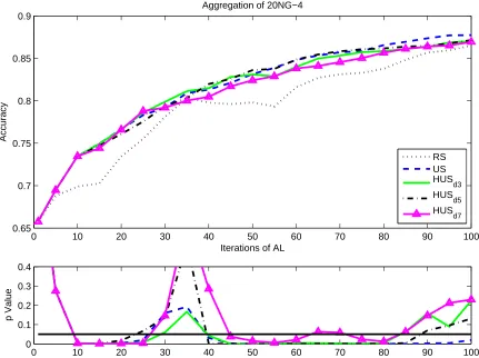
5.4 Aggregate Learning Curves for HUS on 20NG-4 . . . 93
5.5 Learning Curves for HUS on R10 . . . 94
5.6 Aggregate Learning Curves for HKLD on 20NG-4 . . . 97
5.8 Optimal HUSF and HKLDF Learning Curves for 20NG-4 . . . 100
5.9 Optimal HUSF and HKLDF Learning Curves for R10 . . . 101
5.10 Surface plot of the filtered History-based query selection parameters . . . 108
6.1 DFG aggressiveness on 20NG-4 . . . 121
6.2 DFG aggressiveness on R10 . . . 122
6.3 Learning Curves for Unsupervised Dimensionality Reduction on R10 . . . 122
6.4 Learning Curves for Unsupervised Dimensionality Reduction on 20NG-4 . . . 124
6.5 Learning Curves for Random Dimensionality Reduction on R10 . . . 126
6.6 Learning Curves for Supervised and Unsupervised Dimensionality Reduction on 20NG-4 . . . 127
6.7 Learning Curves for Alternative Classifiers on R10 . . . 128
7.1 Learning Curves for ERS-RS on 20NG-4 . . . 145
7.2 Learning Curves for ERS-RS on R10 . . . 146
7.3 Learning Curves for Pre-Filtering on 20NG-4 . . . 149
7.4 Learning Curves for Pre-filtering on R10 . . . 151
7.5 Learning Curves for Subset Comparison on R10 . . . 152
A.1 Baseline Analysis Learning Curves on R10 . . . 175
A.2 Baseline Analysis Learning Curves on R10 . . . 176
B.1 Learning Curves for HUS on 20NG-4 . . . 178
B.2 Learning Curves for HKLD on 20NG-4 . . . 179
B.3 20NG-4 HUSW T10 Results . . . 180
B.4 20NG-4 HUSW T25 Results . . . 181
B.5 20NG-4 HUSW T50 Results . . . 182
B.6 20NG-4 HUSW T100 Results . . . 183
B.7 20NG-4 HKLDW T10 Results . . . 184
B.8 20NG-4 HKLDW T25 Results . . . 185
B.9 20NG-4 HKLDW T50 Results . . . 186
B.10 20NG-4 HKLDW T100 Results . . . 187
B.11 Surface Plots HUSF on 20NG-4 . . . 189
List of Tables
2.1 Commonly used Kernels. . . 25
2.2 Confusion Matrix . . . 34
4.1 R10 category distribution . . . 68
4.2 20NG-4 Sub-problems . . . 71
4.3 Baseline Labelling Effort on R10 . . . 79
5.1 History Uncertainty Sampling Example . . . 87
5.2 Deficiency Values for HUS on 20NG-4 . . . 95
5.3 Deficiency Values for HUS on R10 . . . 95
5.4 Deficiency values for HKLD on 20NG-4 . . . 97
5.5 Deficiency Values for HKLD on R10 . . . 99
5.6 Deficiency values for HUSF on the 20NG-4 . . . 102
5.7 Deficiency values for HUSF on the R10 . . . 102
5.8 Deficiency values for HKLDF on the 20NG-4 . . . 104
5.9 Deficiency values for HKLDF on the R10 . . . 104
5.10 Deficiency values for HUSF on the 20NG-4 . . . 106
5.11 Deficiency values for HUSF on the R10 . . . 106
5.12 Deficiency values for HKLDF on the 20NG-4 . . . 106
5.13 Deficiency values for HKLDF on the 20NG-4 . . . 107
6.1 Dimensionality of Each Representation . . . 120
6.2 Labelling Effort for Unsupervised DR on R10 . . . 123
6.3 Labelling Effort for Unsupervised DR on 20NG-4 . . . 125
7.1 Confidence Intervals for ERS-RS on 20NG-4 . . . 144
7.3 Confidence Intervals for ERS-RS on R10 . . . 146
7.4 Deficiency for ERS-RS on R10 . . . 147
7.5 Confidence Intervals for Pre-Filtering on 20NG-4 . . . 148
7.6 Deficiency for Pre-Filtering on 20NG-4 . . . 150
7.7 Confidence Intervals for Pre-Filterting on R10 . . . 150
7.8 Deficiency for Pre-Filtering on R10 . . . 151
7.9 Rank for Subset Construction Techniques Deficiency Value . . . 155
Associated Publications
Davy, M. & Luz, S. (2007a). Active learning with History-based query selection for text cate-gorisation. Proceedings of the 29th European Conference on Information Retrieval Research, ECIR 2007 , 4425, 695.
Davy, M. & Luz, S. (2007b). Dimensionality reduction for active learning with nearest neighbour classifier in text categorisation problems. Proceedings of the 6th International Conference on Machine Learning and Applications (ICMLA07).
Chapter 1
Introduction
This thesis investigates methods and techniques to lower the cost of applying machine learning solutions using active learning. The cost of constructing an accurate classifier in an active learning setting is a combination of the number of labels required and the computational expense of performing active learning:
Cost = Labelling effort + Computational overhead
In this thesis we investigate two fundamental ways to reduce cost of active learning. First, we investigate ways to reduce the labelling effort. The critical component of active learning is the query selection strategy, which is responsible for identifying informative unlabelled examples. Selecting only the most informative examples will reduce labelling effort as redundant or uninformative examples are ignored. We investigate ways to select more informative queries by incorporating information from prior iterations into the query selection process. Secondly, we investigate ways to reduce the computational overhead. Many of the most successful query selection strategies require considerable computational overhead to select informative unlabelled examples. Practical solutions to reduce the computational expense in applying active learning are also investigated. We examine optimisation techniques for computationally expensive query selection strategies and unsupervised dimensionality reduction techniques.
1.1
Motivation
Categorisation is an integral part of human nature. Most humans find it difficult to extract information from unstructured data. By applying structure to data, information can be retrieved easily and efficiently. Perhaps the best example of the application of structure to data is exemplified through biological taxonomy. In recent years the production and storage of textual data has increased dramatically. Efficient automatic categorisation systems are required since the scale of the data produced renders manual categorisation impractical.
A first approach (Hayes & Weinstein, 1990) was a rule-based expert system with hand-crafted rules constructed by a dedicated team of domain experts. This approach required considerable effort to implement; however, it produced accurate classifiers which success-fully met the requirements of the problem. A serious limitation of hand-crafted rules is the
knowledge acquisition bottleneck (Sebastiani, 2002), whereby to redeploy the system to a new
domain, a new set of hand-crafted rules need to be produced, incurring considerable time and expense.
Machine learning offers a solution to the knowledge acquisition bottleneck through super-vised learning. Accurate text categorisation systems can be induced from a set of training data consisting of labelled examples. The task of hand-crafting rules was replaced by the much easier task of labelling examples. Training data are constructed by labelling a large sample of unlabelled examples drawn at random from the underlying data distribution. The probably approximately correct (PAC) learning model (see Section 2.7) places a bound on the number of labelled examples required to induce an accurate classifier for a particular concept. However, in practice, training data supplied to supervised learning process typically contains many times more labelled examples than is strictly necessary in order to guarantee the production of an accurate classifier. Supervised learning lowered the cost of construct-ing automated categorisation systems and propelled the widespread use of machine learnconstruct-ing solutions in many domains, allowing for considerable savings and increased productivity.
can be collected in a few hours; however, acquiring labels for all those webpages would take considerable time and effort. Employing supervised learning in such domains is impractical since there are insufficient training data to ensure that an accurate classifier is produced and the cost of producing enough training data outweighs the potential benefit of the solution.
A machine learning technique known as active learning (Angluin, 1988; Lewis & Gale, 1994) offers a possible solution to the label acquisition bottleneck. Active learning is a technique which can significantly reduce the number of labelled examples required to induce an accurate classifier. It does so by controlling the training data and labelling only the most informative examples. The difference in the number of examples (m) required to construct an accurate classifier as specified by the PAC learning model and the number of examples (N) supplied to supervised learning in practice can be quite large, with m ≪ N. Training data can contain many redundant and irrelevant examples which represents a considerable waste in labelling effort especially if the cost of acquiring labels is high. Active learning attempts to label only themmost informative examples. Significant reductions in the amount of labelled data required to produce an accurate classifier has been reported in the literature (Lewis & Gale, 1994; Tong & Koller, 2001).
Central to the success of active learning is thequery selection strategy which is responsible for identifying informative examples in the pool. The primary focus of this thesis is to improve the query selection process, either by incorporating information from previous iterations to help select more informative examples or by reducing the computational overhead of applying certain query selection strategies.
Active learning is a way to significantly reduce the cost of applying a machine learning so-lution. Contributions made in this thesis allow for further savings to be made when producing an accurate classifier using active learning. Reduced costs of deployment could potentially expand the number of domains in which machine learning solutions can be applied.
1.2
Contributions
learn-ing can be very computationally expensive. We investigate practical issues for lowerlearn-ing the computational overhead of performing active learning.
1.2.1 Information from Past Iterations
Active learning is an iterative process whereby in each iteration, information such as predic-tions on the remaining unlabelled examples are produced. This potentially valuable infor-mation is commonly discarded at the end of each iteration. We hypothesise that inforinfor-mation from past iterations of active learning can help select more informative examples in the cur-rent iteration.
History-based Query Selection
The majority of query selection strategies in the literature base the selection of the query on the predictions from the most recent classifier. These strategies are Markovian, in that the selection of a query in the current iteration is conditional only on the current classifier. The classifier and predictions produced in each iteration of active learning are ephemeral, that is, once the query is selected, the predictions are discarded.
We hypothesise that some potentially valuable information, which could help select in-formative unlabelled examples, is being lost. We investigate non-Markovian query selection strategies that incorporate predictions from past iterations of active learning into the selection of queries in the current iteration.
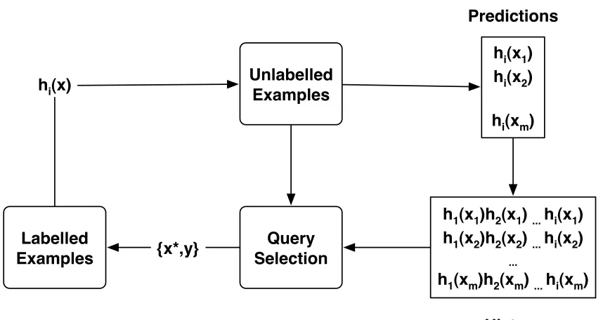
A data structure called History is used to capture all predictions on the unlabelled data produced in every iteration of active learning. History-based query selection strategies are developed which utilise the History to select unlabelled examples based on both the current and past predictions. Empirical evaluations show that incorporating History information into the query selection process, more informative examples are selected as queries, increasing the accuracy of the classifier produced and reducing labelling effort.
Adaptive Pre-Filtering
1.2.2 Computational Efficiency for Active Learning
Performing active learning can consume considerable computational resources. Reducing the computational overheads of active learning will subsequently reduce the cost of producing an accurate classifier, allowing machine learning solutions to be applied to many more domains.
Pre-Filtering Error Reduction Sampling
The computational overhead of employing error reduction sampling (Roy & McCallum, 2001) is directly proportional to the number of unlabelled examples it must consider as potential queries. Subset optimisation has been suggested as a way to reduce the computational over-head by restricting the number of candidate queries considered.
The most common way to construct the subset is random sub-sampling. We investigate
pre-filtering, where a query selection strategy is used to filter informative unlabelled examples
from the pool to form the subset. Pre-filtering is empirically evaluated as a way to both decrease the computational expense of error reduction sampling and simultaneously improve the quality of queries selected using error reduction sampling.
Empirically it is shown that pre-filtering can result in more accurate classifiers compared to random sub-sampling. Furthermore, pre-filtering using uncertainty sampling allows for smaller subsets to be used without decreasing the accuracy of the resulting classifier.
Dimensionality Reduction for Active Learning
Natural language text results in high-dimensional data when parsed into the vector space model. High-dimensional data is a problem since it increases both computational and storage overheads. Furthermore, some classifiers perform poorly in high-dimensional data due to
the curse of dimensionality. Dimensionality reduction techniques are commonly applied to
1.3
Related work
There has been substantial research into the problem of query selection. Chapter 3 discusses in detail some of the query selection strategies pertinent to the research in this thesis.
Chapter 5 investigates novel non-Markovian History-based query selection strategies, which incorporate information from prior iterations of active learning into the query se-lection process. Typically, query sese-lection strategies have based the sese-lection of queries on the predictions from the most recently induced classifier. Roy & McCallum (2001) discussed First order Markov active learning, where the aim is to select a query (x∗) such that, when
labelled and included in the training data, it will result in lower error than any other potential query.
It could be argued that History-based query selection strategies incorporate information about the unlabelled examples by utilising predictions from prior iterations. Query selection strategies discussed in Section 3.4.5 also incorporate information about unlabelled examples into the query selection process. However, such strategies incorporate unlabelled data di-rectly, while History-based query selection strategies incorporate the information indirectly via predictions. In addition, query selection strategies which incorporate unlabelled informa-tion are generally computainforma-tionally expensive. Error reducinforma-tion sampling (Roy & McCallum, 2001) for example has a time complexity of O(n2). The use of History makes it very efficient
to incorporate extra information about the unlabelled data.
Chapter 7 investigates pre-filtering as a way to reduce the computational overhead of performing error reduction sampling (Roy & McCallum, 2001). Culver et al. (2006) have previously used pre-filtering in error reduction sampling experiments. However, we extend the comparison both in terms of scale and techniques considered. Furthermore, the proposed adaptive pre-filtering technique is an extension of adaptive query selection strategies (Baram
et al., 2004; Pandey et al., 2005; Donmez et al., 2007). Adaptive query selection strategies
1.4
Thesis Layout
The remainder of this thesis is as follows:
Chapter 2 provides an overview of automated text categorisation. Various components of an automated text categorisation system are discussed including: parsing, dimension-ality reduction, classifier induction and evaluation. The PAC model, which gives a bound on the number of labelled examples required to induce an accurate classifier, is also discussed.
Chapter 3 reviews active learning, giving details on each component of the active learning process. The critical component of an active learning algorithm is the query selection strategy, which is responsible for the selection of informative examples from the pool. Query selection techniques which have emerged in the literature are reviewed.
Chapter 4 provides details on methodology of experiments conducted including datasets, classification algorithms and evaluation metrics used in the empirical evaluation. Base-line analysis provides motivation for active learning by demonstrating the benefit in reducing labelling effort.
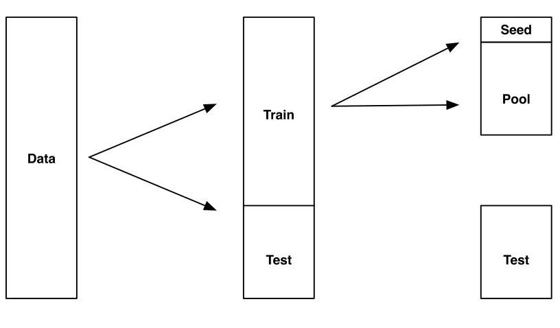
Chapter 5 introduces History-based query selection which incorporates predictions from classifiers in previous iterations of active learning into the selection of informative unla-belled examples from the pool. Predictions from the classifier induced in each iteration of active learning on the unlabelled examples are collected and stored in a data struc-ture called History. Non-Markovian query selection strategies are then developed which incorporate the information from the History into the selection of queries in the current iteration.
Chapter 6 discusses dimensionality reduction for an active learning setting. The major-ity of data supplied to an active learner is unlabelled; therefore, the most commonly used dimensionality reduction technique used in text categorisation, namely supervised feature selection, cannot be readily employed. We suggest the use of unsupervised dimensionality reduction techniques and empirically show how they benefit a k-NN classifier.
adaptive pre-filtering technique is proposed which can dynamically switch between fixed pre-filtering techniques.
Chapter 2
Text Categorisation
2.1
Introduction
Classification is the task of separating data into categories defined byconcepts that represent topics of interest. A text classification system assigns natural language documents to a set of predefined categories. Manual classification of documents is feasible for small amounts of data, however, due to the rapid growth in the production and storage of natural language documents manual categorisation has become impractical.
Automated text classification systems have emerged to solve this problem. Since their introduction in the 1980s they have evolved as new advances in machine learning have been proposed. The main motivation for continued research has been the reduction in effort to construct the automated systems.
2.2
Background
Classification is the task of assigning labels to data depending on whether or not they match a particular concept. Concepts are usually denoted by a label which can be used to categorise the data. For example if the input domain is e-mail and a message matches the concept of spam, it is assigned with “spam” label to signify its membership of this category.
More formally, given some input domain (X) and a set of labels (Y), a classifier can be viewed as a Boolean-valued function which maps from input to labels according to some concept, thereby assigning membership to a particular category. The target function (f :
X 7→ Y) always maps from input documents to their correct labels. The goal of automated text classification is to construct a hypothesis (h : X 7→ Y) which approximates the target function as closely as possible.
The manner in which the hypothesis is constructed has evolved over time, however, the objective of constructing a function, which approximates as closely as possible to the target function, remains the same.
2.2.1 Expert Systems
The first successful solution to the problem of automated text classification was delivered through expert systems in the 1980s. Expert systems consist of a series of hand-crafted rules constructed by dedicated domain experts. These rules form the hypothesis (h:X →Y) and are used to classify previously unseen documents.
The CONSTRUE system (Hayes & Weinstein, 1990) is a well-documented example of a successful expert system. Domain experts constructed rules which classified documents based on words that occurred within them. An example rule is shown in Figure 2.1.
CONSTRUE was a major success achieving high levels of performance, practically match-ing precision and recall levels of human indexers. Its deployment saved millions of dollars and significantly reduced the time taken to classify documents.
if
then WHEAT else (¬ WHEAT)
("wheat" & "farm") or ("wheat" & "commodity")
("bushels" & "export")
or or or ("wheat" & "tonnes")
("wheat" & "winter" and (¬ "soft"))
Figure 2.1: An if-then-else rule from CONSTRUE. For example, this rule assigns the label WHEAT to a document which contains the word “wheat” and the word “farm”. Documents for which the conditions are not met are assigned the label ¬WHEAT
2.3
Automated Text Categorisation
Machine Learning offers a solution to the knowledge acquisition bottleneck through the use of classifier induction algorithms, which learn a particular concept automatically from a set of positive and negative examples of the concept. This eliminates the burden of requiring domain experts to manually construct a hypothesis using hand-crafted rules and replaces it with the far less expensive task of labelling a set of examples.
Automated Text Categorisation (ATC) is a machine learning solution to the problem of classifying natural language documents. These techniques employ induction algorithms to construct classifiers from a set of examples labelled according to the concept to be learned. Supplied with training data consisting of positive and negative examples of the concept, the induction algorithm must produce a classifier that accurately classifies unseen examples.
An ATC system is comprised of a series of processes. Figure 2.2 shows how these sub-processes interact to deliver a classifier capable of accurately classifying new and previously unseen examples.
Evaluation Classifier
Induction Preprocessing
We give a brief overview of each element in an ATC system, ranging from pre-processing to evaluation metrics used to asses the quality of the classifier produced. Text categorisation is a very broad topic encompassing many disciplines. In this thesis we give details only for those aspects of text categorisation that are pertinent to our research. The interested reader is directed to (Sebastiani, 2002; Mitchell, 1997) for a full description of automated text categorisation and machine learning techniques.
2.4
Pre-processing: Parsing
Induction algorithms do not have the ability work directly with real world objects; rather they work on models, which represent real world objects. Even machine-readable document formats such as XML and PDF require transformation into an appropriate model before use with classification induction algorithms.
Parsing is the process whereby document attributes are extracted from the original raw representation and stored in a new internal representation, which can be easily interpreted by classification induction algorithms. This process is depicted in Figure 2.3
Parsing
VSM
Attributes
Documents
Figure 2.3: Parsing. Information from raw text documents in encoded in the Vector Space Model (VSM) which classifier induction algorithms can interpret. The VSM can be seen as a document Xattribute matrix where documents are represented by the rows and attributes are represented by the columns.
2.4.1 Vector Space Model
matrix is formed by stacking the document vectors.
Documents are described by their attributes, which can be any information about a docu-ment. A common approach for text classification is for attributes to represent the text within the document. The most straightforward approach is the bag-of-words (BOW) representa-tion, where documents are considered to be an unordered set of words. Documents are parsed into their individual words (tokenised) and frequency information is recorded in a vector of length |τ|with the vocabulary (τ) containing all possible words in the corpus.
Attributes correspond to the words and their values represent the frequency of the word within the document. All position and structural information about the occurrences of the words are ignored. Despite this disposal of potentially beneficial information the BOW rep-resentation works very well and it is the de-facto standard in text classification.
"a b a c d"
h
1 f
d d1
1
1 1
2
e c
1
d3
2
1 2 1
a
1 1
1 b
d2 "b c d c f f"
"h f b a d"
Figure 2.4: Vector Space Model (VSM). Each document is encoded in the VSM as a vector where each element represents the frequency of each attribute in the document. For example, the attribute “a” occurs twice in documentd1, once in d3and not at all ind2
Increasingly sophisticated representations can be achieved by changing what constitutes an attribute. For example, n-grams consider an attribute to be a phrase rather than a word. This allows some ordering information to be retained. However, new problems arise as the vocabulary size dramatically increases. Dumais et al. (1998) suggest that the addition of
n-gram terms actually decreases the overall performance of classification systems.
2.4.2 Weighting Schemes
As testament to the influence of Information Retrieval (IR) in machine learning, term weigh-ing schemes (Salton & Buckley, 1988) are commonly used. Term weights were developed for use with the vector space model as a means to adjust the influence of certain attributes. There are three components to a weighting scheme:
within individual documents. Binary weighting simply represents the absence or pres-ence of a term in a document by a 0 or 1 respectively. Terms that occur more frequently in a document should be considered more important, hence given a higher weight. Term frequency (tf) measures the number of times a term (wi) occurs in a document (dj).
tf(wi, dj)
Collection Component. The collection component of the weighting scheme allows us to adjust the influence of a term. The document frequency of a term is the number of documents it appears in within the corpus.
DF(wi)
By multiplying the term frequency by the inverse of document frequency (tf ∗idf), more influence can be given to terms which are frequent in a document but which are infrequent within all documents in the corpus (D).
tf ∗idf(wi, dj) =tf(wi, dj)∗log |D|
DF(wi)
Normalisation Component Finally the normalisation component allows for documents of different length to be given equal weight. L2 (cosine) normalisation is commonly used as shown in (2.1).
xi=
tf∗idf(wi, d)
q P|τ|
j=1tf∗idf(wj, d)
(2.1)
whereτ is the vocabulary. Weighting schemes range in complexity and generally have a large impact on the performance of the classification system.
2.4.3 High-dimensional Data
Text data is high-dimensional by nature. The principal causes of high-dimensional data in text stems from the richness and variety of natural language combined with the vector space model representation of documents.
sparse vectors, with the number of non-zero elements being quite low, as demonstrated in the example from Figure 2.4.
High-dimensional data increases computational expense. Comparisons between two fea-ture vectors requires examining all feafea-tures, therefore high-dimensional data requires in-creased computational expense. Similarly, memory and storage requirements are inin-creased in order to handle very large vectors and matrices.
Furthermore, induction algorithms are susceptible to thecurse of dimensionality (Mitchell, 1997), which loosely states: as the number of features increases, the performance of machine learning algorithms tends to decrease, sometimes significantly. Unlike information retrieval where matching algorithms scale well with very large numbers of features, classifier induction algorithms tend to suffer when supplied with high-dimensional data. The degradation in performance can be attributed to the presence of many irrelevant and redundant features in the data, which make the classification process all the more difficult. For example, classifi-cation algorithms such as the k-nearest neighbour (k-NN) that depend on similarity metrics are affected since examples from completely disparate topics can seem similar if they share a large number of these irrelevant features.
In an effort to reduce the overall number of terms to consider the Porter stemming algo-rithm (Porter, 1980) and stopword removal are sometimes used. Stemming is the collapsing of words to their common morphological root (e.g. “computers” and “computing” are stemmed to “comp”). Stemming sometimes reduces the effectiveness of classification systems hence there are times when it is not used. Stopwords are words that occur frequently in all docu-ments. These offer little information and waste storage resources. Removal of stopwords is straightforward; a list of common stopwords is kept and while documents are being tokenised, if a token matches a stopword it is discarded.
2.5
Dimensionality Reduction
After parsing is complete, the original data is represented by a set of attributes. The di-mensionality of this representation is typically very high. Didi-mensionality reduction is achieved by representing the original data using a small number of features as shown in Figure 2.5. A feature can be any attribute or a combination of multiple attributes and can either be selected or extracted from the original set of attributes describing the data. Here we make the distinction that the data is described by attributes after parsing while it is described using features after dimensionality reduction (if any) is performed. The number of features should be less than the number of attributes.
|features| ≪ |attributes|
Of course if no dimensionality reduction is performed, then the number of features will equal the number of attributes.
Dimensionality Reduction
VSM
Attributes
Documents
VSM
Documents
Features
Figure 2.5: Dimensionality Reduction for the VSM. After parsing the data is represented using a large number of attributes. Dimensionality reduction represents the same data using much fewer features with minimal loss of information.
Dimensionality reduction offers a host of benefits including reducing computational over-heads and sometimes increasing classifier performance (Yang & Pedersen, 1997). Given the benefits of dimensionality reduction it is commonly used as a pre-processing stage in ATC systems.
Features are found in two principled ways, namelyfeature selectionandfeature extraction. Feature selection is where a subset of the original attributes are used to represent the data. Feature extraction is where features are formed as combinations of one or more attributes.
2.5.1 Feature Selection
Many metrics have been proposed to evaluate the attributes. Empirical evaluation of the various metrics (Yang & Pedersen, 1997; Forman, 2003) has shown Information Gain to be one of the best performing. These studies have also shown that increased classification accuracy can be achieved when feature selection is applied. There are two principled methods to perform feature selection:
Filter-based methods seek to find the optimal subset of features irrespective of the classi-fication algorithm used. The original attributes are ranked with an appropriate metric (e.g. Information Gain) that defines how discriminative the attribute is. A subset of the most discriminative attributes are chosen to be the features according to a user-defined threshold.
Wrapper-based feature selection is where the selection method has explicit knowledge (and use) of the classification induction algorithm. Induced classifiers are used to help se-lect the optimal subset of attributes for the particular type of classification induction algorithm. While wrapper-based methods have the advantage of tailoring the feature selection to the classification algorithm, a major disadvantage is the computational overhead.
The simpler and computationally less expensive filter-based methods are far more preva-lent in text categorisation systems.
2.5.2 Feature Extraction
Feature extraction is an alternate approach for dimensionality reduction where the original data is represented by a succinct number of new features constructed from (combinations of) the original attributes. These new features are constructed in such a way that there is minimal loss of information.
More formally, PCA orthogonally transforms the coordinate system used to represent the data. The new coordinate system is defined by principal components which represent directions of maximal variance in the original data. Most of the information contained in the original representation can generally be represented using just a small number of principal components.
Principal components are the eigenvectors as given by the eigenvalue decomposition of the covariate matrix constructed from the centred data. Eigenvectors are ranked according to their associated eigenvalues, which signify the proportion of variance in the data accounted for by the eigenvector. Thus, the first principal component is the eigenvector with the largest associated eigenvalue, the second principal component is the eigenvector with the second largest associated eigenvalue and so on.
A small set of leading eigenvectors are selected which account for the majority of the variance and the original data is projected onto this subspace. The number of eigenvectors chosen is typically based on the proportion of variance in the data set accounted for by the chosen eigenvectors. If too few are chosen, reconstruction error will be high as the variance in the data was not well captured, similarly if too many are chosen the reduction in dimensionality can be low.
There are a number of drawbacks to PCA. The first is that features are no longer hu-man interpretable which can cause confusion in real world scenarios. Secondly eigenvalue decomposition on very large matrices is an expensive operation.
Finally, there are assumptions made in PCA, the most notable one being that the data is linearly separable. Kernel Principal Component Analysis (Sch¨olkopf et al., 1999b) was proposed which extends the ability of PCA to find non-linear transformations of the original data. Other feature extraction techniques used in machine learning include, Independent Component Analysis (Comon, 1994), Random Projections (Bingham & Mannila, 2001) and Local Linear Embedding (Roweis & Saul, 2000).
2.5.3 Unsupervised Dimensionality Reduction
2.5.4 Policy
The way in which a dimensionality reduction technique is applied is referred to as a policy. There are two distinct ways in which a dimensionality reduction technique can be applied, namely a global and local policy.
Local is where a reduced set of features are chosen for each individual category in isolation of other categories (Apt´eet al., 1994). Essentially this means that each document will have a separate representation for every category under consideration. Local dimensionality reduction is a context-sensitive method since category information is explicitly used.
Global is where a reduced set of features are chosen irrespective of the category under consideration (Yang & Pedersen, 1997). This is a context-free method of performing dimensionality reduction.
Most dimensionality reduction techniques can be applied in both a local and global policy. However, local dimensionality reduction assumes that label information is available. This assumption does not hold in an active learning setting and we explore this issue further in Chapter 6.
2.6
Classifier Induction Algorithms
In classification we wish to build classifiers for concepts, such as “is this e-mail a spam?”. Concepts correspond to a subsets of the input domain (X). For text classification, the goal is to build classifiers from a set of labelled examples that can automatically assign new documents to a set of predefined categories.
An alternative view of a concept is as a Boolean-valued functionf :X 7→ Y which decide membership of an input patterns to a concept. This function is referred to as the target
function, which always correctly labels input patterns.
Induction allows the learner to learn an approximation (hypothesis) of the target function from a limited amount of examples labelled by the target function. Generally more than one hypothesis can be induced from a given training set. The set of all hypotheses consistent with the observed training data is called the version space (Mitchell, 1997).
learn-drawn from the input space X and labelled using some unknown function y =f(x), an in-duction learning algorithm will output a classifierh(x) which is a hypothesis of the unknown target function f(x).
There is a vast number of classifier induction algorithms available. Detailed description of all classifiers is beyond the scope of this thesis. The remainder of this section gives an overview of each of the main classification induction algorithms used throughout the research conducted. We also discuss ensemble based approaches where multiple classifiers are used.
2.6.1 k-Nearest Neighbour (k-NN)
The k-NN classifier is perhaps one of most straightforward classification algorithms. It is an instance based classifier where new documents are assigned labels based on the closest training examples as given by a similarity metric. An assumption exists that examples of the same concept should be similar to each other.
In contrast to most classification algorithms which are eager (process their training data immediately) the k-NN is a lazy algorithm, delaying processing of training data until classi-fication time. See (Yang et al., 2003) for more details on running time.
For an input xq ∈X thek-NN will find the k training examples which are most similar
as defined by the similarity metric. Let S be the set of thekmost similar training examples, then, the predicted label for the input example is assigned to be the mode of the predictions of the nearest neighbours labels as shown in (2.2)
h(xq)←arg max
y∈Y
X
xi∈S
δ(y, f(xi)) (2.2)
where δ(a, b) equals 1 iff a = b otherwise 0. The similarity of the input xq and the most
similar training examples can be used to give finer control on the predicted class label as shown in (2.3). Here, more similar training examples have more influence in the predicted label.
h(xq)←arg max
y∈Y
X
xi∈S
sim(xq,xi)δ(y, f(xi)) (2.3)
the greater the distance the more dissimilar two feature vectors are.
d(xi,xj) =||xi−xj||=
v u u t
|τ|
X
l=1
(xil−xjl)2 (2.4)
While Euclidean distance works well for many types of machine learning problems, it sometimes works poorly with high-dimensional data common in text classification problems due to the curse of dimensionality. Two quite different documents might be deemed similar because they share a large number of irrelevant features. An alternative similarity metric commonly used in information retrieval tasks is cosine similarity (2.5). It defines similarity as the angle between two feature vectors. This metric can be used in place of Euclidean distance for the k-NN classifier, where neighbours are defined based on maximum similarity rather than minimum distance.
COS(xi,xj) = h
xi,xji
||xi|| · ||xj||
(2.5)
Predictions
The output of thek-NN can be transformed into a probabilistic classifier by considering the distance to each of the neighbours. Equations (2.2) and (2.3) can be modified to return the
weight of each predicted label. The weights are then normalised to give a pseudo-probabilistic
output from the classifier predictions.
Parameters
The choice of k is an important parameter. The most straightforward approach is to assign the label of the most similar training example, referred to as a 1-NN. Varying the value of
k will have an impact on the accuracy of the classifier. The optimal value for k is typically found using a validation set.
Performance
2.6.2 Na¨ıve Bayes
Probabilistic classifiers estimate P(Y|X) the probability of a label given a document. Given a new document to classify (x∈X) a Bayesian classifier will assign a label (y∈ Y) for which
P(y|x) is highest, as shown in (2.6).
ˆ
f(x) = arg max
y∈Y P(y|x) (2.6)
Induction algorithms must approximate the target function by estimating the probabil-ities based on observed training data. Bayes rule (Mitchell, 1997, Chapter 6) specifies how the conditional probability P(Y|X) can be constructed from observing training examples consisting of documents from each concept as labelled by the target function.
Using Bayes theorem (2.6) can be rewritten as:
h(x) = arg max
y∈Y P(y)
P(x|y)
P(x) (2.7)
Estimates of P(Y) are constructed from the training data by simply counting the fre-quency of the labels. However, estimating P(X|Y) is more challenging since there are poten-tially infinite variations of X. In order to obtain reliable estimates, the training data must contain multiple copies of every possible variation of X.
The na¨ıve Bayes classifier makes the assumption that attributes are conditionally inde-pendent. While this assumption is clearly false, significant simplifications in calculations can be made where (2.7) can be written as shown in (2.8):
h(x) = arg max
y∈Y P(y)
Y
xi∈x
P(xi|y) (2.8)
where P(xi|y) is the probability of a term for a given label and the denominator P(x) in
(2.7) is not computed since it is the same for all y ∈ Y.
Multinomial Na¨ıve Bayes
Throughout this thesis we concentrate on themultinomial variant of the na¨ıve Bayes classifier as used in (McCallum & Nigam, 1998). The multinomial na¨ıve Bayes assumes text documents are generated by a mixture model, parametrised by θ.
A classifier is induced by estimatingθfrom a set of labelled training data (Dℓ⊂X). The
occurs in a document of that category.
ˆ
θxi|y =
1 +P
x∈Dℓtf(xi,x)P(y|x)
|τ|+P|τ|
k=1
P
x∈Dℓtf(xk,x)P(y|x)
wheretf(xi,x) is the count of the termxi in the documentxandP(y|x) is the class label for
the training document x. Laplacian smoothing is used to avoid zero probabilities. Similarly, calculation of the probability of a category is simply the percentage of the training data that is of the same category.
ˆ
θy =
P
x∈DℓP(y|x)
|Dℓ|
Using these two estimates a classifier can be constructed where the predicted category is the label (y ∈ Y) with the highest probability and the probability of a label given a document (x) is calculated using (2.9):
P(y|x) = P(y| ˆ
θ)Q
xi∈xP(xi|y; ˆθ)
P
y∈YP(y|θˆ)
Q
xi∈xP(xi|y; ˆθ)
(2.9)
Performance
The na¨ıve Bayes classifier was popular for text categorisation tasks due to its simplicity and ease of implementation. Despite the strong independence assumptions made, the classifier performed well in text classification tasks. However, it has been shown (Yang & Liu, 1999) that its performance has been eclipsed by kernel methods classifiers such as the support vector machine.
2.6.3 Support Vector Machine (SVM)
In recent years kernel methods have been extremely popular due to their excellent per-formance on many machine learning tasks and in particular on text categorisation tasks (Joachims, 1997). Rather than devising a different algorithm for each domain, they settle on a standard set of algorithms and transform the data to a representation that suites the set of algorithms. Kernel methods consist of two modular components. The first is a standard classification algorithm, while the second is a kernel function that is used to transform the data to allow for easier classification using the classification algorithms.
Kernel
A classifier can easily be induced to correctly classify data from a domain which is linearly separable. However, for many real world problems the classes in the input space are unlikely to be linearly separable. One solution is to use a classifier specifically for each domain, e.g. using the non-linear classifier such as the k-NN. Kernel methods use an alternative strategy whereby the data is re-coded so that it becomes much easier to classify. A standard classification algorithm can therefore be used on all domains.
The function Φ(x) transforms (re-codes) the original input into a new feature space. Typically the dimensionality of the transformed feature space is much higher than the original feature space. Figure 2.6 shows an example where the data is non-separable in 2 dimensions but is separable in 3 dimensions. Explicitly transforming each input into the new feature space is computationally expensive (and potentially infeasible when infinite dimensions are used).
X Y
Z
X Y
Φ(x)
Figure 2.6: Kernel mapping. A trivial example showing that linear classification becomes easier once the original two-dimensional data is mapped to another three-dimensional feature space.
A “kernel” is a similarity measure that can be thought of as a dot product in some, user defined, feature space, as shown in (2.10). The kernel trick refers to the fact that the dot product of two projected examples hΦ(xi),Φ(xj)i can be calculated without ever explicitly
transforming the original data.
For example, consider the transformation function that maps from two dimensional feature space (x={x1, x2}) to three dimensional feature space (Φ(x) ={x21, x22,
√
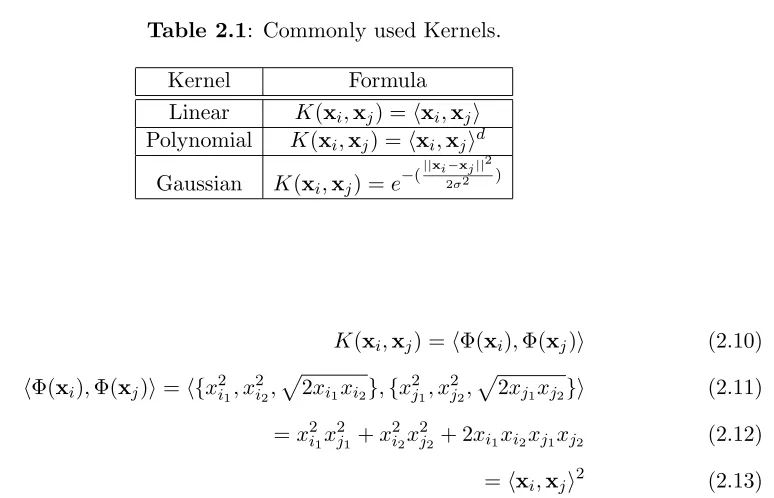
Table 2.1: Commonly used Kernels.
Kernel Formula
Linear K(xi,xj) =hxi,xji
Polynomial K(xi,xj) =hxi,xjid
Gaussian K(xi,xj) =e−(
||xi−xj||2
2σ2 )
K(xi,xj) =hΦ(xi),Φ(xj)i (2.10)
hΦ(xi),Φ(xj)i=h{x2i1, x
2
i2,
p
2xi1xi2},{x 2
j1, x
2
j2,
p
2xj1xj2}i (2.11)
=x2i1x2j1+x2i2xj22+ 2xi1xi2xj1xj2 (2.12)
=hxi,xji2 (2.13)
In this way we can compute the dot product of two instances in the transformed feature space using (2.13) meaning that we never have to explicitly evaluate the coordinates in the new feature space (as is done in (2.11)). The power of the kernel trick becomes evident when the transformation function (Φ) projects the original data into possibly infinite dimensions. A number of kernel functions that are commonly used in the literature are given in Table 2.1.
Gram Matrix
The Gram matrix (sometimes called the kernel matrix) is formed by evaluating the kernel function on the training data and storing the results in a matrix K where its element are:
Ki,j =K(xi,xj)
The dimensions of the matrix arem×mwherem is the number of documents in the training data. The Gram matrix offers an interface between the kernel component and the classifier component in a kernel machine.
Classifier Component
ˆ
f(x) =hw,xi+b (2.14)
Linear classifiers are binary therefore the predicted label is determined based on which side of the hyperplane the example lies. Figure 2.7 shows a linear classifier which separates the data. In the case of Y ={±1} the classification is simply the sign of predicted values as shown in (2.15)
h(x) =sign( ˆf(x)) (2.15)
A special characteristic of the hyperplane produced by an SVM is that the margin is maximised. The margin is the distance to the separating hyperplane from the point closest to it. It is desirable to have a large margin since it will be better able to tolerate noisy examples. In general, for a linear classifier to generalise well, a large margin should be sought. Finding the hyperplane which maximises the margin can be formulated as the following optimisation problem.
M inimise : ||w|| (2.16)
subject to : ∀(x,y)∈Dℓ :yhw·xi+b≥1 (2.17)
Lagrange multipliers are used to translate the difficultprimal optimisation problem (2.16) into an equivalent dual quadratic maximisation optimisation problem (2.18) for which there exists efficient algorithms.
M aximise : −
m
X
i=1
αi+
1 2
m
X
i,j=1
αiαjyiyjhxi·xji (2.18)
subject to :
m
X
1=1
αiyi= 0 with αi≥0 (2.19)
The result of the optimisation process is a set of coefficients α. Only those training examples which haveαi >0 contribute to the construction of the hyperplane. These examples
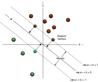
are called the support vectors and define the margin. Figure 2.7 shows a linear classifier constructed from three support vectors (highlighted) that lie on the margin.
X Y
w
Margin Support Vectors
<w,x> + b = 0
<w,x> + b = -1
[image:43.595.153.484.87.363.2]<w,x> + b = 1
Figure 2.7: SVM Classifier. The SVM is a linear classifier that constructs a hyperplane w separating the data. The hyperplane is constructed in such a way to create maximal (margin) distance between the two classes. Computational efficiency is achieved since only the three Support Vectors are required to classify further instances. In this particular example the offset parameter b is zero sincewpasses through the origin.
ˆ
f(x) =
m
X
i
αiyihxi·xi+b (2.20)
h(x) = sign( ˆf(x)) (2.21)
M aximise: −
m
X
i=1
αi+
1 2
m
X
i,j=1
αiαjyiyjK(xi,xj) (2.22)
ˆ
f(x) =
m
X
i
αiyiK(xi,x) +b (2.23)
Performance
Support vector machines have been shown to be one of the best performing classifiers for text classification (Yang & Liu, 1999; Joachims, 1997). Since the classification learning algorithm is fixed, kernel machines place the importance on choosing the correct kernel rather than choosing the correct classifier. Sometimes choosing the appropriate kernel is almost as difficult as choosing the correct classifier.
2.6.4 Ensembles
The “No Free Lunch” theorem (Wolpert, 1995) states that there is no single learning al-gorithm that always induces the most accurate classifier for every domain. Each learning algorithms will perform differently depending on the domain. Yang & Liu (1999) considers the performance of many different learning algorithms for the task of text classification. In general, for supervised learning tasks, a number of different learning algorithms will be con-sidered and the one which outputs the best performing classifier, as evaluated on a validation set, is chosen.
An alternative solution is to combine multiple classifiers together. An ensemble (or com-mittee) (Breiman, 1996) is a collection of classifiers whose individual decisions are combined in order to classify new examples. The members of the ensemble as referred to as the
base-learners. Ensembles have been shown to increase accuracy when used with reasonably
accu-rate base-learners. Ensembles perform best when the constituent base-learners are diverse. A number of methods for constructing ensembles are given below:
• Stacking. The easiest way to ensure diversity in the ensemble is to use different learning
algorithms for each base-learner.
• Parameters. Most learning algorithms are characterised by a set of user defined
• Representations. Diversity can be established by training each base-learner using a separate representation of the data. This is similar to the idea of Co-Training (Blum & Mitchell, 1998) where multiple representations of the same data exist. Similarly, one could use different kernels for each base-learner to transform the original data into different representations.
• Training Data. The most common way to construct an ensemble is to train each
base-learner with different training data. Two bootstrapping approaches have been successfully used in the literature, namely boosting and bagging.
Bagging
Bagging (Breiman, 1996) is where an ensemble of N members is constructed by sampling N
bootstrap samples from the labelled training data, with replacement. Each base-learner is induced from one of the bootstrap samples.
Boosting
Boosting, in particular AdaBoost (Schapire, 1999) is an iterative process to construct a set of complementary base-learners for an ensemble. It iteratively adds new base-learners such that the training data of base-learners added in successive iterations are tailored by the misclassifications of the base-learner in previous iterations.
A weak base-learner is induced from a subset constructed by sub-sampling from the training data according to the weights. Initially all weights are uniform but are updated based on the misclassifications of the weak base-learner. Training examples which are incorrectly classified have their weights adjusted so that they are more likely to be chosen in subsequent iterations of boosting. In this way sampling is focused on these hard to classify examples. The output of AdaBoost is an ensemble formed using all the induced weak base-learners.
Ensemble Predictions
Predictions from an ensemble are obtained by combining the predictions of the members. Ma-jority voting is the most commonly used method and simply finds the mode of the predictions in the ensemble (see (2.24)).
ˆ
f(x) = arg max
N
X
ˆ
where ˆfi is the prediction given by the ith member of the ensemble.
The use of ensembles (committees) in machine learning has grown due to the increased performance achieved. However, considerable computational overheads are encountered since numerous classifier must be induced and considered for each prediction.
2.6.5 Multi-Class Classification
We have discussed mainly binary classification problems, where there are only two possible labels for an instance and the task is to construct a function which maps input examples to one of the two possible labels. However, we often wish to solve classification problem that have more than two labels. Multi-class classification is where the number of labels is greater than two.
Certain classifiers such as the k-NN are capable of easily extending to the multi-class setting while others such as Support Vector Machines do not. To overcome this, multi-class classification problems can be decomposed into a series of binary classification problems. Two principled techniques can be employed to achieve this, namely One-v-Rest and One-v-One. Below we give some details on both techniques. For a comprehensive evaluation of various multi-class techniques please see (Hsu & Lin, 2002).
One-v-Rest
One-v-Rest (1vR) decomposes a n-class problem into nseparate binary classification prob-lems where one concept is compared with all other concepts. For example, a multi-class classification problem to identify digits would construct 10 binary classifiers, one for each digit. One such classifier would identify the digit 7 and considers all other digits to be negative examples of this concept (Vapnik, 1995).
One-v-One
2.7
PAC Learning Model
An obvious question regarding induction algorithms is how many examples are required to produce an accurate classifier. Ideally we would like the induction algorithm to construct a classifier consistent with the target function for any possible input. In other words we wish the classifier to have zero error. Unfortunately this is infeasible for two reasons.
First, to achieve zero error requires training data consisting of labelled examples for every possible input pattern. This is infeasible for all but the most trivial of problems. Second, the training data is a random sample of examples. There exists a small probability that the sample contains noisy examples that mislead the induction algorithm and result in the production of a poor classifier. Hence, the construction of a classifier consistent with the target function may not always be possible.
The Probably Approximately Correct (PAC) (Valiant, 1984; Mitchell, 1997) learning model studies the number of examples required to achieve a classifier with a bounded er-ror rate. It does so by weakening the demands on the induction algorithm. The induction algorithm is not required to succeed in constructing a classifier for every possible sequence of randomly drawn training examples. Failure is bound by some arbitrarily small parameter
δ. Furthermore, the algorithm is not required to produce a zero-error classifier. Rather it is required to produce a classifier that has error bounded by ǫ.
These bounds presented allow PAC to state that, a learner will output a classifier (hy-pothesis) with probability (1−δ) that has error less thanǫafter observing a sufficient number of training examples and after performing a reasonable amount of computation.
The number of examples required is intrinsically linked to the efficiency of the learning algorithm in the PAC learning model. Training data size is limited by the time required to process it since PAC requires the output of a hypothesis after a reasonable amount of computation.
2.8
Evaluation
A classifier induced from a set of labelled training examples will be deployed to classify new and previously unseen examples from the input space. Evaluation is concerned with estimating the performance of induced classifiers on future examples.
Induction of classifiers with zero error requires a labelled training example for every pos-sible input pattern. Since this is impractical for all but the most trivial of classification problem, induced classifiers will misclassify a certain percentage of data. The optimal perfor-mance metric to use is true error which is the probability that the classifier will misclassify a randomly drawn instance from the input space.
Error(h) =P(h(x)6=f(x))
The true error of a classifier is unknown, however, an estimate can be calculated using a number of machine learning evaluation techniques.
2.8.1 Data Partitioning
Estimates are constructed from a test set, which is a set of examples labelled by the target function and is used to evaluate the classifier performance. The test set can be constructed in a number of ways but, crucially, test data is completely unknown to the induction algorithm. In other words, test data is never used in training a classifier. Two of the most popular methods for constructing a test set are:
• Holdout Testing. This is where the training data is split into two mutually exclusive
sets. One set becomes the training data from which the classifier is induced. The second is used as the test and is used to estimate the performance of the induced classifier. Figure 2.8(a) shows this process where half of the data is used as training data while half is held back for testing data. This is called 50/50 train/test split. However, it is considered more beneficial to have a larger test set as used in the RCV1 dataset (Lewis
et al., 2004).
• k-fold-cross-validation. When the number of labelled training data is small the holdout
training data. The fold used as testing data changes in each trial. Results are averaged over all trials of the experiment. Figure 2.8(b) shows this for 4-fold cross validation.
Experiment 1
Test Data Train Data Experiment 2 Experiment 3 Experiment 4
(a) 50/50 Split
Trial 1 Trial 2 Trial 3 Trial 4
Test Data Train Data
(b) k-Fold
Figure 2.8: Data partitioning methods. The entire circle represents all the data in the corpus. (a) randomly divides the dataset into two sets, where one is used for training while the other is held back for testing. (b) shows 4-fold cross validation where in each trial one fold is held for training while all others are used for testing. The results are averaged over all trials.
The misclassifications made by the classifier on the test set are stored in a confusion
matrix from which a number of performance metrics can be calculated. In the next section
we discuss the confusion matrix next as well as a number of performance metrics commonly used in the literature. Evaluation of classifiers is an important aspect of machine learning and there are many strategies and metrics in the literature. In this review we concentrate on the most popular evaluation metrics used for text categorisation tasks.
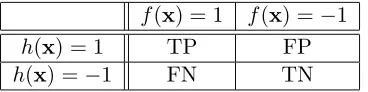
2.8.2 Confusion Matrix
Central to all of the following metrics is the confusion matrix (sometimes referred to as the contingency matrix) which encodes the errors made by a