Debt and Deficit Fluctuations in a Time Consistent Setup

Munich Personal RePEc Archive

Debt and Deficit Fluctuations in a

Time-Consistent Setup

Grechyna, Daryna

Middlesex University London

March 2015

Online at

https://mpra.ub.uni-muenchen.de/63729/

Debt and Deficit Fluctuations in a Time-Consistent

Setup

∗

,

†

Daryna Grechyna

March, 2015

Abstract

This paper compares the stochastic behavior of fiscal variables under optimal fiscal policy

for the cases of full commitment by the government (Ramsey problem) and no commitment

by the government (focusing on differentiable Markov perfect equilibrium). It shows that the

cyclical properties of fiscal variables are similar for both commitment assumptions. These

conclusions are robust to two different specifications of the structure of public bonds

(risk-free and state-contingent), and to different sets of the parameters. The cyclical properties of

fiscal variables, regardless of commitment assumptions, can be determined by the parameters

of the utility function.

Keywords: optimal taxation; time-consistent policy; market incompleteness.

JEL Classification Numbers: E61, E62, H21, H63.

∗_{This paper has been accepted to Macroeconomic Dynamics. Copyright to this article belongs to}

CAM-BRIDGE UNIVERSITY PRESS.

†_{I am very grateful to two anonymous referees and the Associate Editor, Albert Marcet, Francesc Obiols,}

Juan Carlos Conesa, Nezih Guner, my thesis committee Christopher Telmer, Hugo Rodr´ıguez, and Xavier

Mateos-Planas, the participants of the XIV Workshop on Dynamic Macroeconomics in Vigo, and the

partici-pants of the Initiative on Computational Economics 2011 in Zurich for useful comments and encouragement.

Financial support from Beca PIF of UAB is gratefully acknowledged.

‡_{Department of Economics, Middlesex University London, Business School, Hendon Campus, The}

1

Introduction

A government’s commitment to its fiscal plan is a potential determining factor of fiscal

policy outcomes. In the ideal world, the government could minimize the economic distortions

from exogenous shocks by announcing the fiscal policy once for all future periods and not

deviating from this announcement as time goes on. Practical implementation of such a

full-commitment policy is difficult; one reason for this is that this type of fiscal policy would

be time-inconsistent (see Kydland and Prescott, 1977). In modern economies, governments

usually are not fully committed to following a fiscal policy chosen in one period during future

periods. Instead, the fiscal plans are revised periodically, with the frequency of these revisions

being dependent on the institutions and on external events such as exogenous shocks or

political elections. If the economic outcomes from periodic reoptimization by the government

are significantly different from those that would occur given a government’s full commitment

to its fiscal plan, then welfare of the population may be significantly improved by constructing

mechanisms that guide the government towards full commitment.

In this paper, we analyze the effect of the absence of government commitment on the

cyclical properties of fiscal variables by comparing them to the case of full commitment.

To this end, we consider a version of the optimal fiscal policy model developed by Lucas

and Stokey (1983) with public bonds of one-period maturity and with endogenous public

spending. The government reoptimizes its fiscal plan every period, taking into consideration

the current state of the economy and the effect of current policy on the anticipated future

policy (thus, we consider the Markov perfect equilibria). The equilibrium transition path of

the analogous economy has been characterized by Debortoli and Nunes (2013) and Occhino

(2012), who showed that the optimal government policy under no commitment is such that

the time-inconsistency problem reduces over time and disappears at the steady state.

The time-inconsistency problem originates from the temptation of the government to

manipulate the price of the public bonds which are in inelastic supply. At a given period, the

discretionary government chooses to unexpectedly deflate accumulated public debt to increase

the revenue side of its budget; at the same time, it anticipates that future governments

perspective) manipulating future prices. Therefore, the current government wants to use its

discretion but it would like to force future governments to act in a committed way. The way

to do that is to decrease the time-inconsistency problem.

For a broad range of parameter values, the only stable (deterministic) steady state is

the steady state with zero public debt. The less debt, the lower the temptation to

manip-ulate prices in the future. As a result, in the long run the debt converges to a zero mean

independently of the initial level of debt. In the economy with aggregate uncertainty, where

the government mission is to mitigate the effect of exogenous shocks, the same discretion

mechanism should reduce the ability of the government to smooth taxes. Intuitively, once

debt is around zero, and because there is little temptation to manipulate prices, the

stochas-tic properties of the model should resemble those of the full-commitment case, with a lower

variance for debt and more variance in taxes, as the government tries to keep the debt around

zero to minimize the commitment problem. In this paper we verify this intuition using the

numerical simulations of the no-commitment and full-commitment economies.

We discuss two alternative structures for public bonds markets. In the first case, the

gov-ernment has access to risk-free bonds, unconditional on realization of uncertainty in the next

period. In the second case, the government has access to state-contingent bonds, conditional

on the realizations of the next period exogenous state. Marcet and Scott (2009) compare the

stochastic properties of fiscal variables under these alternative market structures when the

government is fully committed to its fiscal plan. We show that, without commitment, the

sta-tistical nature of fiscal variables changes, but the consequences for their cyclical properties are

insignificant. In particular, the public debt is stationary in the

no-commitment-incomplete-markets setup and is less persistent than output in the no-commitment-complete-no-commitment-incomplete-markets

setup, differently from the full-commitment cases with respective market structures. The

ab-sence of government commitment results in more volatile and less persistent fiscal variables,

but does not change the direction of responses of variables to exogenous shocks.

Furthermore, we show that the cyclical properties of fiscal variables, regardless of the

commitment assumption, depend on the parameters of the utility function. In particular, in

the considered setup with endogenous public expenditures and separable CRRA utility, the

elasticities of substitution of private and public consumption. An increase in productivity (a

positive supply shock) implies that both types of consumption, private and public, should

increase. One of the aims of optimal fiscal policy is to smooth taxes over time. If the public

consumption is relatively more elastic, taxes increase to finance higher government

expendi-tures, but the government deficits increase as well; opposite occurs if private consumption

is relatively more elastic. A shock to government expenditure (a demand shock) affects the

optimal public consumption directly and leads to conventional responses of fiscal variables

(a positive shock to government spending increases deficits and taxes). These findings are

related to several studies that have discussed the role of utility parameters for economic

out-comes under time-consistent optimal fiscal policy. In particular, Martin (2009) has shown

that the elasticity of consumption defines the long-run level of public debt in a model

with-out capital in which the discretionary government can issue both public bonds and money.

Barseghyan et al. (2013) have considered fluctuations of fiscal variables in a model with

political frictions; the authors successfully replicated the pattern of public debt in the U.S.,

but obtained counterfactual predictions of a counter-cyclical tax rate and pro-cyclical

pub-lic spending. We confirm the conjecture of those authors that the cycpub-licality of taxes may

depend on the curvature of utility from consumption.

For the case of full-commitment, there are numerous characterizations of the cyclical

properties of fiscal variables. For example, Chari et al. (1994) describe the stochastic

prop-erties of the business-cycle model; Aiyagari et al. (2002) characterize the stochastic behavior

of fiscal variables in the model without capital when financial markets are incomplete; Scott

(2007) studies the properties of labor taxes in the stochastic world; and Marcet and Scott

(2009) compare the cyclical properties of a variety of models under complete and incomplete

financial markets.

Several examples exist of closely related studies that have discussed the Markov perfect

equilibrium properties in line with this paper. Klein and R´ıos-Rull (2003) compare the

cycli-cal properties of optimal fiscycli-cal policy without commitment with those under full commitment

in the neoclassical growth model with a balanced government budget. In their model,

gov-ernment cannot commit to a capital income tax. The authors show that capital income

case, contrary to the full-commitment case. Klein et al. (2008) describe the Markov perfect

equilibrium for a benevolent government’s problem with a balanced budget when the

govern-ment has to choose public expenditures. Ortigueira et al. (2012) and Debortoli and Nunes

(2013) discuss optimal fiscal policy with an unbalanced budget and endogenous government

spending in a deterministic economy with and without capital, respectively. Krusell et al.

(2006) discuss a time-consistent fiscal policy with government debt and exogenous

govern-ment spending in a deterministic economy; the authors find a Markov perfect equilibrium

with discontinuous policy functions and debt time-series similar to those under full

commit-ment. Martin (in press) analyzes welfare consequences of different institutional arrangements

of time-consistent government policy.

The paper is organized as follows. Section 2 describes the model and the government

problem under different bond-market structures and with no commitment by the

govern-ment. Section 3 characterizes stability properties of the deterministic steady state under no

commitment. Section 4 compares the stochastic properties of fiscal variables under both no

commitment by the government and full commitment by the government. Sections 5 and 6

discuss the role of the utility parameters and of the bounds on debt for cyclical properties of

fiscal variables. Section 7 concludes.

2

The Model

The model represents a version of Lucas and Stokey’s (1983) economy, where a benevolent

government decides how to finance government spending through taxes on labor income

and through issues of public debt. The only departures from their original model are that

government spending is endogenous, the sources of uncertainty are a labor productivity shock

and a shock to preferences for public consumption, and bonds traded between the government

and households are only of one-period maturity.1 _{The structure of the economy is described}

in detail below.

The exogenous state of the economy is given by st = {θt, ϕt}, where θt represents a

shock to labor productivity and ϕt represents a shock to the marginal value of the public

follows a Markov process with a stationary transition matrix P; we denote byP(st+1|st) the

probability of the exogenous state beingst+1 at period t+ 1 conditional on beingstat period

t. We denote byst _{the history of the exogenous state from the initial period until t and by}

Pt(st_|s

0) the probability ofst conditional on s0, where s0 is given.

The economy is inhabited by identical households. The time endowment of a

representa-tive household is 1 for each period of time. The resource constraint of the economy satisfies:

ct(st) +gt(st) = θt(1−xt(st)), (1)

wherect(st_{), gt(s}t_),andxt(st_{) denote the periodt private consumption, public consumption,}

and leisure, respectively. At period t, a representative household derives utility from private

consumption and leisure, h(ct(st_{), xt(s}t_{)), separable in its arguments, as well as utility from}

public consumption, ϕtv(gt(st_{)). Functions h and v are twice differentiable, increasing and}

concave in their arguments. The total instantaneous utility function of the household can be

denoted as u(ct(st_{), xt(s}t_{), gt(s}t_{)) ≡ h(ct(s}t_{), xt(s}t_{)) +ϕtv(gt(s}t_{)). The household consumes}

and saves in the form of public bonds out of labor income net of tax payments and interest

income from its holdings of government bonds.

The benevolent government sets the labor taxesτt(st_{) and chooses the amount of public}

bonds to issue at time t to finance a stream of government spending and be repaid at time

t + 1, maximizing the welfare of the representative household; initial public debt is given.

It is assumed that the government cannot default on its debt; it repays all its obligations

outstanding on a particular date.

We consider two different structures for the public bonds, risk-free and state-contingent

(as in Aiyagari et al., 2002), and analyze the implications for the cyclical properties of

fiscal variables. Risk-free public bonds are unconditional on the realization of uncertainty

at period t+ 1. We refer to the case in which the government has access only to risk-free

public bonds as the case of incomplete markets and denote by bt(st_{) the amount of risk-free}

public bonds issued by the government at time t. State-contingent public bonds represent

a vector indexed to possible realizations of uncertainty at t + 1. We refer to the case in

which the government has access to state-contingent bonds as the case of complete markets

and denote by {bt(st+1_)}

government at time t. The labor taxes and public expenditures are chosen within a period

and are state-contingent. All debt issued by the government is held by the public.

Given the government policy, which is defined by the level of government expenditures and

taxes, a representative household chooses its consumption, leisure, and savings to maximize

its expected lifetime utility

∞

X

t=0

X

st

βtu(ct(st), xt(st), gt(st))Pt(st|s0), (2)

subject to its budget constraint. We denote by pt the price of a public bond in units of time

t consumption. In the case of risk-free public bonds, the household chooses the sequence

{ct(st_{), xt(s}t_{), bt(s}t_)}∞

t=0 and its budget constraint is given by:

ct(st) +pt(st)bt(st)≤(1−τt(st))θt(1−xt(st)) +bt−1(st−1). (3)

In the case of state-contingent public bonds, the household chooses the sequence {ct(st_),

xt(st_{), {bt(s}t+1_)}

st+1∈S}

∞

t=0 and its budget constraint is given by:

ct(st) +

X

st+1∈S

pt(st+1)bt(st+1)≤(1−τt(st))θt(1−xt(st)) +bt−1(st). (4)

It is assumed that the issues of public debt are such that the transversality condition of the

household’s problem is satisfied. The environment is competitive and the wage in period t is

equal to θt. The government faces a budget constraint that restricts its spending on public

consumption and public debt services from exceeding the tax revenues and income from the

newly issued bonds:2

gt(st) +bt−1(st−1)≤τt(st)θt(1−xt(st)) +pt(st)bt(st),

if bonds are risk−f ree; (5)

gt(st) +bt−1(st)≤τt(st)θt(1−xt(st)) +

X

st+1∈S

pt(st+1)bt(st+1),

if bonds are state−contingent.

A competitive equilibrium in the considered economy, given government policy and the

initial public debt, consists of stochastic processes for bond prices and a household’s allocations

the household’s expected lifetime utility subject to its budget constraint; the government budget

constraint is satisfied; and the resource constraint of the economy is satisfied.

The optimality conditions of a representative household set its intratemporal choice of

consumption and leisure as a function of income taxes,

ux,t(xt(st))/uc,t(ct(st)) = (1−τt(st))θt, (6)

and intertemporal choice of consumption levels as a function of bond price,

pt(st)uc,t(ct(st))−β X st+1∈S

P(st+1|st)uc,t+1(ct+1(st+1)) = 0,

if bonds are risk−f ree; (7)

pt(st+1)uc,t(ct(st))−βP(st+1|st)uc,t+1(ct+1(st+1)) = 0,∀st+1 ∈S,

if bonds are state−contingent.

For the case of state-contingent bonds, (7) represents a system of equations for each state

st+1. The optimality conditions (6) and (7) can be used to substitute away taxes and prices

from the household budget constraint to obtain the implementability constraint to be taken

into account by the government:3

ct(st)uc,t(ct(st)) +β X st+1∈S

P(st+1|st)uc,t+1(ct+1(st+1))bt(st) =

=ux,t(xt(st))(1−xt(st)) +uc,t(ct(st))bt−1(st−1), if bonds are risk−f ree; (8)

ct(st)uc,t(ct(st)) +β X st+1∈S

P(st+1|st)uc,t+1(ct+1(st+1))bt(st+1) =

=ux,t(xt(st))(1−xt(st)) +uc,t(ct(st))bt−1(st), if bonds are state−contingent.

The resource and implementability constraints (1) and (8) implicitly define the optimal

con-sumption and leisure of the household as functions of government policy (described next)

and the exogenous state.

2.1

Government Policy

The government is unable to commit to a fiscal plan developed for the long term. Instead,

public expenditures and labor income taxes) every period, given the inherited debt and the

stochastic state of the economy. That is, the government policy functions depend only on

fundamentals. The policy chosen by the government in a given period affects the state of the

economy (in particular, the amount of debt outstanding) in the next period, which in turn

defines the next period policy choices of the government, and so on. This effect of current

policy on the anticipated future policy is taken into account in the government maximization

problem.

The government decides on its policy before households make their choices about the

variables they control. The decisions are made only once for each period of time and after

the exogenous shocks have been realized. Under such policy-making timing, the optimal

allocations of households in a given period represent the reaction functions on the

govern-ment policy undertaken in that period; differently from the governgovern-ment, a representative

household’s choices do not have direct influence on the future government policy.

Given that policy chosen by the government depends only on the state of the economy,

we switch to a shortcut notation, useful for recursive formulation of the government problem.

First, we change the notation for the amount of risk-free bondsbt−1(st−1) tob andbt(st) tob′.

Second, we change the notation for the amount of state-contingent bonds bt−1(st) tobs and

{bt(st+1)}st+1∈S to {b

′

s′}_s′_∈S. Finally, we substitute the time subindex t+ 1 with superindex

prime and drop the time subindextand the argumentsst_orst+1_{from the remaining variables.}

Then, the resource constraint (1) reads as

c+g =θ(1−x), (9)

and implementability constraint (8) reads as:

cuc(c) +βX s′_∈S

P(s′|s)u′_c(c′)b′ =ux(x)(1−x) +uc(c)b, or

cuc(c) +β

X

s′_∈S

P(s′|s)u_c′(c′)b′_s′ =u_x(x)(1−x) +u_c(c)b_s, (10)

in the case of risk-free public bonds and state-contingent public bonds, respectively.

The problem of the current government can be formulated in terms of household

alloca-tions: the government chooses consumption, leisure, and the amount of new public bonds

amount of public bonds to be repaid in current period, the exogenous state, and the fact

that anticipated future policy depends on the government’s current policy via the amount

of public bonds to be repaid in the future. In particular, (10) includes future consumption

implemented by the next period government, depending on the inherited level of debt and

the realization of uncertainty.4

Let Γ∈[B

¯; ¯B] be the set of possible debt levels, B¯<0<B¯. In the case of risk-free public bonds (incomplete markets), the states of the economy are b and s. Denote as C(b, s) the

policy that the current government operating under incomplete markets anticipates will be

followed in the future, so that c′ _=C(b′_{, s}′_{). Then, givenb,s, and the perception that future}

governments implement C(b, s) with corresponding net present value utility V(b, s),

substi-tuting g from the resource constraint (9), the problem of the current government operating

under incomplete markets can be formulated as follows:

max

c,x,b′

(

u(c, x, θ(1−x)−c) +βX s′_∈Θ

P(s′|s)V(b′, s′)

)

, (11)

s.t. :uc(c) +βX s′_∈Θ

P(s′|s)u′_c(C(b′, s′))b′ =ux(x)(1−x) +uc(c)b. (12)

In equilibrium, the anticipated policy function will coincide with the actual policy function.

We can define the equilibrium in the case of risk-free public bonds as follows:

A Markov perfect equilibrium in a given incomplete markets economy consists of functions

V(b, s), C(b, s), X(b, s), and B(b, s) such that for all (b, s)∈Γ×S:

{C(b, s),X(b, s),B(b, s)}= argmax

c,x,b′

{u(c, x, θ(1−x)−c) +βX s′_∈Θ

P(s′|s)V(b′, s′)},

subject to (12); and

V(b, s) = u(C(b, s),X(b, s), θ(1−X(b, s))−C(b, s)) +βX s′_∈Θ

P(s′|s)V(B(b, s), s′).

In the case of state-contingent public bonds (complete markets), the states of the economy

are bs and s. Denote as C(bs, s) the policy that the current government operating under

complete markets anticipates will be followed in the future, so thatc′ _=C(b′

bs, s,and the perception that future governments implementC(bs, s) with corresponding net

present value utility V(bs, s), substituting g from the resource constraint (9), the problem of

the current government operating under complete markets can be formulated as follows:

max

c,x,{b′ s′}s′ ∈Θ

(

u(c, x, θ(1−x)−c) +βX s′_∈Θ

P(s′|s)V(b′_s′, s′)

)

, (13)

s.t.:ux(x)(1−x) +uc(c)(b−c)−βX s′_∈Θ

P(s′|s)u′_c(C(b′_s′, s′))b′_s′ = 0. (14)

A Markov perfect equilibrium in a given complete markets economy consists of functions

V(bs, s), C(bs, s), X(bs, s), and {Bs′(bs, s)}_s′_∈Θ, such that for all (bs, s)∈Γ×S:

{C(bs, s),X(bs, s),{Bs′(bs, s)}_s′_∈Θ}= argmax

c,x,{b′ s′}s′ ∈Θ

{u(c, x, θ(1−x)−c)+βX s′_∈Θ

P(s′|s)V(b′s′, s′)},

subject to (14); and

V(bs, s) =u(C(bs, s),X(bs, s), θ(1−X(bs, s))−C(bs, s)) +βX s′_∈Θ

P(s′|s)V(Bs′(bs, s), s′).

Assume that equilibrium policy functions are differentiable under both complete and

incomplete markets.5

The necessary conditions for government problems (11)-(12) or (13)-(14) consist of (9),

(10), and the following equations (see derivations in appendix):6

ux−θug−γ(uxx(1−x)−ux) = 0, (15)

and

uc−ug−γ(ucc(b−c)−uc) = 0 and (16)

βX

s′_∈Θ

P(s′|s)[γu′_c+γu′_ccC′_bb′−γ′u′_c] = 0, if bonds are risk−f ree, (17)

or

uc−ug−γ(ucc(bs−c)−uc) = 0 and (18)

γu′c+γu′ccC′bsb

′

s−γ′u′c = 0,∀s′ ∈S, if bonds are state−contingent, (19)

where γ is the Lagrange multiplier attached to the implementability constraint (10). Note

The respective government problems under full commitment are formulated in the

ap-pendix. Equations (15) and (16)-(17) or (18)-(19) are close to their full commitment

coun-terparts (equations (21)-(23) or (25)-(27) in the appendix), but do not include the term that

measures the effect on the current government budget constraint of maintaining the price of

the bond consistent with the value of the bond in the previous period (this term is described

in appendix). Instead, equations (17) and (19) include either the termγu′

ccC′bb′ orγu′ccC′bsb

′

s,

each of which measures the effect of current government budget constraints on the policy

choices of future governments (that is, the impact of choice of debt in the present on future

choices).

In equilibrium, the reaction by households to discretionary government policy should

reduce the ability of the government to smooth economic fluctuations in comparison to the

full-commitment case under both complete and incomplete bond markets. The importance

of government discretion as compared with full commitment by the government is evaluated

in the following sections using numerical simulations.

3

Deterministic Steady States

In a deterministic setup, equation (17) or (19) implies that the model economy features three

types of steady states: 1) b = 0, 2)Cb = 0 with γ 6= 0, and 3) γ = 0. In all three cases, the

time-inconsistency problem disappears.

The steady state without distortionary taxation,γ = 0,is not stable and is also

character-ized byCb = 0.7 In equilibrium with a sufficiently large amount of accumulated assets, there

is no need to rely on distortionary taxation, and allocations are unaffected by government

policy.

The stability properties are not easily characterized for the other two types of steady

states: 1) b = 0 and 2) Cb = 0 with γ 6= 0. Only for a restricted set of parameters is it

possible to prove analytically that the steady state with b = 0 is asymptotically stable (e.g.

when utility is linear in leisure). To explore the stability properties of these types of steady

For further analysis, we specify the utility function with the general form as follows:

u(ct, xt, gt) = φc c

1−vc

t

1−vc +φx x1−vx

t

1−vx + (1−φc−φx)ϕt g1−vg

t

1−vg, vc, vx, vg >0. (20)

In this section, we setϕt = 1, θt = 1, for allt. The weights in the utility functionsφc and

φx are chosen so that leisure accounts for 66% of the time endowment and the ratio of public

to private consumption is 0.36 in the first-best equilibrium (same values as in Debortoli and

Nunes, 2013). The discount factor β is set to 0.98 to approximately match the return on

public bonds. We consider different combinations of utility parameters: vc, vx, vg ∈[0.5; 2.5]3.

We reduce the system of optimality conditions (9), (10), (15), (16), (17) without

uncer-tainty to three equations by substituting away g and γ. For each combination of{vc, vx, vg},

we solve the resulting system of three equations, together with the first derivatives of these

equations with respect to b, at the steady stateCb = 0 and then at the steady state b = 0.

As a result, we obtain the values of C(b), X(b), B(b), and their derivatives with respect to

b, Cb, Xb, Bb, for a given set of parameters at a given steady state. If the solution features

|Bb| < 1, we conclude that the corresponding steady state is asymptotically stable. When

there are multiple solutions, we choose the solution that delivers maximum utility as the

relevant one.

The results of this exercise indicate that for all considered combinations of parameters,

the steady state Cb = 0 is not asymptotically stable (it is characterized by Bb = 1), while

the steady state b = 0 is asymptotically stable. The latter steady state is characterized by

Cb >0.8

As is well known from the literature (see, for example, Marcet and Scott, 2009), in a

deterministic environment with full commitment on the part of the government, the steady

state of the economy is determined by initial public indebtedness and is asymptotically

stable. Thus, the types of equilibrium steady states that exist without commitment by the

government are quite different from the corresponding steady states under a fully committed

government. In the case where initial public debt is zero, the full-commitment and the

no-commitment steady states coincide, and there is no time-inconsistency problem to deal

with.

presence or absence of government commitment, can affect the cyclical properties of the

economy even around the time-consistent steady state. The next sections describe the model

economies with uncertainty.

4

Comparison of No- and Full-Commitment Outcomes

This section compares the stochastic properties of fiscal variables under no commitment and

full commitment using simulations of the model economies. Solutions for the no-commitment

case are based on global approximations of policy functions on the grid of states. Numerical

algorithms and accuracy measures are described in the appendix. Corresponding problems

under full commitment by the government with state-contingent and risk-free bonds have

been extensively characterized in the literature (see Marcet and Scott, 2009) and are

sum-marized in the appendix.

For the purpose of simulations, the model parameters are set as follows. The weights

in the utility functions φc, φx and the discount factor β are set in the same way as in the

previous section. In the literature, vc and/or vx are usually set to one or two, while vg is

usually set to one; it can also be slightly lower or greater than one (Debortoli and Nunes,

2013). We report the results of the model simulations for vc =vx = 1, vg = {0.9,1.1}. The

role of different utility parameters is discussed in the next section.

We assume that the labor productivity shock and the public expenditure shock are

independent and follow AR(1) processes: lnθt = ρθlnθt−1 + εt, εt ∼ N(0, σ2ε), lnϕt = ρϕlnϕt−1 +ǫt, ǫt ∼ N(0, σǫ2). We set ρθ = ρϕ = 0.85 and σε = σǫ = 0.01.9 The transition

matrix for the exogenous state of the economy st = {θt, ϕt} is constructed using Tauchen’s

(1986) method.

We report the results of simulations in the form of impulse-response functions for

envi-ronments including complete and incomplete markets given either no or full commitment by

the government for the following variables: public debt, measured as the debt to be repaid

(bt), primary deficits, measured as the deficit net of debt service costs (gt −τtθt(1−xt)),

labor taxes, and output. The impulse responses are calculated as the difference between the

output in the period preceding the shock (e.g., for debt 100(bt−b0)/(θ0(1−x0)), where the

shock occurred in t = 1), excepting the labor taxes, for which the responses are calculated

as the percentage deviation from their value in the period preceding the shock.

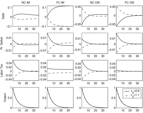
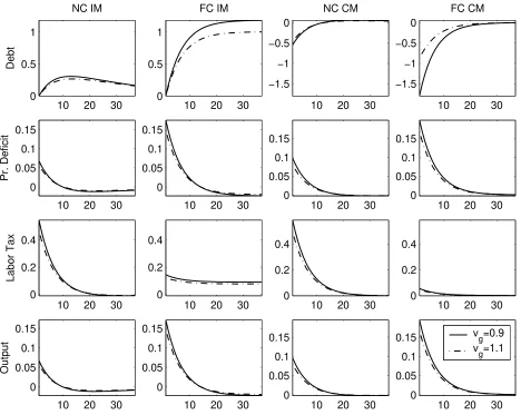
Figures 1 and 2 present the impulse responses to one standard deviation positive

produc-tivity shock and positive public expenditure shock, respectively.

[FIGURE 1]

[FIGURE 2]

We can observe the following:

i) The direction of response of fiscal variables to a shock is the same for the full-commitment

and no-commitment cases, but depends on the structure of bond markets. Moreover,

for labor productivity shock, the direction of response of fiscal variables depends on

the parameters of the utility function. In particular, given vc = vx = 1, a positive

productivity shock leads to an increase in public debt, deficits, and taxes when public

consumption is elastic, and to a decrease in these variables when public consumption

is inelastic, under incomplete markets. The direction of response of public debt is

op-posite for the complete markets case. A positive shock to government spending leads

to higher debt, deficits, and taxes under incomplete markets, for all considered utility

parameters, and to a reduction in debt under complete markets.

ii) Public debt and deficits are more volatile and taxes are less volatile under full

com-mitment, as compared to the no-commitment case, both under incomplete and under

complete markets. This reflects the role of full commitment by the government in

tax-ation smoothing. Although the time-inconsistency problem is minor around the steady

state, the magnitude of fluctuations is affected by the absence of commitment.

iii) Public debt and deficits are less persistent in the no-commitment than in the

full-commitment case (though the differences in persistency are not very significant under

complete markets). To see that, note that the responses of these variables come back to

zero faster under no commitment. Higher persistency of the variables under full

the value of previously accumulated debt, which is absent under the no-commitment

policy. In the no-commitment environment, the persistence of the variables is affected

by the impact of the state variable, public debt, on policy functions, under both bond

market structures. Previous positive indebtedness induces the government to deflate

the debt price (as also discussed in Debortoli and Nunes, 2013), reducing the reaction

of fiscal policy to the shocks.

As has been shown by Marcet and Scott (2009), under full commitment by the government

all of the variables are characterized by the same persistence as output when state-contingent

bonds are available, whereas public debt and taxes are more persistent than other variables

when only risk-free bonds are available. This is only partially true in the no-commitment

case studied here. Public debt and taxes are still the most persistent variables when the

government does not commit to fiscal policy and operates risk-free public bonds. However,

when the bonds are state-contingent, public debt is less persistent than output. Moreover,

under no commitment, the state-contingent public debt and corresponding primary deficit

inherit some characteristics of their risk-free counterparts: their response changes sign in the

long run and does not vanish over a long period of time. This persistence is because the

policy functions depend on the inherited debt in the no-commitment case under complete

markets, acting differently from the full-commitment case. Thus, regardless of the market

structure, the effect of bad shocks is partially spread over time, leading to a decrease in

deficits sufficiently far into the future to service the additional interest, similar to the

full-commitment-incomplete-markets case discussed in Marcet and Scott (2009).

Comparing these results to the four facts about the behavior of public debt and deficits

in the U.S. described in Marcet and Scott (2009), we can conclude that the first three facts

(high persistence of public debt, co-movement of deficit and debt and persistent fluctuations

in deficits) hold for the incomplete markets economy with no commitment by the government,

while the fourth fact, about pro-cyclicality of deficits and debt, is not robust to different

parametrizations of the utility function under both full and no commitment. Differences

in the directions of responses of fiscal variables for small changes in the utility parameters

impose challenges for successful calibration of the model. Therefore, this paper does not

the data.

From Figures 1 and 2 we infer that under no commitment, the government partially loses

the ability to smooth taxes in response to exogenous shocks. However, it is unclear whether

different market structures have different effects on taxation policy under no commitment

as compared with full commitment by the government. The differences in responses of

public debt are smaller when the government has access to state-contingent debt. This

is partially due to the fact that stationarity of public debt is independent of the commitment

assumption under complete markets, distinguishing it from the incomplete markets case.

With full commitment by the government when markets are incomplete, the public debt has

a unit root component that originates from an extra state variable that resembles a martingale

(see more on this in Aiyagari et al., 2002). Under no commitment, the only endogenous state

is inherited debt; therefore, the public debt is stationary regardless of the market structure.

Moreover, in the full-commitment-incomplete-markets setup, given the unit-root nature of

public debt, the bounds B

¯ and ¯B can be binding and influence the variance of public debt series (see more on the role of the bounds on debt in Section 6).

To draw an inference about the importance of market structure, we calculate the ratio

of impulse responses for labor taxes under no commitment to the corresponding impulse

responses under full commitment. The response of labor taxes is four and ten times greater

under no commitment than under full commitment with incomplete and complete markets,

respectively. The ratios of the responses of households allocations in the no-commitment and

full-commitment cases (not shown in the figures) are also greater under complete markets.

This suggests that the absence of government commitment has more severe implications under

complete than under incomplete markets. Nevertheless, similar to Aiyagari et al. (2002)

we find negligible differences in welfare across different market structures and commitment

assumptions.

Overall, the results of simulations imply that removing the government commitment

assumption changes the quantitative characteristics, but does not qualitatively affect the

cyclical properties of fiscal variables. Next, we discuss the role of different parametrizations

5

The Role of Utility Parameters

The analysis above suggests that the stability of the equilibrium under no commitment

and the direction of responses of fiscal variables to the productivity shock under both no

and full commitment by the government depend on the relative intertemporal elasticities

of substitution of the components of the utility function. To explore the latter issue, we

consider a linear approximation of the responses of variables to a productivity shock as a

function of the inverse of the elasticity of public consumption, vg, around the point vg = 1,

given vc =vx = 1. We establish the following result (see details on the numerical procedure

in appendix):

In the economy with full commitment and complete markets, given vc = vx = 1 and a

positive labor productivity shock, the response of private consumption and debt are increasing

in vg and the response of leisure, labor taxes, and deficits are decreasing in vg; moreover,

the responses of taxes, leisure, and deficit (debt) are negative (positive) for vg >1, positive

(negative) for vg <1, and zero for vg = 1.

Numerical simulations described in the previous section suggest that this result should

also hold in the economy with complete markets and no commitment (due to the similarity

of full- and no-commitment outcomes) and in the full- and no-commitment economies with

incomplete markets (for all the variables, excepting public debt, which has a response opposite

to that in complete markets). Moreover, varying the elasticity of substitution of private

consumption, given vg, has the opposite implications for the direction of responses: the

higher (lower) vc is, the more positive (negative) the response of taxes and deficits.

Sensitivity of the cyclical properties of fiscal variables to the elasticities is specific to the

economy with endogenous public spending and originates from a trade-off between public and

private consumption in a given period. Intuitively, the more inelastic public consumption

is, the more the private consumption increases in response to positive productivity shock

as compared with the public consumption. This leads to relatively greater increase in the

marginal rate of substitution between consumption and leisure and, therefore, to relatively

lower response of optimal taxes. All together, this is likely to lead to a decrease in deficits.

lead to a decrease (increase) in debt under incomplete (complete) markets.

A shock to government expenditure affects the optimal public consumption directly and

leads to conventional responses of the fiscal variables (a positive shock to government spending

increases deficits and taxes) for all combinations of parameters from the set {vc, vx, vg} ∈

[0.5; 2.5]3_{. At the same time, a positive shock to the value of endogenous government spending}

increases output, acting differently from the exogenous government spending shock that is

usually discussed in the literature. This is because an increase in the relative value of public

consumption leads to an optimal increase in the labor supply from households (the relative

value of leisure decreases).

In addition to the cyclical properties of the variables, the utility parameters affect the

response of bond price to discretionary policy: ucc depends on the elasticity of private

con-sumption. The numerical simulations suggest that the response of consumption to changes

in debt, Cb, is also sensitive to the intertemporal elasticities of substitution of private and

public consumption.

Thus, the parameters of the utility function may define the cyclical properties of fiscal

variables and the magnitude of the difference between the policies under full and no

commit-ment by the governcommit-ment.

6

The Role of Bounds on Debt, B

¯

and ¯

B

In formulating the government problem, we assumed that possible debt levels belong to set

Γ ∈ [B

¯,B¯], B¯< 0 < B¯. The bounds B¯ and ¯B are not restrictive for the no-commitment economy, which converges to the steady state with zero public debt. In equilibrium, the

households’ response to the government policy leads to a reduction in debt level until the

time-inconsistency problem disappears (in the deterministic setup) or is negligible (in the

stochastic setup). Under full commitment, the bounds on debt can be occasionally binding

and affect the volatility of variables in the incomplete markets economy (see Aiyagari et al.,

2002).

To get more insights on the role of bounds on debt, consider an alternative set of possible

debt levels: Γ ∈ [B

for the economy with no commitment by the government: a positive lower bound on public

debt fixes the distortions from discretion at the level where public debt is equal to the lower

bound.

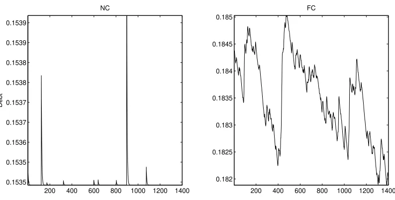
[FIGURE 3]

Figure 3 plots an example of simulations of public debt series for no-commitment and

full-commitment economies with B

¯ and ¯B equal to 50% and 70% of output (to proxy the recent OECD average debt levels). In the full-commitment case, public debt behaves as a random

walk; in the no-commitment case it converges to the lower positive bound, with occasional

insignificant deviations from the bound after the most severe shocks. Thus, restrictions that

prevent convergence of public debt to zero strengthen the differences in cyclical properties

between the full- and no-commitment environments. The further the level of public debt

is from zero, the greater the gains from the discretion are, and the greater the response

to discretion – the derivative Cb is positive and increasing in b. Given that households’

consumption function counteracts the changes in public debt for high public debt levels, it

is difficult if not impossible for the government to use public debt to smooth fluctuations

far from the steady state. In contrast, in the low level of discretion (around the steady

state), households react more to the tax-smoothing policy of the government and less to the

discretionary policy, increasing the similarity between no- and full-commitment outcomes.

7

Conclusions

This paper compared the stochastic behavior of fiscal variables under optimal fiscal policy

with no commitment by the government and full commitment by the government in an

econ-omy with endogenous government spending. It showed that the cyclicality and persistence

of the variables are not significantly affected if the government reoptimizes its policy every

period instead of committing to a fiscal plan chosen once for an infinite number of time

periods in the future. This result suggests that the timing of policymaking is not necessarily

the defining force of the model’s outcomes.

This paper also showed that the parameters of the utility function can affect the cyclical

substi-tution of private and public consumption define the direction of responses of public debt,

deficits, and taxes to a supply (the labor productivity) shock. This finding represents a

challenge for the calibration of optimal fiscal policy models.

Notes

1

Thus, the particular management of the maturity of public debt to make the full-commitment policy

time-consistent, as proposed by Lucas and Stokey (1983) and Dom´ınguez (2005), or to complete the market,

as proposed by Angeletos (2002), cannot be applied.

2

There is no need to introduce public transfers to ensure that the government budget constraint will be

always satisfied with equality. Whenever the government constraint is loose, welfare may be improved by

increasing the level of public spending; it will not distort the household’s decisions, given that public spending

enters the utility in an additive way.

3

Thus, the primal approach to solve the government problem is used.

4

In case of non-separable preferences, (10) also includes future labor; future government spending is defined

by the feasibility constraint.

5

The corresponding equilibrium for a deterministic economy has been analyzed by Debortoli and Nunes

(2013). They show that equilibrium with differentiable policy function exists for the particular utility function.

6

Here and in the appendix we skip the arguments of the functions to simplify the notation.

7

To see this, note that without distortionary taxation, the first-order conditions corresponding to the

control variables become uc = ug = ux. These equations define steady-state consumption and leisure as

functions only of the utility parameters. Thus, consumption and leisure are constant over time and are

independent of public debt. Substituting consumption and leisure into (8) without uncertainty yields, in this

steady state,B_{b= 1/β; that is, this steady state is unstable.}

8

Further numerical experiments suggest that the steady state b = 0 is not stable (|B_{b| > 1) for some}

combinations of considered parameters when the weights in the utility functions φc, φx are chosen so that

the ratio of public to private consumption is less than 0.36 in the first-best equilibrium.

9

The exact values of these parameters are not crucial given that it is not a quantitative exercise.

References

[1] Aiyagari, S. Rao, Albert Marcet, Thomas J. Sargent, and Juha Sepp¨al¨a (2002) Optimal

[2] Angeletos, George-Marios (2002) Fiscal policy with noncontingent debt and the optimal

maturity structure. The Quarterly Journal of Economics 117, 1105–1131.

[3] Barseghyan, Levon, Marco Battaglini, and Stephen Coate (2013) Fiscal policy over the

real business cycle: A positive theory. Journal of Economic Theory 148, 2223–2265.

[4] Chari, V.V., Lawrence J. Christiano, and Patrick J. Kehoe (1994) Optimal fiscal policy

in a business cycle model. Journal of Political Economy 102, 617–652.

[5] Debortoli, Davide and Ricardo Nunes (2013) Lack of commitment and the level of debt.

Journal of the European Economic Association 11, 1053–1078.

[6] Dom´ınguez, Bego˜na (2005) Reputation in a model with a limited debt structure.Review

of Economic Dynamics 8, 600–622.

[7] Judd, Kenneth L. (1992) Projection methods for solving aggregate growth models.

Jour-nal of Economic Theory 58, 410–452.

[8] Klein, Paul, Per Krusell, and Jos´e-V´ıctor R´ıos-Rull (2008) Time-consistent public policy.

Review of Economic Studies 75, 789–808.

[9] Klein, Paul and Jos´e-V´ıctor R´ıos-Rull (2003) Time-consistent optimal fiscal policy.

In-ternational Economic Review 44, 1217–1245.

[10] Krusell, Per, Martin F.M., and Jos´e-V´ıctor R´ıos-Rull (2006) Time-consistent debt.

Manuscript.

[11] Kydland, Finn E. and Edward C. Prescott (1977) Rules rather than discretion: The

inconsistency of optimal plans. Journal of Political Economy 85, 473–492.

[12] Ljungqvist, Lars and Thomas J. Sargent (2000)Recursive Macroeconomic Theory.

Cam-bridge: MIT press.

[13] Lucas Jr, Robert E. and Nancy L. Stokey (1983) Optimal fiscal and monetary policy in

[14] Marcet, Albert and Ramon Marimon (2011) Recursive contracts. Economics Working

Papers 552, Barcelona Graduate School of Economics.

[15] Marcet, Albert and Andrew Scott (2009) Debt and deficit fluctuations and the structure

of bond markets. Journal of Economic Theory 144, 473–501.

[16] Martin, Fernando M. (2009) A positive theory of government debt. Review of Economic

Dynamics 12, 608–631.

[17] Martin, Fernando M. (2013) Government policy in monetary economies. International

Economic Review 54, 185–217.

[18] Martin, Fernando M. (in press) Policy and welfare effects of within-period commitment.

Macroeconomic Dynamics.

[19] Occhino, Filippo (2012) Government debt dynamics under discretion.The B.E. Journal

of Macroeconomics 12.

[20] Ortigueira, Salvador, Joana Pereira, and Paul Pichler (2012) Markov-perfect optimal

fiscal policy: the case of unbalanced budgets. Economics Working Papers we1230,

Uni-versidad Carlos III.

[21] Scott, Andrew (2007) Optimal taxation and OECD labor taxes. Journal of Monetary

Economics 54, 925–944.

[22] Tauchen, George (1986) Finite state markov-chain approximations to univariate and

Appendix

Derivation of the optimality conditions (15), (16), (17) and (15), (18), (19)

In the case of risk-free bonds, attaching the multiplierγ to the constraint (10) the

first-order conditions to the problem (11)-(12) are as follows:

[x] : ux−θug−γ(uxx(1−x)−ux) = 0,

[c] : uc−ug+γ(uc+cucc−uccb) = 0,

[b′] : βX s′_∈S

P(s′|s) [V_b′ +γu′_ccC′_bb′+γu′_c] = 0.

Using the Envelope condition:

Vb =ucCb+uxXb+ug(−θXb−Cb) +

γ(ucCb+cuccCb−uccCbb−uc−uxx(1−x)Xb +uxXb) +

+γβX

s′_∈S

P(s′|s) [(u′_ccC′_bb′+u′_c)b′_b+βV_b′B′_b].

Combining the Envelope condition with the first-order conditions and simplifying obtains:

Vb =−γuc.

Forwarding the last equation one period and substituting back into the first-order condition

yields the optimality conditions (15), (16), (17).

In the case of state-contingent bonds, attaching the multiplier γ to the constraint (10)

the first-order conditions to the problem (13)-(14) are as follows:

[x] : ux−θug −γ(uxx(1−x)−ux) = 0,

[c] : uc−ug+γ(uc+cucc−uccbs) = 0,

[b′_s] : V_b′_s+γu′_ccC_b′_sb′_s+γu′_c = 0,∀s′ ∈S.

Combining the Envelope conditions which defineVbs for each states∈S with the first-order

conditions and simplifying obtains:

Vbs =−γuc,∀s

Forwarding the last equation one period and substituting back into the first-order condition

yields the optimality conditions (15), (18), (19).

The optimality conditions for the government problem under full commitment

Under full commitment, the government maximizes (2) subject to (1) and (8), choosing

its fiscal plan in period 0 for all the infinite periods of the economy’s life. This economy is

similar to the economy studied by Aiyagari et al. (2002), except that public spending is

endogenous.

In the case of risk-free bonds, the optimality conditions to the government’s problem

consist of (9), (10), and the following equations:

uc−ug+µuccb−γ(ucc(b−c)−uc) = 0, (21)

ux−θug−γ(uxx(1−x)−ux) = 0, (22)

βX

s′_∈S

P(s′|s)[µ′u′_c −γ′u′_c]−v1+v2 = 0, (23)

µ′ =γ, v1(B

¯−b) = 0, v2(b−B¯) = 0, (24)

where γ is the Lagrange multiplier attached to the implementability constraint (10), b0 is

given, µ0 = 0, and v1 and v2 are the Kuhn-Tucker multipliers associated with the last two

equations, which ensure that bond issues belong to set Γ. As explained in Marcet and

Marimon (2011) and Ljungqvist and Sargent (2000), the co-state µ associated with the

government implementability constraint represents the marginal cost of commitment; namely,

of the government keeping a promise to fulfill in period t the plan announced in the previous

period. The term −µuccB, which is positive for positive debt, implies that the government

must sacrifice current consumption (uc −ug is higher) to maintain the price of the bond

consistent with the value of the bond in the previous period. This term disappears in the

optimality conditions of the government problem without commitment.

In the case of state-contingent bonds, the optimality conditions corresponding to the

government problem consist of (9) and the following equations:

ux−θug−γ(uxx(1−x)−ux) = 0. (26)

b0 =

1

uc0

∞

X

j=0

X

sj

βj cjucj−uxj(1−xj)

Pj(sj|s0), (27)

where γ is the Lagrange multiplier attached to constraint (27) and b0 is given. The

se-quence of public bond issues,{bt}∞t=1, can be obtained from equation (27) forwarded t-times,

after solving the system (25)-(27). In this case, the term that measures the effect of full

commitment is given by γuccb.

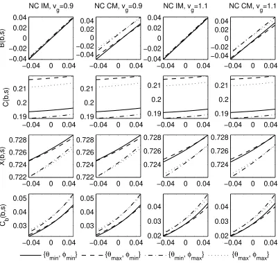
Numerical Algorithm for No Commitment

The numerical solutions for the no-commitment economies are obtained by the projection

method described in Judd (1992) using a similar procedure to that used in Martin (2013)

except that we include exogenous states as arguments rather than index the policy functions

by exogenous states. Figure 4 presents the policy functions and the derivative Cb(b, s) for

the several particular realizations of the exogenous state s.

The solutions to the government problem in the case of risk-free bonds are obtained

by solving the systems of equations (9), (10), (15), (16), (17), on a pre-specified

three-dimensional grid of states: {[B

¯; ¯B]×[1−3σ

2

θ; 1 + 3σθ2]×[1−3σϕ2; 1 + 3σϕ2]}, where σ2θ = σ2

ε

1−ρ2 θ, σ

2

ϕ =

σ2 ǫ

1−ρ2

ϕ, [B¯; ¯B] =±15% of output, and by iterating on the fixed points of the policy

functions. The policy functionsC(b, s), X(b, s),B(b, s),where s={θ, ϕ}, are approximated

by 3-cubic splines.

The solutions to the government problem in the case of state-contingent bonds are

ob-tained by solving the systems of equations (9), (10), (15), (18), (19), on the same pre-specified

grid of the states for the functions C(bs, s) and X(Bs, s), which are approximated by

3-cubic splines. The debt policy {B(bs, s′_)}

s′_∈S is conditional on the realization of uncertainty,

s′ _={θ′_{, ϕ}′_{}. Given the stationarity of the shocks, all possible realizations of the next period’s}

exogenous state, conditional on the current period state, are defined by S. Therefore, the

debt function in the complete markets case is approximated by a 5-cubic spline on the grid

{[B

¯; ¯B]×[1−3σ

2

θ; 1 + 3σθ2]2×[1−3σϕ2; 1 + 3σ2ϕ]2}. Once a new exogenous states′ ={θ′, ϕ′}

is realized, only the portion of the debt conditional on s′_{, b}′

s′ =B(bs, s′),becomes relevant as

[FIGURE 4]

For the baseline model solution the grid consists of 11 nodes for b, 5 nodes for θ, and 5

nodes forϕ. The accuracy of approximations on the grid is evaluated with rescaled to unit-free

generalized Euler equation errors (equations (17) and (19) divided by the marginal utility of

consumption). The maximum absolute unit-free generalized Euler equation errors calculated

on the grid of 1000 equally distant nodes forbwithin [B

¯; ¯B] are: 1.03e−07 and 1.29e−07 for the incomplete markets approximation and 1.33e−06 and 1.88e−06 for the complete markets

approximation, for vg = 0.9 and vg = 1.1, respectively. An alternative accuracy measure (as

in Martin, 2013), the sum of squared residuals for each necessary optimality condition of the

government problem (reduced to three equations by substituting away g and γ), delivers the

following results: 8.92e−12, 3.38e−11, 2.22e−14 and 1.30e−11, 7.34e−11, 2.21e−14

for incomplete markets, vg = 0.9 and vg = 1.1, respectively; and 5.80e−09, 3.31e−11,

1.42e−12 and 1.19e−08,7.15e−11,3.16e−12, for complete markets,vg = 0.9 andvg = 1.1,

respectively. Increasing the number of nodes leads to moderate improvements in accuracy at

the expense of much longer computational time. Increasing the bounds of endogenous state,

b, for a given number of nodes reduces accuracy far from the steady state.

Analysis of the direction of responses of fiscal variables to a labor productivity

shock

Consider the government that operates under full commitment and issues state-contingent

bonds; assume without loss of generality that ϕt = 1 andb0 = 0.

In the case whenvg = 1, the optimality conditions (25)-(27) imply thatct= θtφ2c

(1−φx)(φx+φc),

xt = φx

φx+φc, γ=

φx−φx(φx+φc)

φc(φx+φc) , bt= 0, and equation (6) implies that, over time, τt is constant

and the primary deficit is zero.

In the case whenvg 6= 1, compute the derivatives of consumption and leisure with respect

to θt, dxt/dθt and dct/dθt, from the system (25)-(26) using the Implicit function theorem

(these two equations implicitly define ct and xt as functions of θt; γ is constant over time).

These derivatives are functions of vg. Consider their linear approximation around vg = 1:10

dxt dθt(vg)≃

dxt dθt(1) +

d(dxt/dθt)

dvg

vg=1

dct

dθt(vg)≃ dct dθt(1) +

d(dct/dθt)

dvg

vg=1

(vg −1).

Using a numerical solver, we find that d(dxt/dθt)

dvg

vg=1

<0 and d(dct/dθt)

dvg

vg=1

>0. Thus, the

response of private consumption to a positive productivity shock is increasing in vg and the

response of leisure is decreasing in vg and changing sign from positive to negative at vg = 1.

Moreover, the response of consumption is greater than the response of leisure in absolute

value, which combined with (6) implies that the response of taxes to a positive productivity

shock is decreasing in vg (and changing sign from positive to negative at vg = 1). The

public debt in period t, bt =ct/φcP∞

j=t

P

sjβj(φc+φx+φc/xj)Pj(sj|st), is increasing in ct

and decreasing in xt; thus, the response of public debt to a positive productivity shock is

increasing in vg (and changing sign from negative to positive at vg = 1). Finally, we refer to

the results from Marcet and Scott (2009) to conclude that the response of the primary deficit

Figure 1: Impulse responses to 1 standard deviation positive productivity shock.

10 20 30 −0.1

0 0.1

NC IM

Debt

10 20 30 −0.01

0 0.01

Pr. Deficit

10 20 30 −0.04 −0.02 0 0.02 0.04 Labor Tax

10 20 30 0

0.5 1

Output

10 20 30 −0.1

0 0.1

FC IM

10 20 30 −0.01

0 0.01

10 20 30 −0.04

−0.02 0 0.02 0.04

10 20 30 0

0.5 1

10 20 30 −0.05

0 0.05

NC CM

10 20 30 −0.01

0 0.01

10 20 30 −0.04

−0.02 0 0.02 0.04

10 20 30 0

0.5 1

10 20 30 −0.05

0 0.05

FC CM

10 20 30 −0.01

0 0.01

10 20 30 −0.04

−0.02 0 0.02 0.04

10 20 30 0

0.5 1

v_g=0.9 v_g=1.1

The impulse responses for debt, deficits, and output are calculated as the difference between the value of

the variable in periodtand in the period preceding the shock as the percentage of output in the period

preceding the shock; the responses for labor taxes are calculated as the percentage deviation from their

value in the period preceding the shock. Columns “NC IM” and “FC IM” present the responses for no

commitment and full commitment with incomplete markets, respectively; columns “NC CM” and “FC CM”

Figure 2: Impulse responses to 1 standard deviation positive government expenditure shock.

10 20 30 0

0.5 1

NC IM

Debt

10 20 30 0

0.05 0.1 0.15

Pr. Deficit

10 20 30 0

0.2 0.4

Labor Tax

10 20 30 0

0.05 0.1 0.15

Output

10 20 30 0

0.5 1

FC IM

10 20 30 0

0.05 0.1 0.15

10 20 30 0

0.2 0.4

10 20 30 0

0.05 0.1 0.15

10 20 30 −1.5

−1 −0.5 0

NC CM

10 20 30 0

0.05 0.1 0.15

10 20 30 0

0.2 0.4

10 20 30 0

0.05 0.1 0.15

10 20 30 −1.5

−1 −0.5 0

FC CM

10 20 30 0

0.05 0.1 0.15

10 20 30 0

0.2 0.4

10 20 30 0

0.05 0.1

0.15 vg=0.9

v_g=1.1

The impulse responses for debt, deficits, and output are calculated as the difference between the value of

the variable in periodtand in the period preceding the shock as the percentage of output in the period

preceding the shock; the responses for labor taxes are calculated as the percentage deviation from their

value in the period preceding the shock. Columns “NC IM” and “FC IM” present the responses for no

commitment and full commitment with incomplete markets, respectively; columns “NC CM” and “FC CM”

Figure 3: Simulations of the public debt series when B

¯ and ¯B are equal to 50% and 70% of the steady state output.

200 400 600 800 1000 1200 1400 0.1535

0.1535 0.1536 0.1537 0.1537 0.1538 0.1538 0.1539 0.1539

NC

Debt

200 400 600 800 1000 1200 1400 0.182

0.1825 0.183 0.1835 0.184 0.1845 0.185

FC

The time-series of public debt in the case of stochastic labor productivity, B

¯ and ¯B equal to 50% and 70%

of the steady state output. Columns “NC” and “FC” present public debt series for the no-commitment and

Figure 4: The policy functions and the derivative Cb(b, s).

−0.04 0 0.04

−0.04 −0.02 0 0.02 0.04

NC IM, v

g=0.9

B(b,s)

{θ

min, φmin} {θmax, φmin} {θmin, φmax} {θmax, φmax}

−0.04 0 0.04

−0.04 −0.02 0 0.02 0.04

NC CM, v

g=0.9

−0.04 0 0.04

−0.04 −0.02 0 0.02 0.04

NC IM, v

g=1.1

−0.04 0 0.04

−0.04 −0.02 0 0.02 0.04

NC CM, v

g=1.1

−0.04 0 0.04

0.19 0.2 0.21

C(b,s)

−0.04 0 0.04

0.19 0.2 0.21

−0.04 0 0.04

0.19 0.2 0.21

−0.04 0 0.04

0.19 0.2 0.21

−0.04 0 0.04

0.722 0.724 0.726 0.728

X(b,s)

−0.04 0 0.04

0.722 0.724 0.726 0.728

−0.04 0 0.04

0.724 0.726 0.728

−0.04 0 0.04

0.724 0.726 0.728

−0.04 0 0.04

0.03 0.04 0.05

C b

(b,s)

−0.04 0 0.04

0.03 0.04 0.05

−0.04 0 0.04

0.02 0.03 0.04

−0.04 0 0.04

0.02 0.03 0.04

The policy functions for debt, B_{(b, s), consumption,}C_{(b, s), leisure,}X_{(b, s), and the derivative}C_{b(b, s) for}

s={{θmin, φmin};{θmax, φmin};{θmin, φmax};{θmax, φmax}}. Columns “NC IM,vg= 0.9” and “NC CM,

vg= 0.9” present functions for no commitment with incomplete and complete markets, respectively, for

vg= 0.9; columns “NC IM, vg= 1.1” and “NC CM,vg= 1.1” present functions for no commitment with