Inference in Differences in Differences with Few Treated Groups and Heteroskedasticity

(1)

Munich Personal RePEc Archive

Inference in Differences-in-Differences

with Few Treated Groups and

Heteroskedasticity

Ferman, Bruno and Pinto, Cristine

Sao Paulo School of Economics - FGV, Sao Paulo School of

Economics - FGV

8 December 2015

Online at

https://mpra.ub.uni-muenchen.de/81988/

(2)

Inference in Differences-in-Differences with Few Treated

Groups and Heteroskedasticity

∗

Bruno Ferman

†

Cristine Pinto

‡

Sao Paulo School of Economics - FGV

First Draft: October, 2015 This Draft: October, 2017

Please click here for the most recent version

Abstract

We show that existing inference methods used in Differences-in-Differences might not perform well with few treated groups and heteroskedastic errors. This is restrictive because variation in the number of obser-vations per group inherently leads to heteroskedasticity in the group x time aggregate model. We provide theoretical justification and empirical evidence from placebo simulations with real datasets showing that this problem may remain relevant even in datasets with a large number of observations per group. We then derive an alternative inference method that works when there are few treated groups (or even just one) and many control groups in the presence of heteroskedasticity. Combined with feasible generalized least squares estimation, our test is uniformly most powerful under normality and a consistent estimator for the variance-covariance matrix, while it can still provide a test with correct size if the serial correlation is misspecified or errors are not normally distributed.

Keywords: differences-in-differences; inference; heteroskedasticity; clustering; bootstrap; permutation tests; Behrens-Fisher problem

JEL Codes: C12; C21; C33

∗_{We would like to thank Josh Angrist, Aureo de Paula, Marcelo Fernandes, Sergio Firpo, Bernardo Guimaraes, Michael}

Leung, Lance Lochner, Ricardo Masini, Marcelo Moreira, Marcelo Medeiros, Whitney Newey, Vladimir Ponczek, Andre Portela, Vitor Possebom, Rodrigo Soares, Chris Taber, Gabriel Ulyssea and seminar participants at Boston University, MIT Econometrics lunch, Sao Paulo School of Economics - FGV, PUC-Rio, Insper, Latin American Workshop in Econometrics, EPGE-FGV, USP, 3rd conference of the IAAE, the Bristol Econometric Study Group Annual Conference, the European Meeting of the Econometric Society, and the Africa Meeting of the Econometric Society for comments and suggestions. We also thank Lucas Finamor and Deivis Angeli for excellent research assistance. Cristine Pinto gratefully acknowledges financial support from FAPESP.

(3)

1

Introduction

Differences-in-Differences (DID) is one of the most widely used identification strategies in applied economics. However, inference in DID models is complicated by the fact that errors might exhibit intra-group and serial correlations.1 _{Not taking these problems into account can lead to severe underestimation of the DID standard}

errors, as highlighted inBertrand et al.(2004). Still, there is as yet no unified approach to dealing with this problem. As stated in Angrist and Pischke (2009), “there are a number of ways to do this [deal with the serial correlation problem], not all equally effective in all situations. It seems fair to say that the question of how best to approach the serial correlation problem is currently under study, and a consensus has not yet emerged.”

With many treated and many control groups, one of the most common inference methods used in DID applications is the cluster-robust variance estimator (CRVE) at the group level, which allows for unrestricted intra-group correlation and is also heteroskedasticity robust.2 _{With a small number of groups, it might still}

be possible to obtain tests with correct size, even with unrestricted heteroskedasticity (for example,Cameron et al.(2008),Brewer et al.(2013),Canay et al.(2014),Ibragimov and M¨uller(2010),Ibragimov and M¨uller

(2016), andMacKinnon and Webb (2015a)). However, all of these inference methods do not perform well when the number of treated groups is very small. In particular, none of these methods perform well when there is only one treated group.3 _{There are alternative inference methods that are valid with very few}

treated groups, such asDonald and Lang(2007), henceforth DL,Conley and Taber(2011), henceforth CT, and cluster residual bootstrap, analyzed byCameron et al.(2008). However, all these methods rely on some sort of homoskedasticity assumption in the group x time aggregate model, which might be a very restrictive assumption in common DID applications. For example, if there is variation in the number of observations in each group x time cell, then the group x time DID aggregate model should be inherently heteroskedastic.4

As a consequence, these methods would tend to (under-) over-reject the null hypothesis when the number of observations in the treated groups is (large) small relative to the number of observations in the control groups.5

In this paper, we first formalize the idea that variation in group sizes may lead to distortions in inference methods designed to work with very few treated groups, and we show that this problem may remain relevant even when the number of observations per group is large. More specifically, we show that there are plausible structures on the errors such that the group x time aggregate model remains heteroskedastic even when the number of observations per group goes to infinity. In placebo simulations with the American Community Survey (ACS) and the Current Population Survey (CPS), we also provide evidence that this problem can be relevant in datasets commonly used in empirical applications, even when we have a very large numbers of

1_{We refer to “group” as the unit level that is treated. In typical applications it stands for states, counties, or countries.} 2_{The CRVE was developed by} _{Liang and Zeger} _{(1986), and we can think of this method as a generalization of the}

heterocedasticity-robust variance matrix due toWhite (1980). Bertrand et al. (2004) show that CRVE at the group level works well when the number of groups is large, whileWooldridge (2003) provides an overview of cluster-sample methods in linear models and shows that CRVE provides valid inference when the number of groups increases and groups sizes are fixed.

3_{MacKinnon and Webb} _{(2015b) show that CRVE t-statistics and the wild bootstrap have important size distortions in}

this case. Canay et al.(2014) inference method for DID would have poor power when the number of treated groups is very small, as they point out in remark S.2.5, whileIbragimov and M¨uller(2010) andIbragimov and M¨uller(2016) require at least two observations in each group. Finally, the method proposed inMacKinnon and Webb(2015a) can lead to important size distortions when there are very few treated groups, as they present in their paper.

4_{Even in case of individual-level data, all these methods require (implicitly or explicitly) some kind of aggregation at the}

group x time level. Therefore, this problem is relevant whether one considers DID regressions using individual-level or aggregate data.

5_{The problem of variation in group sizes leading to heteroskedasticity and, therefore, to distortions in methods that rely}

(4)

observations per group. For example, in placebo simulations with the ACS, rejection rates at 5% significance level (under the null) for tests that rely on homoskedasticity are close to zero when the number of observations in the treated group is above median, and close to 10% when it is below median. Therefore, while DL argue that a large number of observations per group would justify the homoskedasticity assumption and CT provide an extension of their method that would be valid with individual-level data when the number of observations per group grows at the same rate as the number of control groups, we provide a theoretical justification and empirical evidence based on real datasets showing that these results would not be valid under more complex (and more plausible) structures on the errors.6

We then derive an alternative method for inference when there are only few treated groups (or even just one) and errors are heteroskedastic. The main assumption is that we can model the heteroskedasticity of a linear combination of the errors.7,8 _{Under this assumption, we can re-scale this linear combination of}

the residuals of the control groups using the (estimated) heteroskedasticity structure so that they become informative about the distribution of this linear combination of the errors of the treated groups. Importantly, the main advance of our method is that, by focusing on a linear combination of the errors, we circumvent the need to impose strong assumptions and to specify a structure for the intra-group x time and serial correlations. Moreover, we also circumvent the incidental parameter problem caused by the estimation of group fixed effects with a finite number of time periods. We show that a cluster residual bootstrap with this heteroskedasticity correction provides valid hypothesis testing asymptotically when the number of control groups goes to infinity, even when there is only one treated group. Our Monte Carlo simulations and simulations with real datasets (the ACS and the CPS) suggest that our method provides reliable hypothesis testing when there are around 25 groups in total (1 treated and 24 controls). It is important to note that no heteroskedasticity-robust inference method in DID performs well with one treated group. Therefore, although our method is not robust to any form of unknown heteroskedasticity, it provides an important improvement relative to existing methods.

CT present in their online appendix an example model that would allow for temporal dependence and heteroskedasticity depending on group sizes. However, the method they propose imposes strong assumptions on the structure of the errors. For example, they assume stationarity and a separability of the errors in the group x time aggregate model into two Gaussian processes, one capturing dependence and another one heteroskedasticity. This essentially implies that the serial correlation can only come from a common shock that affects all observations in a group x time in the same way, which should not be a plausible assumption for researchers using, for example, the CPS.9_{In contrast, our method is robust to a much wider}

variety of assumptions on the structure of the errors, allowing for more complex intra-group and serial correlations without the need to parametrically specifying them, even if the correlation between individuals within a group depends on variables that are unobserved by the econometrician. While it may be possible

6_{In both cases, their methods would work when the number of observations goes to infinity}_if _{there is a common group x}

time error, but would fail when there is no common group x time error. The intuition is that, when the number of observations goes to infinity, the average of the individual-level error will beop(1), while the average of a common shock that equally affects everyone in the same group x time cell will remainOp(1). We show that there might be more complex structures on the errors in which the aggregate group x time errors areop(1), but ignoring intra-cluster correlations would still underestimate the standard errors. In such cases, the aggregate model remains heteroskedastic even when the number of observations per cell goes to infinity.

7_{The crucial assumption for our method is that, conditional on a set of covariates, the distribution of a linear combination}

of the errors does not depend on treatment status. We consider a stronger assumption that the conditional distribution of this linear combination of the errors is i.i.d. up to a variance parameter in order to reduce the dimensionality of the problem.

8_{While our method is more general, this assumption would be satisfied in the particular example in which the}

heteroskedas-ticity is generated by variation in the number of observations per group.

9_{We show in Appendix}_A.6_{that the method proposed in the online appendix of CT may lead to significant size distortions}

(5)

to apply the method suggested in CT in their online appendix under a different set of assumptions, this would require derivation of a different set of moment conditions, which is complicated by the fact that conventional estimators of the time series model’s parameters based on the DID residuals would be biased due to the problem of incidental parameters (see e.g. Hansen(2007)). In contrast, by focusing on a linear combination of the errors, our method circumvents the incidental parameter problem and, as a consequence, it is straightforward to implement.10_’11

Our inference method can also be combined with feasible generalized least squares (FGLS) estimation. The use of FGLS to improve efficiency of the DID estimator has been proposed byHausman and Kuersteiner

(2008),Hansen(2007), andBrewer et al.(2013). One important challenge for implementing a FGLS estimator in the DID setting is that sample analogs for the variance/covariance matrix parameters will be inconsistent when the number of periods is fixed. While these papers provide bias-corrected estimators for the parameters of the variance/covariance matrix, they rely on strong assumptions on the structure of the errors, including homoskedasticity.12 _Following _Wooldridge ₍₂₀₀₃_), _Hansen ₍₂₀₀₇_{) and} _{Brewer et al.} ₍₂₀₁₃_{) combine their}

FGLS estimators with cluster-robust inference. This way, their inference is robust to misspecification in either the serial correlation or the heteroskedasticity structures. However, with few treated groups the use of CRVE would not work. In this case, we show that it is possible to combine FGLS estimation with our inference method. If the FGLS estimator is asymptotically equivalent to the GLS estimator and errors are normally distributed, then we show that our test is asymptotically uniformly most powerful (UMP) when the number of control groups goes to infinity. If, however, we have misspecification of the serial correlation, the estimators of the serial correlation parameters are inconsistent, or we do not have normality, then a t-test based on the FGLS estimator would not be valid, while our test can still provide the correct size. Therefore, our method provides an important safeguard for the use of FGLS estimation in DID applications with few treated groups.

With only one treated group, we show that the assumption that we can model the heteroskedasticity of a linear combination of the errors can only be relaxed if we impose instead restrictions on the intra-group correlation. If we assume that, for each group, errors are strictly stationary and ergodic, then we show that it is possible to apply Andrews’ (2003) end-of-sample instability test on a transformation of the DID model for the case with many pre-treatment and a fixed number of post-treatment periods. This approach works even when there is only one treated and one control group. We also consider the use of linear factor models for estimation of regional policies treatment effects, as suggested by Gobillon and Magnac(2013). This approach requires both many control groups and many pre-treatment periods, but it allows selection into treatment to freely depend on unobserved heterogeneity terms. We show that CT and our inference methods can be extended to linear factor models when there are only a few treated groups.

Another estimation method for the case with few treated groups when the number of pre-treatment periods is large is the synthetic control (SC) estimator (Abadie and Gardeazabal(2003) and Abadie et al.

(2010)). Abadie et al.(2010) recommend a permutation test for inference with the SC method using as test statistic the ratio of post-/pre-treatment mean squared prediction error (MSPE). If the variance of transitory

10_{Stata do-files to implement our method are available at}_{https://sites.google.com/site/brunoferman/}_.

11_{In an earlier version of their paper (Conley and Taber} _{(2005)), CT also propose another alternative to this problem,}

where they consider a deconvolution problem to separately estimate the distributions of the common group x time error and of the individual-level error. This solution, however, would also require strong modeling assumptions on the structure of the errors. In particular, it heavily relies on an error structure that can be decomposed between a common shock that affects every observations equally in a group x time cell and an idiosyncratic shock that is independent across individuals. Moreover, this method relies on sieve estimators and, consequently, requires non-trivial bandwidth choices.

12_{Hausman and Kuersteiner}_{(2008) assume that the variance/covariance matrix is block diagonal with the same block for}

(6)

shocks is the same in the pre- and post-treatment periods, then dividing the post-treatment MSPE by the pre-treatment MSPE helps adjust the variance of the test statistic in the presence of heteroskedasticity. However, Ferman and Pinto (2017) show that this permutation test can have important size distortions under heteroskedasticity if the number of pre-treatment periods is finite. In contrast, our main inference method works even when the number of pre-intervention periods is small, and it does not rely on any kind of stationarity assumption on the time series.

Our inference method is also related to the Randomization Inference (RI) approach proposed byFisher

(1935). The RI approach assumes that the assignment mechanism is known. In this case, it would be possible calculate the exact distribution of the test statistic under the null (Lehmann and Romano(2008)). We argue that the RI approach would not provide a satisfactory solution to our problem. First, a permutation test would not provide valid inference if the assignment mechanism is unknown.13 _{Moreover, even under}

random assignment, a permutation test would only remain valid for unconditional tests (that is, before we know which groups were treated). However, unconditional tests have been recognized as inappropriate and potentially misleading conditional on a particular data at hand.14 _{In our setting, once one knows that the}

treated groups are (large) small relative to the control groups, then one should know that a permutation test that does not take this information into account would (under-) over-reject the null when the null is true. Therefore, such test would not have the correct size conditional on the data at hand.15

Finally, our paper is also related to the Behrens-Fisher problem. They considered the problem of hy-pothesis testing concerning the difference between the means of two normally distributed populations when the variances of the two populations are not assumed to be equal.16 _{In order to take intra-group and serial}

correlation into account, we consider a linear combination of the errors such that the DID estimator collapses into a simple difference between treated and control groups’ averages. Therefore, our method would work in any situation in which the estimator can be rewritten as a comparison of means. For example, this would be the case for experiments with cluster-level treatment assignment. While there are several solutions to this problem with good properties even in very small samples, there is, to the extend of our knowledge, no solution for the case where there is only one observation in one of the groups.17 _{Our assumption that,}

conditional on a set of observable variables, the distribution of the errors does not depend on treatment status guarantees that we can learn about the distribution of the treated groups based on the residuals of the control groups, while still allowing for some heteroskedasticity. We focus on the case of DID estimator because the scenario of very few treated groups and many control groups is more common in this case.

The remainder of this paper proceeds as follows. In Section 2 we present our base model. We briefly explain the necessary assumptions in the existing inference methods, and explain why heteroskedasticity usually invalidates inference methods designed to deal with the case of few treated groups. Then we derive

13_{This would be the case if, for example, larger states are more likely to switch policies.} _Rosenbaum_{(2002) proposes a}

method to estimate the assignment mechanism under selection on observables. However, with few treated groups and many control groups, it would not be possible to reliably estimate this assignment mechanism. Note that it is possible that the DID identification assumptions are valid even when the assignment mechanism is not uniform.

14_{Many authors have recognized the need to make hypothesis testing conditional on the particular data at hand, including}

Fisher(1934),Pitman(1938),Cox(1958),Cox(1980),Fraser(1968),Cox and Hinkley(1979),Bradley Efron(1978), Barndorff-Nielsen(1980),Barndorff-Nielsen(1983),Barndorff-Nielsen(1984),Hinkley(1980),Mcullagh(1984),Casella and Goutis(1995), andYates(1984)

15_{This is essentially the same issue that we document for CT method. In fact, CT propose an alternative way to implement}

their method which isheuristicallymotivated by the literature on permutation tests and randomization inference.

16_See_Behrens_(1929),_Fisher _(1939),_Scheffe_(1970), _Wang_{(1971), and}_{Lehmann and Romano}_(2008). _{Imbens and Kolesar}

(2016) show that some methods used for robust and cluster robust inference in linear regressions, such asBell and McCaffrey (2002), can be considered as natural extensions of inference procedures designed to the Behrens-Fisher problem.

17_{For example,}_{Ibragimov and M¨}_uller_{(2016) provide valid tests at conventional significance levels as long as there are at least}

(7)

an alternative inference method that corrects for heteroskedasticity even when there is only one treated group. In Section 3 we extend our inference method to FGLS estimation. In Section 4 we consider an alternative application of our method that relies on a different set of assumptions when the number of pre-treatment periods is large. In Section 5, we extend our inference method to linear factor models with few treated groups. We perform Monte Carlo simulations to examine the performance of existing inference methods and to compare that to the performance of our method with heteroskedasticity correction in Section

6, while we compare the different inference methods by simulating placebo laws in real datasets in Section

7. We conclude in Section8.

2

Base Model

2.1

A Review of Existing Methods

Consider first a group x time DID aggregate model:

Yjt=αdjt+θj+γt+ηjt (1)

whereYjtrepresents the outcome of groupj at timet;djt is the policy variable, soαis the main parameter

of interest;θj is a time-invariant fixed effect for group j, whileγtis a time fixed-effect;ηjtis a group x time

error term that might be correlated over time, but uncorrelated across groups. Depending on the application, “groups” might stand for states, counties, countries, and so on.

We start considering a group x time DID aggregate model because it is well known that this way we take into account any possible individual-level within group x time cell correlation in the errors (DL andMoulton

(1986)). Therefore, we can focus on the inference problems that are still unsettled in the literature, which is how to deal with serial correlation and heteroskedasticity when there are few treated groups. However, both the diagnosis of the inference problem with existing methods and the solutions we propose are valid whether we have aggregate or individual-level data.18

There are N1 treated groups andN0 control groups. Let us start assuming thatdjt changes to 1 for all

treated groups starting after datet∗_{. In this case, the DID estimator will be given by:}

ˆ

α = 1

N1

X

j=1

"

1

T−t∗

T

X

t=t∗₊₁

Yjt−

1

t∗

t∗ X

t=1

Yjt

#

−_N1

0

N

X

j=N1+1

"

1

T−t∗

T

X

t=t∗₊₁

Yjt−

1

t∗

t∗ X

t=1

Yjt

#

= α+ 1

N1

X

j=1

Wj−

1

N0

N

X

j=N1+1

Wj

whereWj =_T₋1_t∗

PT

t=t∗₊₁ηjt−_t1∗

Pt∗

t=1ηjt.

The variance of the DID estimator, under the assumption that ηjt are independent across j, is given

by:19

var(ˆα) =

₁

N1

2 N1

X

j=1

var(Wj) +

₁

N0

2 N

X

j=N1+1

var(Wj) (2)

18_{Note that, without individual-level covariates, the DID estimator with individual-level data will be numerically the same}

as the estimator with aggregated data if we use the number of observations per group x time cell as sampling weights.

(8)

Note that the variance of the DID estimator is the sum of two components: the variance of the treated groups’ pre/post comparison and the variance of the control groups’ pre/post comparison. We allow for any kind of correlation betweenηjtandηjt′, which is captured in the linear combination of the errorsWj.

When there are many treated and control groups,Bertrand et al.(2004) suggest that CRVE at the group level works well, as this method allows for unrestricted intra-group and serial correlation in the residualsηjt.

One important point is that this method is not only cluster-robust, but also heteroskedasticity-robust. The CRVE has a very intuitive formula in the DID framework:20

\

var(ˆα)Cluster =

1

N1

2 N1

X

j=1

c

Wj2+

1

N0

2 _XN

j=N1+1

c

Wj2 (3)

whereWcj =_T₋1_t∗

PT

t=t∗₊₁ηˆjt−_t1∗

Pt∗

t=1ηˆjt.

With CRVE, we calculate each component of the variance of the DID estimator separately. In other words, we use the residuals of the treated groups to calculate the component related to the treated groups, and the residuals of the control groups to calculate the component related to the control groups. This way, CRVE allows for unrestricted heteroskedasticity. When both the number of treated and control groups goes to infinity, the DID estimator is asymptotically normal, and we can consistently estimate its asymptotic variance using CRVE. However, equation3 makes it clear why CRVE becomes unappealing when there are few treated groups. In the extreme case whenN1= 1, from the OLS normal equations we will havecW1= 0

by construction. Therefore, the variance of the DID estimator would be severely underestimated (as noticed

inMacKinnon and Webb(2015b)). The same problem applies to other clustered standard errors corrections such as BRL (Bell and McCaffrey (2002)). It is also problematic to implement heteroskedasticity-robust cluster bootstrap methods such as pairs-bootstrap and wild cluster bootstrap when there are few treated groups. In pairs-bootstrap, there is a high probability that the bootstrap sample will not include a treated unit. Wild cluster bootstrap generates variation in the residuals of eachjby randomizing whether its residual will be ˆηjt or−ηˆjt. However, in the extreme case with only one treated, the wild cluster bootstrap would

not generate variation in the treated group, sincecW1= 0. Another alternative presented byBertrand et al. (2004) is to collapse the pre- and post-information. This approach would take care of the auto-correlation problem. However, in order to allow for heteroskedasticity, one would have to use heteroskedasticity-robust standard errors. In this case, this method would also fail when there are few treated groups.

It is clear, then, that the inference problem in DID models with few treated groups revolves around how to provide information on the errors related to the treated groups using the residuals ˆηjtof the treated groups.

Alternative methods use information on the residuals of the control groups in order to provide information on the errors of the treated groups. These methods, however, rely on restrictive assumptions regarding the error terms. DL assume that the group x time errors are normal, homoskedastic, and serially uncorrelated. Under these assumptions, the test statistic based on the group x time aggregate model will have a student-t distribution. The assumption that errors are serially uncorrelated, however, might be unappealing in DID applications (Bertrand et al.(2004)).

CT provide an interesting alternative inference method that allows for unrestricted auto-correlation in the error terms and also relaxes the normality assumption. Their method uses the residuals of the control groups to estimate the distribution of the DID estimator under the null. One of the key differences relative to DL is that CT look at a linear combination of the residuals that takes into account any form of serial

(9)

correlation instead of using the group x time level residuals. In the simpler case with only one treated group, ˆ

α−αwould converge toW1 whenN0 → ∞. In this case, they use{cWj}Nj=20+1 (a linear combination of the control group residuals) to estimate the distribution of W1. While CT relax the assumptions of no auto-correlation and normality, it requires that errors are i.i.d. across groups, so that {cWj}Nj=20+1 approximates the distribution of W1 when N0 → ∞. Finally, cluster residual bootstrap methods resample the residuals while holding the regressors constant throughout the pseudo-samples. The residuals are resampled at the group level, so that the correlation structure is preserved. It is possible that a treated group receives the residuals of a control group. Therefore, a crucial assumption is again that errors are homoskedastic.

A potential problem with these methods, as originally explained in CT, is that variation in the number of observations per group might generate heteroskedasticity in the group x time aggregate model. DL argues that a large number of observations per cell would justify the homoskedasticity assumptions, while CT consider an extension of their method to individual-level data, and they show that their method remains valid if the number of observations per group grows at the same rate as the number of number of controls. However, we show in Section2.2that these methods may not be valid even when the number of observations per group is large under plausible assumptions on the structure of the errors. In their online appendix and in an earlier version of their paper (Conley and Taber(2005)), CT also suggest alternative strategies for the case with fixed sample sizes that vary across group x time cells. We show in Section2.3that the alternative method we propose relies on weaker assumptions on the structure of the errors and is more straightforward to implement.

2.2

Leading Example: Variation in Group Sizes

In this section, we formalize the idea that the group x time DID aggregate models will be inherently het-eroskedastic when there is variation in the number of observations per group and derive the implications of this heteroskedasticity for these inference methods. Moreover, we show that the aggregate group x time model may remain heteroskedastic even when the number of observations per cell is large. It is important to point out, however, that this is not the only case that might generate heteroskedasticity in the group x time aggregate DID model, and that our inference method derived in Section2.3is more general and can be applied in other settings.

We start with a simple individual-level DID model:

Yijt =αdjt+θj+γt+νjt+ǫijt (4)

whereYijtrepresents the outcome of individualiin groupjat timet;νjtis a group x time error term (possibly

correlated over time), andǫijt is an individual-level error term. The main features that define a “group” in

this setting are that the treatment occurs at the group level and that errors (νjt+ǫijt) of two individuals in

the same group might be correlated, while errors of individuals in different groups are uncorrelated. For ease of exposition, we start assuming thatǫijtare all uncorrelated, while allowing for unrestricted auto-correlation

inνjt, and then we consider more complex structures. Importantly, our correction will require much weaker

assumptions on the error structure, as will be presented in Section2.3.

When we aggregate by group x time, our model becomes the same as the one in equation1:

(10)

If we letM(j, t) be the number of observations in group j at timet, then:

ηjt=νjt+

1

M(j, t)

M(j,t)

X

i=1

ǫijt (6)

where the errors in the group x time aggregate model (ηjt) are heteroskedastic acrossj, unless M(j, t) is

constant acrossj.21

Under the assumption that we have a panel of repeated cross-sections, so thatǫijt are not correlated over

time, and assuming for simplicity that M(j, t) =Mj is constant across t, we have that the variance of Wj

conditional onMj is given by:

var(Wj|Mj) = var

1

T −t∗

T

X

t=t∗₊₁

ηjt−

1

t∗

t∗ X

t=1

ηjt|Mj

!

=A+ B

Mj

for constantsAandB, regardless of the auto-correlation ofνjt.22

Importantly, for a much wider range of structures on the errors, the conditional variance ofWj givenMj

will still have a parametric formula given in equation7that depends on only two parameters. For example, if we had a panel and allow for the individual-level residuals to be auto-correlated, then we would have another term that would depend on the ǫijt auto-correlation parameters divided by the number of observations, so

we would still end up with the same formula,var(Wj|Mj) =A+_MB

j. This formula may also remain valid

even in situations where the correlation between two observations in the same subgroup (for example, the same municipality or the same school) is stronger than the correlation between two observations in the same group but in different subgroups (for example, observations in the same state but in different municipalities). More specifically, we can consider a model:

Yikjt=αdjt+θj+γt+νjt+ωkjt+ǫikjt (7)

for individual i in subgroup k, group j and time t, where we allow for a common subgroup shock ωkjt in

addition to the group-level shock νjt. If the number of subgroups for each groupj grows at the same rate

as the total number of observations, then this model would also generate var(Wj|Mj) =A+ _MB

j. Notice

also that we do not need to assume that the individual-level model is homoskedastic to have the formula

var(Wj|Mj) =A+_MB

j.

This heteroskedasticity in the error terms of the aggregate model implies that, when the number of observations in the treated groups are (large) small relative to the number of observations in the control groups, we would (over-) underestimate the component of the variance related to the treated group when we estimate it using information from the control groups. This implies that inference methods that do not take that into account would tend to (under-) over-reject the null hypothesis when the number of observations of the treated groups is (large) small. This will be the case whether one has access to individual-level or aggregate data.

21_{Note that, if}_M₍_{j, t}_{) =}_Mj _{is constant across}_t_{, then the information on group sizes is already incorporated in model}₁

through the group fixed effectsθj, even thoughMjdoes not enter directly in model1.

22_{In this simpler case in which}_ǫijt_{is i.i.d., then}_A₌_var 1

T−t∗

PT

t=t∗+1νjt−t1∗

Pt∗

t=1νjt

andB=_T₋1_t∗+t1∗

var(ǫijt).

When the number of observations per group is not constant over time, the formula will be: var(Wj) = A˜ + ˜

B_T₋1_t∗

2_P

T

t=t∗+1M(1j,t)+ t1∗

2Pt∗

t=1M(1j,t)

(11)

If A >0, note that this would not be a problem whenMj → ∞. In this case, var(Wj|Mj)→A for all

j when Mj → ∞. In other words, when the number of observations in each group x cell is large, then a

common shock that affects all observations in a group x time cell would dominate. In this case, if we assume that the group x time error νjt is i.i.d., then

var(Wj|Mj)

var(Wj′|Mj′) →1 when Mj, Mj′ → ∞, which implies that the

residuals of the control groups would be a good approximation for the distribution of the treated groups’ errors even when the number of observations in each group is different. This is one of the main rationales used in DL to justify the homoskedasticity assumption in the aggregate model, and this is the main reason why the extension of CT to individual-level data when the number of observations per cell is large is valid (proposition 4 in CT).

However, an interesting case occurs whenA= 0. In this case, even thoughvar(Wj|Mj)→0 for alljwhen

Mj → ∞, the ratios

var(Wj|Mj)

var(Wj′|Mj′) remain constant even if allMj grows at the same rate, which implies that

the aggregate model remains heteroskedastic even asymptotically. Therefore, CT, DL, and cluster residual bootstrap would still tend to (under-) over-reject the null hypothesis when the number of observations of the treated groups are (large) small relative to the number of observations of the control groups even when there is a large number of individual observations. Note that we might have A ≈0 under complex (and plausible) conditions on the structure of the errors in which standard inference using OLS regression on the individual-level data would be unreliable. For example, we would haveA ≈0 in model 4 ifǫijt is serially

correlated and var(νjt)≈0. This may be the case if we have a panel of individual observations, as in the

CPS. Alternatively, in model7we might have that most of the intra-group correlation comes from individuals in the same subgroup (that is, var(ωkjt)>0 while var(νjt)≈0), which would also imply that A≈0. In

both cases, var(Wj|Mj)→0 whenMj → ∞, but the aggregate model remains heteroskedastic even when

Mj is large.23 In Section 7, we present results from placebo simulations with real datasets and provide

evidence that this problem is relevant in large datasets commonly used in empirical applications. Taken together, these results suggest that one should be careful when applying methods such as those proposed in CT and DL even when there is a large number of observations in all group x time cells.

2.3

Inference with Heteroskedasticity Correction

We derive an inference method that uses information from the control groups to estimate the variance of the treated groups while still allowing for heteroskedasticity. Intuitively, our approach assumes that we know how the heteroskedasticity is generated, which is the case when, for example, heteroskedasticity is generated by variation in the number of observations per group. Under this assumption, we can re-scale the residuals of the control groups using the (estimated) structure of the heteroskedasticity in a way that allows us to use this information to estimate the distribution of the error for the treated groups. Importantly, our method only requires information on the heteroskedasticity structure for a linear combination of the errors, which implies that we do not have to impose strong assumptions on the structure of the serial correlation of the errors. While we motivate our method based on heteroskedasticity generated by variation in the number observations in each group, it is important to note that our method is more general, and we can consider any observable variable that may generate heteroskedasticity in the model, such as the standard textbook case in which the conditional variance is an exponential function of a subset of covariates.

More formally, we assume we have a total ofN groups where the first j = 1, ..., N1 groups are treated.

23_{CRVE at the individual level (in the first example) and at the subgroup level (in the second example) should work well}

(12)

For simplicity, we consider first the case wheredjt changes to 1 for all treated groups starting after known

date t∗_{. Let}_X

j be a vector of observable covariates that do not necessarily enter in model1 anddj be an

indicator variable equal to 1 if group j is treated.24 _{We will define our assumptions directly on the linear}

combination of the errorsWj =_T₋1_t∗

PT

t=t∗+1ηjt−_t1∗

Pt∗

t=1ηjt. The main assumptions for our method are:

1. {Wj, Xj}is i.i.d. acrossj∈ {1, ..., N1}, i.i.d. acrossj∈ {N1+ 1, ..., N}and independently distributed across j∈ {1, ..., N}.

2. Wj|Xj, dj d

=Wj|X˜j, where ˜Xj is a subset of Xj.

3. Wj|X˜j has the same distribution across ˜Xj up to a scale parameter.

4. E[Wj|Xj, dj] =E[Wj|Xj] = 0.

5. The conditional distribution ofWj givenXj is continuous.

Note that assumption 1 allows the distribution of{Wj, Xj}for the treated groups to be different from the

distribution for the control groups. Therefore, we might consider a case where treated states have different characteristics Xj (including population sizes) than states in the control group.25 Assumption 2 implies

that, conditional on a subset of observable covariates, the distribution ofWj will be the same independently

of the treatment status. This is crucial for our method, as it guarantees that we can extrapolate information from the control groups’ residuals to estimate the distribution of the treated groups’ errors. This assumption would not be required with large N1 and N0 for inference with heteroskedasticity-robust methods. In this case, the DID would be asymptotically normal and it would be possible to allow for different distributions conditional on treatment status since there would be enough observations to estimate the variance component related to the treated groups using only information from the treated groups. In our setting, this would not be feasible since we assume that the number of treated groups is fixed and small. Assumption 3 implies that the distribution ofWj|Xj only depends onXj through the variance parameter.26 This assumption reduces

the dimensionality of the problem. It might be possible to relax this assumption and estimate the conditional distribution ofWj|X˜j non-parametrically. However, this would require very large number of control groups.

Without assumption 3, we can still guarantee that we can recover a distribution with the correct expected value and variance for the DID estimator. This should provide significant improvement relative to existing inference methods.27 _{Finally, condition 4 is the standard identification assumption for DID.}

Our method is an extension of the cluster residual bootstrap with H0 imposed where we correct the residuals for heteroskedasticity. In cluster residual bootstrap with H0 imposed, we estimate the DID re-gression imposing that α = 0, generating the residuals {cWR

j }Ni=1. If the errors are homoskedastic, then, under the null,cWR

j converges in distribution toWj whenN0→ ∞, which would have the same distribution across j. Therefore, we could resample with replacement B times from {cWR

j } N

i=1, generating {cWj,bR} N i=1,

24_{Note that we allow for covariates that vary with time, as we may consider the observations for each time period}_t_{as one}

component in vectorXj.

25_{Note that assuming}_{_{Wj, Xj, dj}_}_{is i.i.d. would also allow for the distribution of} _{_{Wj, Xj}_}_{conditional on}_dj_{= 1 to be}

different from the distribution of{Wj, Xj}conditional ondj= 0. However, we do not state assumption 1 this way because we want to consider the asymptotic whenN1is fixed andN0→ ∞.

26_{As noticed in}_{Ibragimov and M¨}_uller_{(2016) and}_{Canay et al.}_{(2014), if both the number of pre- and post-treatment periods}

are large and we can apply a central limit theorem to 1

t∗

Pt∗

t=1ηjt and T−1t∗

PT

t=t∗+1ηjt, then Wj will be approximately

normal. In this case, assumption 3 would be guaranteed.

27_{For example, in our setting, CT method would recover a distribution with different variance relative to the distribution of}

(13)

and then calculate our bootstrap estimates as ˆαb = _N11

PN1

j=1Wc

R j,b−

1

N0

PN

j=N1+1cW R

j,b. Importantly, note

that, in our setting, we do not need to work with the group x time residuals ˆηjt to construct our bootstrap

estimates. Instead, we can work with a linear combination of the residuals that takes into account any form of auto-correlation in the residuals.

As explained in Section2.1, the problem with cluster residual bootstrap is that it requires the residuals to be homoskedastic. In Theorem2in AppendixA.1, we show that, if we know the variance of Wj conditional

onXj, then we can re-scale the residualWcj,bR so that it has (asymptotically) the same distribution asWj.

First, we normalize each observedcWR j′ byWc

norm j′ =cW

R j′

1

√_var

(Wj′|Xj′). Then we generate a bootstrap sample

with the re-scaled residuals Wfj,b =Wcj,bnorm

p

var(Wj|Xj). As a result, this procedure generates bootstrap

estimators ˆαb = _N1₁PN 1

j=1Wfj,b−_N1₀P_jN₌_N1+1Wfj,b that can be used to draw inferences about αwith the correct size.28 _{The main assumption we need is that} _{_W

j}Nj=1, which is a linear combination of the error

terms ηjt, are independent across j and have the same distribution up to the variance parameter. It is

important to note that we only need to know the variance of a linear combination of the errors. This point is crucial for our method, because we do not need to specify the serial correlation structure of the errors

ηjt. The main problem, however, is that var(Wj|Xj) is generally unknown, so it needs to be estimated.

In Theorem3in Appendix A.1, we show that this heteroskedasticity correction works asymptotically when

N0 → ∞if we have a consistent estimator for var(Wj|Xj). That is, we can use var\(Wj|Xj) to generate

f c

Wj,b = cWj,bR

r

\

var(Wj|Xj)

\

var(Wj,b|Xj,b)

. Since we only need a consistent estimator for var(Wj|Xj), in theory, one

could estimate the conditional variance function non-parametrically. In practice, however, a non-parametric estimator would likely require a large number of control groups.

In our leading example where heteroskedasticity is generated by variation in group sizes, we show in Section 2.2 that we can derive a parsimonious function for the conditional variance without having to impose a strong structure on the error terms. More specifically, in this example, the conditional variance function would be given by var(Wj|Xj, dj) = var(Wj|Mj) = A+ _MB

j, for constants A and B, where Xj

is the set of observable variables including Mj. We show in Lemma 4 in Appendix A.1 that we can get

a consistent estimator for var(Wj|Mj) by regressing (WcjR)2 on M1j and a constant.

29 _{Note that we do}

not need individual-level data to apply this method, provided that we have information on the number of observations that were used to calculate the group x time averages. While we present our method for the group x time aggregate model, we show below that it is straightforward to extend our method to the case with individual-level data.

Finally, a problem with cluster bootstrap methods when there are few clusters is that there will be few possible combinations of bootstrap samples (Cameron et al.(2008),Webb(2014), andMacKinnon and Webb

(2015a)). As an optional step to ameliorate this problem, we apply the idea of wild cluster bootstrap to our method. Therefore, for each j, we sample either fcWj,b with probability 0.5 or −Wfcj,b with probability 0.5.

This procedure provides a smoother bootstrap distribution. MacKinnon and Webb (2015a) recommend a

28_{As we assume a setting in which the number of treated groups is fixed and small, we consider for inference the distribution}

of ˆαconditional on{Xj}N

j=1. Note that CT would be valid as unconditional inference if we assume that {Wj, Xj}is i.i.d.

acrossj∈ {1, ..., N}. However, CT would not provide a reasonable solution conditional on the data at hand. As we show in our example in Section2.2, CT would provide a biased test conditional on the information about group sizes. If{Wj, Xj}N

i=1is not

identically distributed (as is allowed in assumption 1), then it would be unfeasible to consistently estimate the distribution of

Wjgivendj= 1 for an unconditional test, because we would only have a finite number of treated observations (unless we have more information about the distribution ofXj|dj). Therefore, it would not be possible to conduct unconditional inference.

29_When _the _number _of _observations _per _group _is _not _constant _over _time, _we _regress ₍_c_WR

j)2 on

1

T−t∗

2_P_T

t=t∗+1M(1j,t)+

1

t∗

2Pt∗

t=1M(1j,t)

(14)

similar procedure for permutation tests.

Summarizing, our bootstrap procedure, for this specific case, consists of:

1. Calculate the DID estimate:

ˆ

α= 1

N1

X

j=1

"

1

T−t∗

T

X

t=t∗₊₁

Yjt−

1

t∗

t∗ X

t=1

Yjt

#

−_N1

0

N

X

j=N1+1

"

1

T−t∗

T

X

t=t∗₊₁

Yjt−

1

t∗

t∗ X

t=1

Yjt

#

2. Estimate the DID model withH0 imposed (Yjt=α0djt+θj+γt+ηjt), and obtain{cWjR}Ni=1. Usually the null will beα0= 0.

3. Estimate var(Wj|Mj) by regressing

c

WR

j

2

on a constant and _M1_j.

4. Usevar\(Wj|Mj) to obtain the normalized residualsWcjnorm′ =Wc

R j′

1

q

\

var(W_j′|Mj′)

5. DoBiterations of this step. On thebth_iteration:

(a) Resample with replacement N times from {Wcnorm

j }Ni=1 to obtain

f c

Wj,b

N

i=1

, where fcWj,b =

c

Wnorm

j,b

q

\

var(Wj|Mj) with probability 0.5 and−Wcj,bnorm

q

\

var(Wj|Mj) with probability 0.5.

(b) Calculate ˆαb= _N11

PN1

j=1Wfcj,b−_N10

PN

j=N1+1

f c

Wj,b.

6. RejectH0at levelaif and only if ˆα <αˆb[a/2] or ˆα >αˆb[1−a/2], where ˆαb[q] denotes theqthquantile

of ˆα1, ...,αˆB.

The method described above works when all the treated groups start treatment in the same period t∗_.

Consider a general case where there are N0 control groups and Nk treated groups that start treatment

after period t∗

k, with k = 1, ..., K. We show in Appendix A.2 that, for large N0, the DID estimator is

asymptotically equivalent to a weighted average of K DID estimators, each one using one set of k >0 as treated groups and k = 0 as control groups. The weights are given by _PNk(T−t∗k)t∗k

K

k=1Nk(T−t∗k)t∗k

. Therefore, the weights increase with the number of treated groups that start treatment aftert∗

k (Nk) and are higher when

t∗

k divides the total number of periods in half. Let cW R,k

j = T−1t∗ k

PT

t=t∗

k+1ηˆ

R jt−t1∗

k

Pt∗

k

t=1ηˆjtR. We generalize

our method to this case by estimatingK functions var(\Wk

j|Mj) by regressing (Wc R,k j )

2 _{on a constant and}

1

Mj. Each function

\

var(Wk

j|Mj) provides the proper rescale for the residuals of the DID regression using k

as the treated groups. We then calculate ˆαb as a weighted average of theseK DID estimators.

We also show in AppendixA.3that our method applies to DID models with both individual- and group-level covariates. With covariates at the group x time group-level, we estimate the OLS DID regressions in steps 1 and 2 of the bootstrap procedure with covariates. The other steps remain the same. If we have individual-level data, then we run the individual-individual-level OLS regression with covariates in step 2 and then aggregate the residuals of this regression at the group x time level. The other steps in the bootstrap procedure remain the same. Finally, we extend our method to the case of individual-level data with sampling weights in Appendix

A.4.

(15)

appendix and in an earlier version of their paper (Conley and Taber(2005)) alternative methods for the case in which the number of observations per cell is finite and varies across j. However, these methods rely on stronger modeling assumptions on the structure of the errors. The method presented in the online appendix of CT assumes stationarity and a separability of the errors in the group x time aggregate model into two Gaussian processes, one capturing dependence and another one heteroskedasticity. This essentially excludes the possibility of serial correlation in the individual-level error, which should be relevant in panel datasets. By imposing a constant serial correlation parameter across groups, this method would underestimate the serial correlation of the error for smaller groups and overestimate the serial correlation of the error for larger groups. This would lead to over-rejection when the treated group is small and under-rejection when the treated group is large. In Appendix Section A.6, we show that this distortion is significant when we consider placebo simulations with the CPS. While it may be possible to apply the method suggested in CT in their online appendix under a different set of assumptions, this would require derivation of a different set of moment conditions, which may prevent applied researchers from using their method. Conley and Taber (2005) consider a deconvolution problem to separately estimate the distributions of (νj1, ..., νjT)

and (ǫij1, ..., ǫijT). Importantly, they require an additive structure of the error in a common shock that

affects all observations in a group x time and an individual-level shock, which should not be plausible in real applications. In contrast to these two alternative methods, our method is valid under a wider range of assumptions on the structure of the errors. In particular, we do not need to assume stationarity, we can allow for more complex within group correlations even if the researcher does not have information on the variables that determine whether two observations have correlated errors, and we can allow for serial correlation in the individual-level error.30

3

Improving Efficiency with a FGLS

One important feature of our inference method is that we do not need to specify the structure of the serial correlation. Moreover, since the linear combination Wj does not depend on θj, we circumvent the

incidental parameter problem caused by the estimation of group fixed effects that complicates estimation of serial correlation parameters. We consider now the use of FGLS-DID estimator to improve efficiency. This strategy, however, presents some challenges. First, one needs to impose some structure on the entire variance/covariance matrix. Also, the residual ˆηjt depends on the group fixed effects estimator, which will

not be consistent if T is fixed. This complicates the estimation of the variance/covariance matrix even if parametric assumptions on the variance/covariance matrix are correct, as argued inHansen(2007). Finally, with few treated groups, the FGLS estimator might not be normally distributed even whenN0 → ∞. We show now that it is possible to combine FGLS estimation with our inference method. This will allow for robust inference in case the serial correlation is misspecified, estimators for the serial correlations parameters are biased, or errors are not normally distributed.

Since we assume that errors are uncorrelated across j, the variance/covariance matrix of ηjt is block

diagonal withT×T blocks given by Ωj. We assume that Ωj= Ω( ˜Xj). LetΩ( ˜b Xj) be an estimator of Ω( ˜Xj)

that converges to ¯Ω( ˜Xj) (we allow ¯Ω( ˜Xj)6= Ω( ˜Xj), so Ω( ˜b Xj) is inconsistent). The FGLS estimator using

30_{While it may be possible to apply the method suggested in CT in their online appendix under a different set of assumptions,}

(16)

b

Ω( ˜Xj) will be a linear estimator ˆαFGLS =

PT

t=1

PN

j=1ˆajtYjt. In Appendix A.5, we show that, in the case

with only one treated group, ˆαFGLS d

→PTt=1¯a1tη1twhenN0→ ∞, where ¯a1= (¯a11, ...,a¯1T)′ is defined by:

¯

a1 = argmin

a1

a′1Ω( ˜¯ X1)a1 (8)

subject to:

T

X

t=t∗+1

a1t= 1 and T

X

t=1

a1t= 0

Therefore, defining the linear combination W∗ j =

PT

t=1¯a1tηjt, we show in AppendixA.5that all results

from Section2.3apply to the FGLS estimator. The only difference is that the assumptions should be based on the linear combinationW∗

j instead of on the linear combinationWj. Note thatWcj∗R d

→W∗

j whenN0→ ∞, so there would not be an incidental parameter problem by looking at the linear combinationWj∗.31 For our

leading example presented in Section2.2, we would still havevar(W∗

j|Mj) =A+_MB

j for constantsAandB.

So far, we only assumed thatΩ( ˜b Xj) converges to ¯Ω( ˜Xj) whenN0→ ∞. So our inference method is valid even if ¯Ω( ˜Xj)6= Ω( ˜Xj). Ifηjt is multivariate normal and ¯Ω( ˜Xj) = Ω( ˜Xj), then we show in Appendix A.5

that our test has asymptotically the same power as a t-test based on the infeasible GLS estimator, which is the uniformly most powerful (UMP) test in this case.32 _{By combining our method with FGLS estimation}

we provide a test that is asymptotically UMP if all these assumptions are satisfied. Importantly, if the serial correlation is misspecified, the estimators of the serial correlation parameters are inconsistent, or the error is not normally distributed, then our test would still have the correct size while a t-test based on the FGLS estimator would be biased. Therefore, our inference method provides an important safeguard for FGLS estimation in DID settings where there are few treated groups.33 _{More specifically, we provide an alternative}

to cluster-robust inference in FGLS when it is not possible to estimate the CRVE.

4

Heteroskedasticity Correction with Large

t

∗

One of the main features of our inference method presented in Section 2.3 is that we collapse the time series structure when we consider the linear combination of the errors Wj, so that the inference problem

becomes equivalent to a comparison of means between treated and control groups. This is why our inference method does not require any specification of the time series structure. However, in the case with only one treated group, this implies that we would have, in practice, only one observation for the treated group to estimate the distribution of the treated group error. This is why a crucial assumption of our method is that

Wj|Xj, dj

d

=Wj|X˜j. Under this assumption, the residuals of the control groups are informative about the

distribution of the treated group errors. We can only relax this assumption if we impose some structure on the intra-group correlation.

We now show that, under strict stationarity and ergodicity of the time series, we can apply Andrews’ (2003) end-of-sample instability test to a transformation of the DID model if we have a large number of pre-treatment periods and a small number of post-pre-treatment periods. The main idea is that with larget∗ _and

31_{Another difference relative to the OLS DID is that we have to estimate ¯}_ajt_{. However, since we have a consistent estimator}

for ¯ajt, this does not impose any problem to apply our method.

32_{The main intuition of the proof is that, even under the alternative hypothesis, we have that}_c_W∗R j

d

→W_j∗ for alljin the control group whenN0→ ∞butN1 is small and fixed. Since the probability of resampling a treated group goes to zero, then

the bootstrap distribution will approximate the distribution of ˆαF GLS under the null even when the null is false.

33_{If we impose assumptions on the structure of the errors, then we could derive moment conditions based on}

(17)

smallT−t∗_{the DID estimator would converge in distribution to a linear combination of the post-treatment}

errors. Therefore, under strict stationarity and ergodicity, we can use blocks of the pre-treatment periods to estimate the distribution of ˆα. This is essentially the idea of the method suggested in CT, but exploiting the time instead of the cross-section variation.

If we collapse the cross-section variation using the transformation ˜Yt=_N1₁PN 1

j=1Yjt−_N1₀PN_j₌_N1+1Yjt, then:

˜

Yt=

  

˜

θ+ ˜ηt, fort= 1, ..., t∗

α+ ˜θ+ ˜ηt, fort=t∗+ 1, ..., T

(9)

where ˜θ=_N11

PN1

j=1θj−_N10

PN

j=N1+1θtand ˜ηt= 1

N1

PN1

j=1ηjt−_N10

PN

j=N1+1ηjt.

Therefore, this is a particular case of Andrews’ (2003) end-of-sample instability test in a model that includes only a constant.34 _{We want to test whether the average of ˜}_Y

tis different after the treatment. With

group-level covariates, we can estimate the OLS DID model and then construct ˜Yt usingYjt−Xjt′ βˆ. Since

ˆ

β is consistent, this approach will work under strict stationarity and ergodicity ofηjt. The same approach

works if we have individual-level covariates.35

This approach might be interesting because we do not need to assume the structure of the heteroskedas-ticity. Also, this approach works even if we have as few as one treated and one control group. However, this approach is unfeasible if there are few pre-treatment periods. Moreover, the stationarity assumption might be violated if, for example, there is variation in the number of observations per group across time. For example, if we divide the US states in the CPS by quartiles of number of observations for each year from 1979 to 2014, then 35 out of the 51 states belonged to 3 or 4 different quartiles depending on the survey year. In this scenario, our method using the function var(Wj|{\M(j, t)}Tt=1) would still provide a valid al-ternative, provided that we have a large number of control groups and we know how the heteroskedasticity was generated.

5

Linear Factor Model - Large

t

∗

and Large

N

₀

We now show that the inference methods we propose can be expanded to linear factor models with few treated groups. This method has been studied in the panel data setting in Bai (2009) and analyzed in detail for estimating treatment effects of regional policies as a generalization of DID inGobillon and Magnac

(2013).

Gobillon and Magnac(2013) consider a model in which the potential outcome in the absence of treatment is given by:

Yjt(0) =xjtβ+ft′λj+ηjtLF M (10)

34_{Note that the DID estimator would be given by ˆ}_α₌ 1

T−t∗

PT

t=t∗+1Yt˜ −t∗1

Pt∗

t=1Yt˜.

35_{With group-level covariates, we consider a model}_Yjt₌_αdjt₊_X′

jtβ+θj+γt+ηjt. With individual-level covariates, we

consider a modelYijt=αdjt+X_ijt′ β+θj+γt+νjt+ǫijt. In this case, we have to impose the strict stationarity and ergodicity assumptions onηjt=νjt+ 1

M(j,t)

PM(j,t)

(18)

wherexjt are covariates,λj is aL×1 vector of individual effects orfactor loadings, andftis aL×1 vector

of time effects orfactors. The treatment effect is given byαjt, so that:

Yjt(1) =Yjt(0) +αjt (11)

This model allows for more flexibility relative to the usual DID model. As shown inGobillon and Magnac

(2013), we can go back to the usual DID model by setting the restrictions λi = (θi,1)′ and ft = (1, γt)′.

They assume that we know the number of factors in the true DGP and that the factors are sufficiently strong so that the consistency condition for factors and factor loadings is satisfied.

As suggested in Gobillon and Magnac(2013), it is possible to estimate this model in two steps. In the first step, we estimate the linear factor model in equation 10 using the sample composed of non-treated observations over the whole period and treated observations in the pre-treatment (t≤t∗_{). If}_t∗_and_N

0tend

to∞, then we get consistent estimators forβ,ftandλt. In the second step, we estimate the counterfactual

term imputing the estimated β, ft and λt. More specifically, we have that the average treatment on the

treated effect in periodtis given by:

αt≡E[Yjt(1)−Yjt(0)| treated ] =E[αjt|treated ] =E[Yjt−xjtβ−λ′ift|treated ] (12)

Therefore, we can use the empirical counterpart ˆαt=_N1₁PN 1 j=1

h

Yjt−xjtβˆ−λˆ′ifˆt

i

to estimateE[αjt|treated ].

If we letN0andt∗ go to∞whileN1is fixed, then:

ˆ

αt =

1

N1

X

j=1

h

Yjt−xjtβˆ−λˆ′ifˆt

i _d

→ 1

N1

X

j=1

[Yjt−xjtβ−λ′ift] =

= E[αjt|treated ] +

1

N1

X

j=1

ηLF M

jt (13)

If we want to estimate the average treatment on the treated as defined inGobillon and Magnac(2013), we just need to use ˆα=_T₋1_t∗

PT

t=t∗₊₁αˆt. AsN0andt∗go to∞whileN1andT−t∗are fixed, ˆα−E[αjt|treated]

will converge to _T₋1_t∗

PT

t=t∗₊₁ h

1

N1

PN1

j=1η

LF M jt

i

. In other words, with fixedN1and fixed T−t∗, the error of the linear factor model estimator will be dominated by the error of the treated groups.

This result is a natural extension of CT.36 _{The key point is that common factors and factor loads}

are consistently estimated, so we can use the residuals from the linear factor model ˆηLF P

jt to estimate the

distribution ofηLF M

jt . This works because ast∗andN0tend to∞, ˆη LF P jt

d

→ηLF P

jt . Since we have botht∗→

∞andN0→ ∞, we have two alternatives in this case. We can exploit the cross-section variation using the estimated residuals from the control groups, _T₋1_t∗

PT

t=t∗₊₁ηˆ

LF M

jt forj > N1, to approximate the distribution

of the errors of the treated groups, 1

T−t∗

PT

t=t∗+1η

LF M

jt forj ≤N1. Under homoskedasticity acrossj, this

is essentially the method presented in CT applied to linear factor models with few treated groups. If errors are heteroskedastic, then we can use our method, provided that we know how the heteroskedasticity was generated. Alternatively, we can exploit the time series variation as shown in Section4provided thatηLF M

jt

is strictly stationary and ergodic.

36_{Note that we get an equivalent formula in the DID model if we let}_N

(19)

6

Monte Carlo Evidence

In this section, we provide Monte Carlo evidence of different hypothesis testing methods in DID. We assume that the underlying data generating process (DGP) is given by:

Yijt=νjt+ǫijt (14)

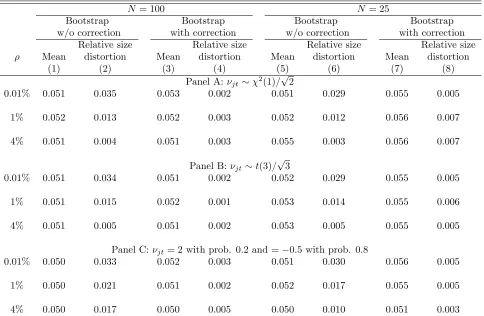
In our simulations, we estimate a DID model given by equation4where onlyj= 1 is treated andT = 2, and then we test the null hypothesis of α= 0 using different hypothesis testing methods. We focus on the case withj= 1 as this is the case in which no method that allows for unrestricted heteroskedasticity provides reliable inference. We consider variations in the DGP along three dimensions:

1. The number of groups: N0+ 1∈ {25,100}.

2. The intra-group correlation: νjt and ǫijt are drawn from normal random variables. We hold constant

the total variancevar(νjt+ǫijt) = 1, while changingρ= σ2

ν

σ2

ν+σ

2

ǫ ∈ {.01%,1%,4%}.

3. The number of observations within group: we draw, for each group j, Mj from a discrete uniform

random variable with range [M , M]∈ {[50,200],[200,800],[50,950]}.37

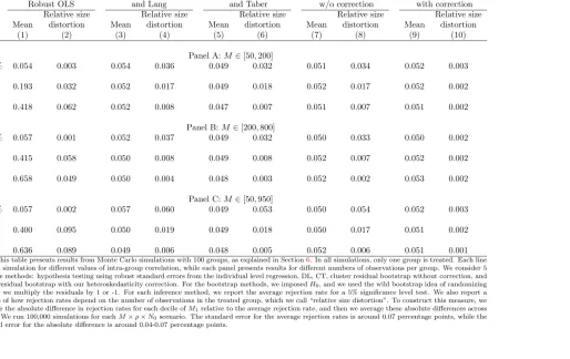
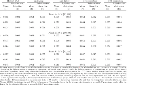
For each case, we simulated 100,000 estimates. We present rejection rate results for inference using robust standard errors in the individual-level OLS regression, and for the cluster residual bootstrap with and without our heteroskedasticity correction. All Results using DL and CT methods are similar to the results using cluster residual bootstrap without heteroskedasticity correction, as presented in the Appendix Tables. We do not include in the simulations methods that allow for unrestricted heteroskedasticity. As explained in Section2.1, these methods do not work well when there is only one treated group. We also do not include the method suggested byMacKinnon and Webb(2015a) in the simulations because their method collapses to CT when there is only one treated group. We present in AppendixA.6simulations based on the method proposed by CT in their online appendix. In both MC simulations and in simulations with the CPS, we show that their method leads to significant size distortions whenT >2 and there is serial correlation in the individual-level error.

6.1

Test Size

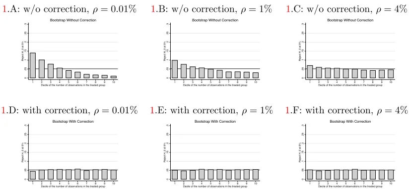
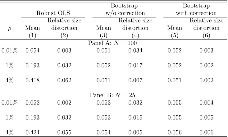
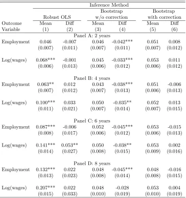
We present in Panel A of Table1results from simulations using 100 groups (one treated and 99 controls) for different values of the intra-group correlations. Column 1 shows that average rejection rates for a test with 5% significance using robust standard errors in the individual-level DID regression. The rejection rate is slightly higher than 5% when the intra-group correlationρ= 0.01% (5.4%), but increases sharply for larger values of the intra-group correlation. The rejection rate is 19% whenρ= 1% and 42% when ρ= 4%. With cluster residual bootstrap without correction, the average rejection rate is always around 5% (column 3 of Table 1). However, this average rejection rate hides an important variation with respect to the number of observations in the treated group (M1).

In Figure 1.A, we show rejection rates for cluster residual bootstrap without correction conditional on the size of the treated group for the case withρ= 0.01%. The rejection rate is around 14% when the treated

37_{In the Monte Carlo simulations, we always consider the case}_M₍_{j, t}_{) =} _Mj_{. In each simulations,} _{_Mj_}N

j=1 is redrawn

(20)

group is in the first decile of number of observations per group, while it is only 0.8% when the treated group is in the 10th decile. Note also that this distortion in rejection rates is not confined to the extremes of the distribution of group sizes. For example, the rejection rate is 3% when the treated group is in the 6th decile of number of observations per group. We summarize this variation in rejection rates by looking at the absolute difference in rejection rates for each decile ofM1 relative to the average rejection rate. Then we average these absolute differences across deciles. We call this measure “relative size distortion”. We present these results in column 4 of Table 1 for the bootstrap without heteroskedasticity correction. Conditional on the number of observations of the treated group, these methods present a relative size distortion in the rejection rates of 3.4 percentage points for a 5% significance test when ρ= 0.01%. We present rejection rates by decile of the treated group for cluster residual bootstrap without correction whenρ= 1% and when

ρ = 4% in Figures 1.B and 1.C, respectively. As expected, this variation in rejection rates becomes less relevant when the intra-group correlation becomes stronger. This happens because the aggregation from individual to group x time averages induces less heteroskedasticity in the residuals when a larger share of the residual is correlated within group. Still, even whenρ= 4% the difference in rejection rates by number of observations in the treated group remains rele