Munich Personal RePEc Archive
Updated Expectations and College
Application Portfolios
Bond, Timothy N. and Bulman, George and Li, Xiaoxiao
and Smith, Jonathan
Purdue University, University of California, Santa Cruz, The College
Board
2 February 2016
Updated Expectations and College Application Portfolios
∗Timothy N. Bond
Purdue University
George Bulman
University of California, Santa Cruz
Xiaoxiao Li
Purdue University
Jonathan Smith
The College Board
February 2, 2016
Abstract
Economists have a limited understanding of how sensitive human capital investment is to information about aptitude or likelihood of success. We shed light on this by estimating if students update their college choices in response to large positive and negative information shocks generated by the release of SAT scores. Using new data on when students select colleges to receive their scores, we find that positive shocks cause students to choose more selective colleges that charge higher tuition and have higher graduation rates. Updating is significant for students from high and low income households and for minority and non-minority students.
∗Contact information: Timothy N. Bond, [email protected]; George Bulman, [email protected]; Xiaoxiao
1
Introduction
A growing literature examines how students update their beliefs about their own aptitude during college and how this affects dropout decisions and choice of major (e.g. Zafar, 2011; Arcidiacono, Hotz, and Kang, 2012; Stange, 2012; Stinebrickner and Stinebrickner, 2012 and 2013; Wiswall and Zafar, 2015; and Arcidiacono et al. 2015). This paper provides a direct analogue at another crucial time for human capital investment – when students decide where to apply to college. Understanding how students’ beliefs about their own aptitude and likelihood of success affects their college choices is important in light of evidence that there are significant returns to college quality.1
We examine if students update their college portfolios in response to large positive and negative information shocks generated by the SAT – one of the most important components of a student’s college application.2
If students do not significantly update in response to new information about academic aptitude, it suggests that college portfolios are essentially predetermined by pre-existing beliefs and socio-economic factors.
The primary challenge to estimating student responses to information about aptitude and performance is the need to observe a panel of both college choices and the information available to students at a given point in time. A student reveals only one college portfolio and, in many cases, receives only one college entrance exam score. To overcome this, we exploit a unique policy and new data that allow us to observe the same students choosing colleges of interest before and after learning their scores. Specifically, the College Board allows students to identify a limited number of colleges to receive their scores for free at the time that they register for the exam.3
Subsequently, students learn their score on the exam and choose if and where to send additional reports. Using a new data set that indicates the exact date when each college was selected by the student, we are able to estimate the effect of SAT information shocks on the college application process.4
Conditional on sending more score reports, an unanticipated positive (negative) shock in SAT score causes a student to select a portfolio of colleges that has higher (lower) selectivity, tuition, graduation rates, and fraction of private colleges. However, the estimated effects are modest relative to cross-sectional estimates, indicating that factors such as household resources and expectations result in significant inertia in college choice.
Several factors make this environment a nearly ideal context for identifying updating of college choices. First, selecting colleges to receive SAT score reports is a high stakes decision
1
See, for example, Behrman, Rosenzweig, and Taubman (1996), Black and Smith (2006), Hoekstra (2009), and Cohodes and Goodman (2014).
2
As noted in Stinebrickner and Stinebrickner (2012), changes that “arise as students learn about their academic ability” are a “prominent alternative” to the financial explanations that dominate the literature on college enrollment decisions.
3See Pallais (2015) for analysis revealing that students tend to use each of their four free score reports. We
observe that more than three-quarters of SAT takers use at least one of their free reports, and about two-thirds of these students use all four.
4
that can impact a student’s college outcome. Second, the data include students’ Preliminary SAT (PSAT) scores and, in many cases, multiple SAT attempts. This allows us to estimate how new information from the first or second SAT score changes portfolio choice relative to old information such as the PSAT score (i.e. do students re-weight their decisions away from old information and toward new information). Third, many students appear to experience very large positive and negative realizations of scores that are difficult to predict: the standard deviation of within-student differences between first and second SAT scores is 70.3 points. Fourth, students make their pre-exam college choices shortly before taking the SAT, limiting the potential that the results are caused by time-varying factors that are correlated with exam performance.5
Finally, the analysis is based on administrative population data that produces precise estimates and allows us to consider heterogeneous effects across important socio-economic characteristics such as income and race.
We develop an empirical model based on those in the employer learning literature to motivate the empirical design.6
The model allows for information that is observable only to the student and not the researcher and for application strategies that are correlated with aptitude. The model reveals several testable implications that form the basis for the implementation and interpretation of the reduced form empirical analysis. Specifically, the model predicts updating toward the SAT and away from the PSAT for one-time takers and toward each SAT as it is revealed for those who take the exam multiple times. The model also reveals a natural test of, and correction for, students anticipating their scores.7
Identification is based on a difference-in-difference style design that estimates the extent to which college portfolios selected before and after students learn their scores reflect this new information. We find that a student who scores 100 points higher on the SAT is likely to apply to colleges whose matriculates scored about 7 points higher on the exam. This indicates that a 1 standard deviation change in a student’s score results in an approximately 0.12 standard deviation shift in the selectivity of their portfolio.8
To put this in perspective, cross-sectional estimates suggest that 100 points on the SAT is correlated with an approximately 20 point increase in portfolio selectivity after conditioning on a rich set of covariates. Thus inertia in beliefs and unobserved differences across students and households (such as parental knowledge and expectations) result in new information closing about one-third of the portfolio gap evident in the cross-section. There
5A natural concern is that changes in portfolio composition and exam performance over time are caused by a
concurrent time-varying factor such as performance in school. However, students select their pre-exam portfolios shortly before taking the SAT, not a year earlier when they take the PSAT. Thus, the pre-exam portfolio should reflect time-varying factors that are correlated with SAT performance.
6
The model is most closely related to those in Farber and Gibbons (1996), Altonji and Pierret (2001), and Lange (2007). The updating that occurs as students learn their aptitude shares similarities to the updating by employers as they observe the performance of employees (Arcidiacono, Bayer, and Hizmo, 2010; Rockoff et al., 2012; Kahn and Lange 2014). Student beliefs and updating play a significant role in theoretical models of college choice (Manski, 1989; Altonji, 1993; Altonji, Blom, and Meghir, 2012).
7Specifically, it is possible to measure the extent to which students appear to incorporate their future, unrealized
SAT score into current portfolio choices. This would occur if, for example, students could predict their scores using factors that are unobserved in the data.
8
is a similar pattern of effects for a wide range of college characteristics. For example, a 100 point higher score increases the average annual tuition of selected colleges by 400 dollars, corresponding to 6 percent of average in-state public tuition, or 0.14 standard deviations.
Among students who take the exam two times, the selectivity and composition of colleges selected after learning the score for the first exam more closely reflect that score and likewise for colleges selected after learning the second score, while the importance of the PSAT score deteriorates with each revealed SAT score.9
Importantly, the results reveal that students do not incorporate information from the second score when only the first score has been released, providing strong evidence that students do not anticipate future scores (i.e. that score variation is truly a shock). The results hold when allowing students to adopt application strategies that may be correlated with aptitude, such as applying more or less conservatively after the exam. While students generally apply more conservatively after receiving their scores, those who receive positive shocks appear to incorporate new information more than those who receive negative shocks. Further, changes in the portfolio appear to be driven by students applying more aggressively to “reach” colleges with little change in the least selective “safety” colleges. Interestingly, updating is relatively similar in magnitude for students from high and low income households, for males and females, and for students of different races.
On the extensive margin, there is little evidence that students are more likely to add colleges to their portfolios in response to score shocks. Specifically, students who experience a score shock with a magnitude of 100 points are less than one percentage point more likely to send reports to additional colleges. This suggests that students who update their beliefs the most are not over or under represented in the analysis. In contrast, the number of colleges in students’ portfolios is significantly correlated with household income and college readiness as measured by high school grade point average. Thus, the estimates should be interpreted with the awareness that higher income and better performing students are over-represented.
Higher scores on the SAT are likely to indicate an increased probability of admission and greater potential for success in college. Thus sensitivity to feedback in this context is consistent with findings in the literature that students who earn poor grades in college are more likely to drop out and that those who perform well gravitate toward more challenging majors. Altering portfolio choice in response to aptitude could partially reflect beliefs about expected returns from attending more and less selective colleges. The literature has frequently found that students alter human capital investment in response to perceived returns (Attanasio and Kaufmann, 2009; Jensen, 2010; Abramitzky and Lavy, 2014) and expectations (Jacob and Linkow, 2011). The results in this paper are consistent with the finding in Papay, Murnane, and Willett (2014) that the labels assigned to No Child Left Behind test scores affect subsequent college outcomes and that parental perceptions of child aptitude affect human capital investment (Dizon-Ross, 2014).10
The finding that revealed
9
To abstract from selection into taking the SAT one or two times, the identification design is replicated using a merged sample of one and two-time takers. The resulting estimates closely mirror those found when considering the two groups separately.
10
academic aptitude matters but plays an incomplete role in shaping college choice is consistent with results in the literature that college choices are sensitive to non-academic factors such as the availability of college counseling services (Avery and Kane 2004; Carrell and Sacerdote, 2012), information about the cost of college (Bettinger et al., 2012; Hoxby and Turner, 2014), and ease of access to entrance exams (Klasik, 2013; Hurwitz et al., 2014; Goodman, 2014; Bulman, 2015), as well as evidence of mismatch between students and colleges (Hoxby and Avery, 2012; Smith, Pender, and Howell, 2013; Dillon and Smith, 2016).
The paper is organized as follows. Section 2 describes the policy and new administrative data used to conduct the analysis. Section 3 introduces an empirical framework of student updating and identifies several testable implications. Section 4 presents the primary specifications and results. Section 5 discusses the implications of the findings.
2
SAT Scores and College Score Reports
This paper examines if students update their college portfolios in response to new information about their college-readiness and the strength of their applications. The importance of learning about aptitude for college choice depends on two factors: the weight that students place on the new information, such as SAT scores; and the magnitude of the information shock in terms of how much it deviates from prior expectations. Panel data provides an opportunity to factor out unobserved, time-invariant individual and household characteristics and beliefs that influence college choices.11
There are, however, two fundamental challenges for employing a panel data approach in this and related contexts. First, many outcomes of interest are one-time decisions that are not observed repeatedly. For example, in the typical progression, students only choose one college application portfolio, which is not conducive to observing changes over time. Second, a panel data approach requires new information that is not anticipated by students and is observed by the researcher. While students may receive large positive and negative shocks when they learn their SAT score, this is of little use if the researcher cannot account for students’ prior expectations.
This paper exploits a unique policy and a rich new dataset from the College Board to estimate the effect of information shocks generated by SAT scores on college choices. A student has only one revealed college application portfolio, but they often construct this portfolio by selecting colleges at different times. We exploit administrative data that reveal the exact timing of when students send score reports to colleges. Further, the College Board’s pricing policy induces students to select some schools to receive their SAT score before they learn their results. Our panel data thus consists
students despite reducing the likelihood of admission. 11
of information periods: the portfolio selected before learning one’s score, and the portfolio selected after learning one’s score. Further, nearly half of students take the exam a second time. This generates a third information period in which students may adapt to new information on aptitude. Multi-time takers also provide a natural test of the extent to which students anticipate scores, as we can measure the time-varying response to future score that have not been revealed yet.
2.1 SAT Data
The analysis is based on the population of SAT takers who graduated from high school between 2007 and 2009.12
The SAT is a college entrance exam administered by the College Board and is taken by high school students across the country, typically in their junior or senior years, if not both. The exam is comprised of math and critical reading sections scored between 200 and 800, so students can receive a combined score between 400 and 1600.13
Each section was normalized to have a mean score of 500 and a standard deviation of 110 in 1995. Along with student scores on each SAT attempt, the data contain Preliminary SAT/ National Merit Scholarship Qualifying Test (PSAT) scores, which is a test similar to the SAT but taken in one’s sophomore or junior year of high school. The College Board also administers a questionnaire upon exam registration that includes information on high school GPA, race, parental income, high school attended, and home zip code.
2.2 College Score Sends
Our analysis relies on observing student Score Sends, which are official SAT score reports that students have sent to colleges for consideration in the application process. The reports measure student interest in colleges and previous studies have argued that they are a reasonable proxy for applications (Card and Krueger, 2005; Pallais, 2015). Score Sends are especially advantageous for measuring updating in this setting as they reveal the intended application portfolios before and after the SAT even if the actual applications are only sent after all information has been revealed.14
The score report data include two pieces of important information. First, it reveals the college to which the report is directed. Each report sent to a four-year college is merged with college characteristics from the National Center for Education Statistics Integrated Postsecondary Education Data System (NCES IPEDS).15
Second, the data include the exact date that students request each report. When registering for the SAT, students have the option to send their scores to four colleges for no additional cost. Importantly, this must be done within nine days of taking the
12The choice of cohorts is determined by two constraints: the availability of data revealing when score reports are
sent; and the transition to a system in which students could choose which scores were sent to colleges. 13
A writing section was introduced in 2005 but not all students take this section and not all colleges use it in the admissions process.
14
For example, a student who chooses to send her score to an elite college prior to taking the SAT may not apply after receiving a lower than expected score. This is precisely the updating of beliefs that the paper is designed to estimate but would be obscured if only the final application portfolios were observed.
15Some colleges, typically two-year colleges or specialty colleges (e.g. religious or arts) do not report all of the
exam, so a high fraction of takers send reports prior to the exam. After the ten day period (or for additional reports prior to the ten day expiration), scores may be sent for a fee of approximately 11 dollars each.16
During the period of analysis, reports sent to colleges contained every score earned by the student.17
Colleges do not automatically receive a new report if a student retakes the exam. Thus reports may be sent multiple times to the same college, which is particularly common among students who improve their scores.
For students who took the SAT once, score reports are divided into those requested before taking the exam and those requested after the scores are released.18
We calculate the average characteristics of the colleges in each of these two periods, including the SAT scores of matriculating students, in-state tuition, graduation rate, and fraction private. Thus reports may be selected during three periods for students who took the exam twice: those selected prior to the first exam; those selected after the first score is released but before the second exam is taken, including reports that are free with the second registration; and those selected after the second exam scores are released. We calculate the average characteristics of the colleges in each of the three periods.
2.3 Analytic Sample
The sample for analysis includes all students in the U.S. who took the PSAT and SAT and who sent at least one score report prior to taking the SAT. The PSAT is taken by more than 75 percent of SAT takers and provides students with one measure of how they may perform. Approximately 75 percent of students send at least one free score report to a college and nearly two-thirds of score-senders use all four of their free score reports. These reports allow us to observe the types of colleges a student is considering prior to receiving new information. Analysis of revised portfolio composition is conditional on students sending score reports after taking the SAT. We explicitly estimate the determinants of sending additional reports and discuss the implications for interpreting the estimates.
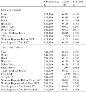
Table 1 presents summary statistics for demographic characteristics and test scores in the sample. Over 627,000 students took the SAT once and 534,000 took it twice. Approximately 46 percent are males and 59 percent are white. Mean PSAT scores are about 100, which is approxi-mately equivalent to a 1000 on the SAT. Students who took the SAT once have an average score of 1009, while students who took it twice earned a 1038 on their first attempt and a 1064 on the second attempt, on average. Approximately 21 percent of one-time takers sent scores after the exam and 32 percent of two-time takers did so after the second exam.
16
Note that students from low income households are eligible to use additional free Score Sends.
17Score Choice was adopted in the spring of 2009, whereby students could choose which SAT scores to send if there
were multiple administrations. A small number of students in the 2009 cohort may have used Score Choice, but most students do not take the SAT after the fall of their senior year (the fall of 2008).
18
2.4 Within-Student Variation in Scores
There is significant within-student variation in scores earned on the PSAT and the first and second taking of the SAT. This variation is important for two reasons. First, unpredictable variation in scores generates the information shocks necessary for identification of updating. We explicitly test for the extent to which students anticipate scores in Section 4. Second, the magnitude of the variation determines the importance of updating in practice.
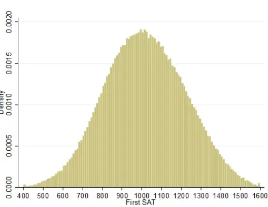
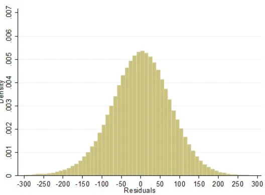
The top graph in Figure 2 presents the distribution of the differences between each students’ first SAT score and their PSAT score (after the PSAT has been multiplied by 10 to be on the same scale). While the mean is close to 0, the standard deviation of the difference is 85.6 points. That is, a student who earns a 1000 on the PSAT has an approximately 30 percent chance of earning a score lower than a 900 or greater than 1100 on the SAT. To examine the extent to which factors other than the PSAT may help to explain this variation, we generate a predicted SAT score using a rich set of observables in addition to the PSAT, including pre-exam portfolio selectivity, high school GPA, and demographic characteristics.19
The bottom graph in Figure 2 presents the difference between each student’s actual and predicted SAT score. The standard deviation of the difference is 80.5 points. That is, the rich set of observable academic and socioeconomic characteristics has essentially no additional explanatory power for predicting the SAT beyond the PSAT. This suggests that: a) the PSAT score is the most important predictor of a student’s SAT score for the researcher and perhaps the student as well; and b) there is significant within-student variation in exam scores. Within-student variation in scores is also evident in multiple takings of the SAT. The top graph in Figure 3 presents the distribution of the differences between students’ second SAT score and their first score among those who take the exam twice. The standard deviation of the difference is 70.3 points. This variation is especially interesting considering that the exams are, by design, equally difficult and cover the same body of knowledge. The time gap between when students take the exam the first and second time is frequently quite small. Note that while students perform slightly better on average the second time they take the exam (the mean of the difference is 26 points), this increase is small relative to the variation in scores. Nearly 40 percent of students earn a lower score when they take the exam again. This is notable as repeat takers have months of additional time for test preparation, experience taking the exam, and may have chosen to retake in part because they believe that they had a bad draw the first time. This suggests that there is significant noise in performance. Each student’s second score is predicted using the same list of observables as above in addition to the first SAT score. The resulting differences are presented in the bottom graph in Figure 3. The standard deviation of the difference is 63.6 points. That is, even with two measures of prior SAT scores in hand, the PSAT and the first SAT, student performance is difficult to predict.
19
This description suggests that one’s SAT score is difficult to anticipate, as students are approximately equally likely to score above or below their previous scores and the magnitude of the variation is large. Further, it is very difficult to predict the direction of the variation even with a rich set of ability and socio-economic characteristics. This descriptive analysis of score shocks is supplemented with explicit estimates of test score anticipation in Section 4. That analysis exploits the realization that if students anticipate their scores then future scores will be incorporated into current portfolio choice. There is little evidence that this is the case, suggesting that the score shocks observed by the researcher are highly correlated with the true score shocks experienced by the student.
2.5 Cross-Sectional Differences
Table 2 presents the cross-sectional relationship of portfolio selectivity with academic and non-academic factors. The resulting coefficients provide baseline context for the causal estimates pre-sented in Section 4. We regress college portfolio selectivity (as measured by the average SAT score of matriculating students) on a student’s PSAT score, SAT score, and observable characteristics including race, household income, high school attended. For one time takers, a 100 point difference in SAT score is correlated with a 20 point difference in selectivity. Thus a one standard deviation in exam score is correlated with an approximately 0.4 standard deviation difference in portfolio selectivity. Among two-time takers, each 100 points on the second SAT is correlated with an 18 point difference in portfolio selectivity. High school grade point average and socio-economic factors are also strongly correlated with the college students select. A one point change in grade point average, the difference between an A and B high school student, corresponds to a change of 30 to 50 points in portfolio selectivity, which is equivalent to about 200 points on the SAT. After controlling for student scores and grades, the difference in portfolio selectivity for households with income between 50,000 and 100,000 relative to those with more than 100,000 dollars is about 7 points.
3
Empirical Framework
take the SAT one time and two times are modeled separately, we realize that this is a choice and replicate the empirical estimates with a joint sample.
An individual forms beliefs about her optimal college application portfolio which can be summarized by a single continuous measure of quality y.20
The optimal portfolio is a function of ability that can be divided into four components: sis a set of ability correlates which are observable to both the student and the researcher (e.g. PSAT scores); q is a set of ability correlates which are observable to the student, but not the researcher (e.g. personal essays); z is the true SAT score that a student would receive in the absence of measurement error; and η is a set of ability correlates that are unobservable to both the student and the researcher (e.g. confidential letters of recommendation). The student will observe signals of z throughout the application process, the timing and content of which are known ex ante to the researcher.21
Our main interest is in testing the student’s response to these signals. Without loss of generality, we impose that η is uncorrelated with z.22
The distribution of (s, q, z, η) is assumed to be jointly normal with non-negative correlations across vectors. This assumption has been made previously in the learning literature (e.g., Lange, 2007), makes the model tractable, and there are several opportunities in the empirical analysis to examine if it is reasonable. Following the employer learning literature, the optimal portfolio for studentiis assumed to be linear in each of these elements,
yi=δqi+rsi+ Λzi+ηi (1)
where the right-hand side is the student’s true ability and is normalized to be in units of optimal portfolio choice as it has no natural scale. Hereafter we drop the subscriptiwhen it will not cause confusion.
3.1 One-Time Takers
Students who take the SAT only one time face two time periodstin which to select colleges. When t= 0, students send applications without knowledge of their SAT score. Whent= 1, students send applications having received their SAT score, z1. Beginning in t= 0, students form expectations
on their unobservable factorsz and η using their observable factors sand q. It follows from joint
20We abstract from the method by which a student determines the optimal portfolio and only assume that there
is a monotonic relationship between the quality of a portfolio and student characteristics. For theoretical treatments of the portfolio choice problem see, for example, Epple, Romano, and Sieg (2006), Chade, Lewis, and Smith (2011), and Fu (2014).
21
The model differentiates between atrue SAT score and the score a student actually receives as this allows the full set of SAT scores to matter for the application decision for individuals who take the SAT multiple times. For students who take the exam only once, imposing that there is no measurement error and that the received score is equal toz would have no consequences for the results.
22
normality that these expectations will be
z = E[z|s, q] +ν=γ1q+γ2s+ν
η = E[η|s, q] +e=α1q+α2s+e
where e and ν are mean zero normal random variables with variances σ2
e and σ
2
ν, and E[se] =
E[sν] = E[qν] = 0. The student then uses these beliefs to select an optimal period 0 application portfolio,
y0 = Ω0E[y|s, q] (2)
= Ω0[(δ+α1+ Λγ1)q+ (r+α2+ Λγ2)s]
Thus the weight the student places on her self-observable characteristicssandq is the sum of their direct effect on the choice of portfolio (δ and r), their role in inferring unobservable characteristics η that affect portfolio choice (α1 and α2), and their role in predicting the unobserved true SAT
score (γ1 and γ2) weighted by the importance of the SAT (Λ). Here Ω0 allows for the possibility
that application strategies may be correlated with aptitude. For example, students may apply to “reach schools” before they learn their SAT score, but the definition of a reach school may vary across the population.23
Prior to choosing colleges in period 1, the student learns her score,z1, which acts as a signal
of the true SAT:z1 =z+ǫwhereǫis distributed normally with mean zero and variance σǫ2. Using
this information, the student forms a new belief of z,
E[z|s, q, z1] =π1z1+ (1−π1)(γ1q+γ2s) (3)
whereπt=σ2ν/(σ
2
ǫ +tσ
2
ν), which follows from Bayesian updating with a normally distributed prior
and signal. Using these beliefs, the student chooses her optimal portfolio in period 1,
y1 = E[y|s, q, z1] (4)
= [δ+α1+ Λ(1−π1)γ1]q+ [r+α2+ Λ(1−π1)γ2]s+ Λπ1z1
Relative toy0, the introduction ofz1 causes the student to reduce her reliance onq and s(evident
from the 1−π1 term) for predicting z and now places weight on the revealed scorez1.
In practice, we observesand z1 in all periods of the process, but do not observeq. Because
(q, z, s) are jointly normal we can writeq =E[q|z, s] =γ3s+γ4z+u. The earned scorez1 measures
zwith error, so is re-written in terms of the observables as,E[q|s, z1] = [γ3+γ4(1−φ1)]s+γ4φ1z1.
Here,φ1is the standard signal-to-noise ratio coefficient from Bayesian updating with a normal prior
and signal. It represents the ability of a single SAT score to predict a student’s SAT relative to
23
the observable characteristics ins, such as student demographics and PSAT scores. In period 0,a regression ofy0 on sand z1 is the linear projection,24
E∗[Ω
0E[y|s, q]|s, z1] ≡ a0s+b0z1 (5)
wherea0 andb0 are the least squares coefficients,
a0 ≡ Ω0[r+α2+ (δ+α1)(γ3+γ4(1−φ1)) + Λ(γ2+γ1γ3+γ1γ4(1−φ1))]
b0 ≡ Ω0[(δ+α1)γ4φ1+ Λγ1γ4φ1]
Note that the coefficient on the yet to be revealed SAT score reflects both the correlation of the score with unobservables (δ and α1) and the extent to which students anticipate their SAT scores
(γ1) using these unobservables. Applying the same operation to period 1 data,
E∗[E[y|s, q, z
1]|s, z1] ≡ a1s+b1z1 (6)
where,
a1 ≡ r+α2+ (α1+δ)(γ3+γ4(1−φ1)) + Λ(1−π1)[γ2+γ1γ3+γ1γ4(1−φ1)]
b1 ≡ (α1+δ)γ4φ1+ Λ(1−π1)γ1γ4φ1+ Λπ1
Note that the coefficient on the score again reflects the correlation with unobservables, but also reflects the effect of the revealed score (Λπ1).
That student strategies may change over time (i.e. Ω06= 1) is problematic for comparing the
OLS coefficients, as changes in the estimates may be partially due to changes in strategy. Section 3.3 discusses how Ω0 is estimated. Adjusting for such strategies, the change in the coefficient
estimates is
A10=a1−
a0
Ω0
= −π1Λ [γ2+γ1γ3+γ1γ4(1−φ1)]
B10=b1−
b0
Ω0
= π1Λ(1−γ1γ4φ1)
The first equation is unambiguously negative, while the second is unambiguously positive.25
Thus if students optimally adjust their college portfolio in response to their SAT score, there will be an increase in the coefficient on z1 and a decrease in the coefficient vector on s in period 1 relative
to period 0. The intuition for this finding is quite clear. When students do not know their SAT score, they project it based on factors such as the PSAT. When they receive new information on their SAT-related ability, they use this information and reduce their reliance on other factors
24
E∗[A|B] is the linear projection of Aon to B.
25This follows from
γ2γ4 < 1. To see this, note that z = γ1q+γ2s+ν and q = γ3s+γ4z +u, and thus
z = (γ1γ3 +γ2)s+γ1γ4z +γ1u. This is re-written as (1−γ1γ4)z = (γ1γ3+γ2)s+γ1u , which simplifies to
z=γ1γ3+γ2
1−γ1γ4s+
γ1
in forming their beliefs about ability. The model also highlights that the estimated effect of the SAT is attenuated downward to the extent that students accurately anticipate their future scores using unobservable factors – which depends onγ1, the extent to which students can predict their
true score z, and φ1, the extent to which a single SAT score actually reflects that true score. As
discussed in Section 2, within-student variation in scores appears to be quite noisy and thus difficult to predict even with two prior exams in hand. We show in the next section that the magnitude of anticipation can be explicitly estimated in the case of two-time takers.
3.2 Two-Time Takers
Students have the option to take the SAT twice and the data reveal each score and the timing of all applications.26
Students select colleges int= 0 without knowing either SAT score, receive their first score in t= 1 and choose a new portfolio of colleges, and receive their second score in t = 2 and choose a portfolio with full knowledge of all scores.
The first period analysis follows identically with that of single-score takers. The student forms expectations on her unobservable factors (z, η) using observable factors (s, q). She then uses these beliefs to select an optimal period 0 application portfolio, y0 = Ω0E[y|s, q] where Ω0 is
defined as before. In period 1, students observe their first SAT score, z1 and update their beliefs
aboutz. They then choose a new portfolio as before, withy1= Ω1E[y|s, q, z1] where Ω1 represents
time-varying differences in the application strategy that are related to ability.27
In period 2, the student learns her second SAT score,z2, and uses all available information
to form a belief about z.
E[z|s, q, z1, z2] =π2z1+π2z2+ (1−2π2)(γ1q+γ2s) (7)
She uses these beliefs aboutz to form a final set of beliefs about her optimal application portfolio,
y2 = E[y|s, q, z1, z2] (8)
= [r+α2+ Λγ2(1−2π2)]s+ [δ+α1+ Λγ1(1−2π2)]q+ Λπ2z1+ Λπ2z2
The same intuition for single test takers applies for the multiple test takers. As the student receives more information aboutz, she reduces her reliance on other factors in forming beliefs.
In practice, we observe s and the two test scores, z1 and z2. The expected value of q
conditional on s and z is the same as before. The expectation conditional on the observed test scores isE[q|s, z1, z2] = [γ3+γ4(1−2φ2)]s+γ4φ2z1+γ4φ2z2 where φ2 is the standard coefficient
from Bayesian updating with two i.i.d. signals. Regressing y0 on s, z1, and z2 implies the linear
26In principle, this framework can be applied to students who take the SAT three or more times. The predictions
projection,
E∗[Ω0E[y|s, q]|s, z1, z2] = a0s+b0z1+c0z2 (9)
where,
a0 ≡ Ω0(r+α2+ [δ+α1][γ3+γ4(1−2φ2)] + Λ[γ2+γ1γ3+γ1γ4(1−2φ2)])
b0 ≡ Ω0[(δ+α1)γ4φ2+ Λγ1γ4φ2]
c0 ≡ Ω0[(δ+α1)γ4φ2+ Λγ1γ4φ2]
Note that the coefficients onz1 andz2 are equal in the pre-exam period, so future scores are equally
predictive of pre-exam portfolios. This follows from the assumption thatz1 andz2 are i.i.d. draws
from the distribution of z, and allows for an empirical test of this assumption. The magnitude of these coefficients depends on the extent to which the scores are correlated with unobservables that predict a student’s score. Estimating the same regression fory1 yields,
E∗[Ω1E[y|s, q, z1]|s, z1, z2] ≡ a1s+b1z1+c1z2 (10)
where,
a1 ≡ Ω1(r+α2+ [δ+α1][γ3+γ4(1−2φ2)] + Λ(1−π1)(γ2+γ1γ3+γ1γ4(1−2φ2)))
b1 ≡ Ω1[(δ+α1)γ4φ2+ Λ(1−π1)γ1γ4φ2+ Λπ1]
c1 ≡ Ω1[(δ+α1)γ4φ2+ Λ(1−π1)γ1γ4φ2]
Of note is that the difference b1−c1 is Λπ1 (abstracting from Ω1 for the moment). That is, the
coefficient on the second SAT score, which has not been revealed, captures the effect of unobserv-ables. The additional effect of the first SAT score, which has been revealed, is the effect of new information. After estimating Ω0 and Ω1, we can compare the regression coefficients,
A10=
a1
Ω1 − a0
Ω0
= −π1Λ [γ2+γ1γ3+γ1γ4(1−2φ2)]
B10=
b1
Ω1 − b0
Ω0
= π1Λ(1−γ1γ4φ2)
C10=
c1
Ω1 − c0
Ω0
= −π1Λγ1γ4φ2
As we saw with the single test takers, the arrival of new information causes a shifting of the magnitude of the coefficients from the old information (s) to the new information (z1). If students
anticipate their true SAT score using unobservable information q, then the coefficient on realized SAT will be attenuated downward because it contains less new information than we are measuring.28
28
In the two-taker case, the coefficient on the second SAT score,C10, measures the magnitude of this
attenuation.29
The differenceB10−C10is the effect of a student learning about her SAT score on
portfolio choice after adjusting for anticipation. Furthermore, C10 acts as additional evidence of
whether students are able to anticipate their scores.
Now consider the regression ofy2 ons, z1, and z2. The linear projection yields,
E∗[E[y|s, q, z
1, z2]|s, z1, z2] ≡ a2s+b2z1+c2z2 (11)
where,
a2 ≡ r+α2+ (δ+α1)[γ3+γ4(1−2φ2)] + Λ(1−2π2)(γ2+γ1γ3+γ1γ4(1−2φ2))
b2 ≡ (δ+α1)γ4φ2+ Λ(1−2π2)γ1γ4φ2+ Λπ2
c2 ≡ (δ+α1)γ4φ2+ Λ(1−2π2)γ1γ4φ2+ Λπ2
Comparing these coefficients to the period 0 estimates,
A20=a2−
a0
Ω0
= −2π2Λ [γ2+γ1γ3+γ1γ4(1−2φ2)]
B20=b2−
b0
Ω0
= π2Λ(1−2γ1γ4φ2)
C20=c2−
c0
Ω0
= π2Λ(1−2γ1γ4φ2)
With both scores revealed to the student, the estimates load fromsonto bothz1 andz2. The more
information the student has on z, the less she relies on s and q to forecast z. As in the pre-score period, the change in the coefficient on the first and second SAT scores are equivalent after all scores are revealed. This follows from z1 and z2 being i.i.d. draws from the distribution ofz, and
provides another test of this assumption.
3.3 Time-Dependent Strategies
For convenience, we have assumed that we know Ωt, the rate at which strategies change throughout
the application process with respect to ability. There is a simple way to estimate each Ωt. Consider
a regression of yt on s, the time-invariant information about ability that is available to both the
student and researcher in all periods. As originally shown by Farber and Gibbons (1996), this estimate will simply be E∗[ΩtE[y|s]|s] = ΩtE∗[y|s] where the equality follows from the law of
iterated projections.30
If the coefficient vectors changes in different time periods, it can only be
attenuated by the anticipation termγ1γ4φ1. 29
There will be a shifting away from future information (z2) to the extent that the student used unobservable informationqto predictz and relies on this less after learningz1.
30
attributed to changes in strategy. We thus estimate a series of regressions,
yt=dts+ǫt (12)
The estimate of Ωt is then ˆΩt= ddTt, whereT is the time period for which we wish to normalize the
scale (period 1 for one-time takers and period 2 for two-time takers).
4
Estimates of Student Updating
The empirical model reveals several tests of whether or not student choices are consistent with updating. Upon receiving an SAT score, we should observe increased importance placed on the realized SAT score and a decrease in importance of other observable factors such as the PSAT. For students who take the SAT twice, applications should be weighted toward each score as it is revealed and away from pre-existing factors. Two-time takers also provide an explicit estimate of and thus correction for the extent to which students anticipate future scores.
Our primary results measure college selectivity as the average SAT score of matriculates, but we explore alternative characteristics that are also of interest: in and out of state college tuition levels, four and six year graduation rates, private and public status, and selectivity ratings.31
One important distinction is between new colleges added to the portfolio in a given time period and the cumulative portfolio that includes previously selected colleges. A student who initially believes she is a high type, may reassess downward after receiving a negative score shock. She may respond to this by applying to additional schools that are of the appropriate level given her new beliefs about her aptitude. Alternatively, she may overcompensate and apply to even less selective schools in order to balance her prior mistake, resulting in a portfolio average that she believes is appropriate. As we are agnostic to how a student should respond, we present outcomes based on both options: the average characteristics only for new colleges added to the portfolio in periodt (new colleges); and the average of all colleges who received a score up to and including period t (cumulative portfolio).
4.1 One-Time Takers: Updating
We employ a difference-in-differences style design to estimate if, and to what extent, students update their portfolios in response to new information. In the case of students who take the exam one time, we estimate effects using the specification,
yit=β0+β1si+β2z1i+β3✶t=1+β4si✶t=1+β5z1i✶t=1+ǫit (13)
31
where, for simplicity, we can think ofsias a student’s PSAT score (though we also include household
income, high school grade point average, race, and geographic location in the specification), z1 is
the student’s SAT score, and✶t=1is indicator for the report being sent after the score is revealed.32
The outcomes yit are the average characteristics of the colleges selected before and after the score
is revealed to the student, with one observation per student per period. The coefficients β1 and
β2 correspond to a0 and b0 in the empirical model. The coefficient β4 representsA10, the change
in weight on the PSAT after the SAT score is revealed, and β5 representsB10, the change in the
weight on the SAT.33
If students update, then β4 < 0 and β5 > 0. Recall that B10 = π1Λ(1−γ1γ4φ1), where
π1Λ is the effect of the unexpected information shock on college application choice. The point
estimates understate the true amount of updating by γ1γ4φ1. This attenuation will be small if: a)
students are unable to anticipate their true scores using unobservables (γ1 is small); or b) a single
realized SAT score is a noisy measure of the true score (φ1 is small). In other words, if students
are unable to anticipate their true scores or realized SAT scores are noisy draws relative to the true score, then there should be little or no attenuation because the realized score is truly a shock. The distribution of PSAT, first SAT, and second SAT scores, presented in Section 2 was suggestive that scores are indeed quite noisy in the sense that they vary dramatically within student and are difficult to predict based on observables. For example, the fraction of students who perform better the second time they take the exam is split nearly fifty-fifty. Furthermore, the identification design is not sensitive to time-varying factors.34 This is due to the fact that students choose their pre-exam college portfolios shortly prior to taking the SAT, whereas the post-exam portfolios are selected some time after scores are released. Thus, if anything, the pre-exam portfolio and not the post-exam portfolio should be correlated with time-varying factors that cause positive or negative performance shocks on exam day. Furthermore, those who take the exam two times provide an opportunity to explicitly estimate the extent to which students anticipate future scores.35
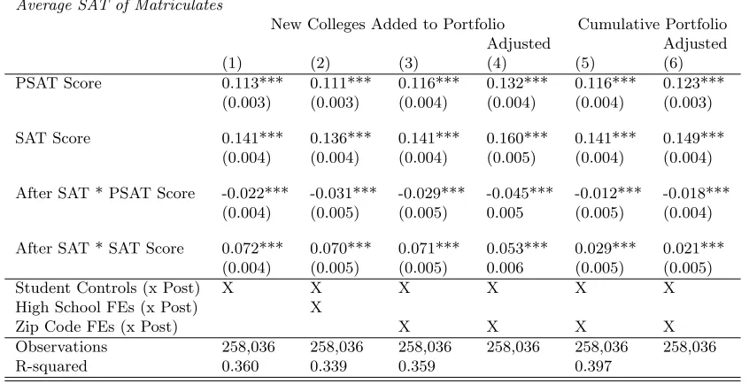
Columns (1)-(4) of Table 3 present the results of specification 13 for new colleges added to the portfolio. The estimates are consistent with updating in response to new information. Students place greater weight on the SAT score after it is revealed and reduce the weight placed on the PSAT. In column (1), which includes a rich set of student characteristic controls, the point
32
Note that by interacting observable characteristics with the post-exam indicator, we account for changes to college portfolio composition that are common across students who have the same demographic characteristics, household resources, and who live in the same zip code or attend the same high school. In line with the employer learning literature, we present results using a linear functional form for SAT and PSAT to ease interpretation. Allowing these variables to enter in a flexible polynomial leads to qualitatively similar results.
33A natural alternative is a first-differenced specification in which the change in the college portfolio is regressed on
the change in the score (P SAT−SAT). We prefer a difference-in-differences design because it does not assume that changes in the SAT and PSAT are given equal weight by the student (i.e. that a one point decrease in PSAT scores generates that same effect as a one point increase in SAT score), though in practice the results should be similar. Further, this design is naturally extended to the case of two-time takers.
34
Such factors could include performance in high school, participation in test preparation classes, or changes in motivation.
35This test is especially compelling because the colleges selected after the first SAT are often selected as free score
estimates suggest a 100 point increase in SAT score leads to a 7 point increase in the selectivity of the application portfolio. Given the scaling of the SAT and the distribution of SAT scores among college matriculates, this roughly corresponds to a one standard deviation increase in SAT score leading to a 0.12 standard deviation in college selectivity. This point estimate is roughly unchanged when we include zip code fixed effects in column (2) and high school fixed effects in column (3); in each case interacted with the period indicator to account for changes in portfolio composition that are common to a school or community.36
The magnitude of the effect represents the effect of the information shock (π1Λ) less attenuation that occurs if students anticipate their scores (i.e.
γ1γ4φ1). Thus this result can be viewed as a lower bound of the causal effect of new information
on the college application decision.37
In the case of two-time takers, we estimate and adjust for this attenuation explicitly and find little evidence of score anticipation.
Students may systematically employ strategies that vary with time, such as selecting colleges more or less ambitiously during the pre- and post-exam periods. If these strategies are shifts in levels common across all students then they will not affect the estimates – the indicator for the period will absorb the change in levels. However, if strategies reflect a scaling up or down of portfolio quality, then they necessarily vary across student aptitude. Following the approach outlined in Section 3.3, we account for this by regressing the outcome of interest on information available to the student (i.e. the PSAT and demographic characteristics) interacted with an indicator for each time period. We then calculate Ωt, the time-varying relationship between ability and portfolio choice as the ratio
between the return to ability in the final period to return to ability in periodt.38 Thus our ability covariates have a roughly time-constant relationship to our adjusted portfolios yt
Ωt. The estimates
of Ωtpresented in Appendix A indicate that higher ability students tend to be more aggressive with
their post-exam applications. Thus adjusting for time-varying strategies results in slightly smaller estimates of student response to new SAT information, as shown in column (4).39
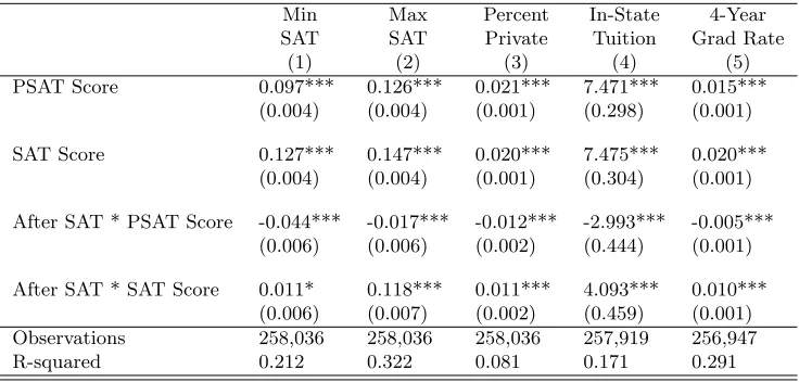
In columns (5)-(6) we measure the effect of student updating in terms of the cumulative selectivity of the portfolio. These results also suggest that students update in response to new information. After adjusting for time-varying strategies, our point estimates suggest that a 100 point positive shock to SAT score leads to an increase in the selectivity of one’s application portfolio of 2.1 SAT points. There is a similar pattern of effects when considering other measures of portfolio composition as shown in Table 4. The least selective college selected after the score is revealed does not appear to be sensitive to the score shock, but the most selective is quite sensitive. This is consistent with a case in which students apply to a safety college regardless of new information but
36Section 4.4 examines the estimates when using the joint sample of one and two-time takers. The resulting point
estimate of 0.055 is similar to the estimate for one-time takers only. Note that our preferred results are based on the split samples as they allow us to consider repeated instances of within-student updating for those who take the exam multiple times.
37
As discussed in the previous section, measurement error in SAT scores, and our rich set of student controls would suggest thatγ1γ4φ1 is small, and thus our estimate may not significantly understate the causal effect.
38
As the data include multiple time-invariant measures of aptitude, there are multiple possible estimates of Ωt. We estimate Ωt using the PSAT, but the results are not sensitive to selecting other measures or using an average.
39
only apply to a reach college if they experience a positive shock. Higher SAT score shocks result in students selecting a higher fraction of private colleges, colleges with higher average tuition, and colleges with higher graduation rates.40
For example, students who score 100 points higher on the SAT appear to apply to colleges with in-state tuition that is 400 dollars greater per year. Average in-state tuition for public universities during this period is 6,900 dollars, while average tuition across all universities is 13,250 dollars. The estimates for each characteristic of the portfolio reflect decreased weight placed on the PSAT after the SAT score is revealed. Strategy adjusted estimates for each outcome are presented in Appendix A. They closely mirror the unadjusted estimates in terms of both sign and magnitude, indicating that the results are not due to stronger students employing systematically different application patterns.
4.2 Two-Time Takers: Updating
Students who take the SAT more than one time provide especially compelling evidence of updating. In this context, the first and second information shocks are both generated by an SAT score, so there is no concern that students perceive the exams as fundamentally different in terms of importance or information content. Observing the responses to multiple shocks necessarily increases the credibility of estimates, as the probability that some unobserved, time-varying confounder would coincide with the treatment on multiple occasions is quite low. Further, the second score acts as a natural test of bias during the period when only the first score has been revealed.
Students who take the SAT twice receive two information shocks and send reports during three periods. Thus the specification is,
yit= β0+β1si+β2z1i+β3z2i+β4✶t=1+β5✶t=2 (14)
+β6si✶t=1+β7z1i✶t=1+β8z2i✶t=1
+β9si✶t=2+β10z1i✶t=2+β11z2i✶t=2+ǫit
where z1i and z2i are the student’s first and second SAT scores. The coefficient β7 represents
B10, the change in weight the student gives to the first SAT after the score is revealed, and β11
representsC20 the change in weight the student gives to the second SAT after it is revealed. The
coefficientsβ6 andβ9 representA10 andA20, the changes in weight given to the PSAT as each SAT
score is revealed. The coefficient on the second SAT when only the first SAT has been revealed, β8, is a measure of the extent to which students anticipate their scores using unobservables. Thus
interpreting magnitudes for multiple test takers is especially appealing. As shown in Section 3.2, B10−C10=π1Λ. Thus, the estimated effect of new information is β7−β8.
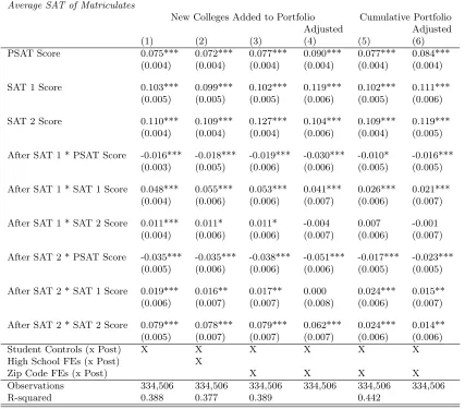
The results in Table 5 provide compelling evidence that students incorporate new information from each score. Beginning with newly selected colleges in columns (1)-(4), we see that after the first SAT score is revealed, the portfolio is less sensitive to the PSAT, reducing the coefficient by
40
0.02, and is more sensitive to the first SAT, increasing the coefficient by 0.05. Likewise, when the second SAT score is revealed, the portfolio discounts the PSAT even more, with a coefficient of -0.035, and a large change for the second SAT score, an increase in the coefficient of 0.078. The magnitude of the adjustments toward the first and second SAT scores as they are revealed are similar to the estimates of updating for one-time takers in the previous section. Cross-sectional difference for two time takers are 19 points for the first exam and 18 points for the second exam, again indicating that causal estimates of updating are about one-third of the differences observed in the cross-section.
As explained above, the coefficient on the second SAT when only the first SAT has been revealed provides a direct measure of attenuation bias due to students anticipating future scores. Once adjusting for time-varying strategies in column (4), we find that the coefficient is negative as expected.41
Importantly, the estimate is small and statistically insignificant. That is, we do not find evidence that students are able to anticipate their scores in such a way that it significantly biases the estimates. This is consistent with the noisy within-student distribution of scores in Section 2 and our inability to accurately predict them.
We compute the effect of the first SAT less the estimated effect of anticipation,β7−β8. With
this adjustment, a 100 point positive SAT score shock is estimated to cause a student to increase her college portfolio selectivity by 4.5 points. Note that the pattern of effects is similar when adjusting or not adjusting for strategy. Also of interest is the estimated response to the shock generated by the second SAT score. The estimates indicate that a 100 point higher score on the second SAT increases portfolio selectivity by 6.2 points. In contrast, students do not appear to use information from the first SAT in choosing new colleges after receiving the second SAT score. That is, students rely most heavily on new information when adjusting their portfolios. This suggests that the final portfolio will reflect both the first and second SAT.
The estimated effects of updating for the cumulative portfolio are presented in columns (5) and (6). After the first score has been revealed and prior to the second score being revealed (After SAT 1), only the first score is reflected in the portfolio. Adjusting for time-varying strategies, we see that a 100 point shock on their first SAT score causes students to adjust their portfolio upward by 2 points. Note that the bias generated by anticipation is only 0.1 points, as indicated by the coefficient on the second score. After both exams have been revealed to the student (After SAT 2), the first and second score have identical effects on the cumulative portfolio. That is, students appear to select new colleges in such a way that the final portfolio reflects both the first and second scores equally.
Specification (6) provides evidence of two predictions from the model. First, if SAT scores are i.i.d. draws conditional on ability from a students perspective, then they should be given equal weight prior to either being revealed in period 0. The estimated coefficients are 0.111 and 0.119,
41
respectively, and a formal test fails to reject that they are equal. Likewise, after both scores are revealed, they should be given equal additional weight for the cumulative portfolio. Again, the estimates are very similar with values of 0.015 and 0.014 and are not statistically different.
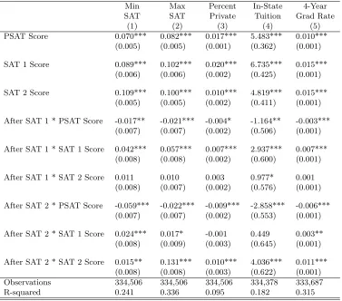
Table 6 presents alternate measures of portfolio composition.42
We again observe that the increase in selectivity stems primarily from the most selective colleges, with the least selective colleges remaining similar regardless of the shock. A 100 point increase in the first SAT score results in a portfolio with in-state tuition that is 300 dollars higher. Likewise, a positive score shock of 100 points on the second SAT produces an increase of 400 dollars, which corresponds to 6 percent of average in-state public tuition at four-year colleges. Positive information shocks result in students selecting colleges that have higher four-year graduation rates and a larger fraction of the portfolio consisting of private colleges. These findings are supported by specifications that adjust for time-varying strategies that are correlated with aptitude as shown in Appendix A. Of particular note is that relative to the pre-score period, only revealed scores are significantly incorporated into portfolio choice in each period. This strongly supports the hypothesis that students incorporate new information into portfolio choice and that they do not anticipate future scores using unobservables.
4.3 Heterogeneity in Updating
Student responses to new information may vary with gender, race, household resources, or the nature of the information shock. Those from higher or lower income households may respond more or less to new information. For example, students whose parents are unfamiliar with the college application process may respond less to a change in information if they apply to a fixed set of local colleges. Conversely, lower incomes students may respond more if they rely on having multiple admissions offers in order to negotiate for greater financial aid, or if the SAT substitutes for other forms of college counseling. The results in Table 7 indicate that students of all races and income ranges update significantly. A specification with interacted effects indicates that black students update more than white students, but that there are no significant differences across income groups. Though male students have slightly larger coefficients than female students, the differences in updating are not statistically significant. Perhaps most interestingly, students who receive positive shocks, where the SAT exceeds the predicted SAT, appear to be more responsive than students who receive negative shocks.43
This is consistent with the finding that the change in portfolio quality was primarily driven by the most selective college selected. Students may apply to safer schools regardless of their performance on the SAT, but only those who receive unexpected positive news choose to add more selective colleges to their portfolios.
Table 8 presents estimates by subgroup for two-time takers. All groups exhibit a consistent pattern with portfolios reflecting new information from the first SAT and second SAT as it is revealed to the student. Newly revealed first scores are highly significant and yet to be revealed
42As with the single test takers, we estimate these effects for newly selected colleges. Results using the cumulative
portfolio yield a similar pattern of results.
second SAT scores are not. This supports the hypothesis that no subgroup of students anticipates future scores in a significant way. For example, there is no evidence that higher income students appear to more accurately anticipate score shocks due to test prep classes. Again, the results do not suggest strong heterogeneity. Only two of the findings for one-time takers appear to carryover to students who take the exam twice: male students update more than female students after the first and second scores are released, which is statistically significant in this case; and those who receive two positive shocks update more than those who receive two negative shocks.
4.4 Extensive Margin Retaking and Score Reports
There are two extensive margins of interest: taking the exam once or twice; and sending additional reports after a score is revealed. We explicitly examine how student and household characteristics and the size of the SAT information shock appear to affect these two margins. To abstract from selection into retaking the exam, we merge one and two-time takers and replicate the primary design. We also estimate a lower bound estimate by assuming that all students who do not send additional reports did not update their beliefs.
Columns (1) and (2) of Table 9 indicate that students whose SAT score are lower than their PSAT scores are more likely to retake the exam, while those whose SAT score exceeds their PSAT scores are less likely to retake it.44
However, the magnitudes of these estimates are relatively modest, with a 100 point negative shock only increasing the retake rate by 2 percentage points and a 100 point positive shock decreasing the rate by 5 percentage points. By comparison, students from the highest income category are 9 percentage points more likely to take the exam than those in the lowest income category. One- and two-time takers are treated separately in the empirical analysis and result in similar patterns of estimates. To ensure that separating the sample on this margin is not biasing the estimates, we present estimates for the joint sample in Table 10. The results indicate that a 100 point test score shock causes a 5.5 point increase in the average score of matriculates in the college portfolio. This is consistent with the separate estimates presented in Sections 4.1 and 4.2.
Because reports must be sent after the exam in order to measure updating, the results are local to students who send more than the four free reports. While this is not a threat to the internal validity of the design, it does affect the interpretation of the estimates. Specifically, students in the sample used for analysis may have different socio-economic characteristics and may be more or less sensitive to new information than the population of all SAT takers. The decision to have more than four colleges in one’s portfolio may be determined by factors unrelated to the newly revealed score, such as household income or college readiness, or it may be a response to the amount that beliefs are updated in response to the score shock.
As shown in columns (3) and (4) of Table 9, students from higher income households and students with high grade point averages in high school are significantly more likely to send additional
44
score reports.45
Thus these students are over-represented in the sample. In contrast, the estimates reveal little evidence that students who update the most are more or less likely to send additional score reports. Specifically, the coefficient on the magnitude of the information shock, approximated by the absolute value of the difference between the SAT and PSAT score, indicates that a 100 point shock changes the probability of sending additional reports by less than one percentage point.46
This suggests that the amount of updating a student experiences as a result of the exam does not significantly affect the number of colleges in her portfolio.47
Thus the number of colleges a student includes in her portfolio appears to be primarily a function of characteristics such as household income and performance in high school, and is only marginally affected by updating in response to the score shock. Thus we have no evidence that the estimates in the analysis are systematically larger or smaller than those for the population as a whole. Nonetheless, we estimate the lower bound by assuming that all students who do not send additional reports did not update their beliefs. In practice, this is done by replacing missing post-exam portfolios with pre-exam portfolios. The resulting estimates are presented in columns (2) and (3) of Table 10. While these are mechanically smaller than the primary estimates, they nonetheless exhibit the same pattern of updating.
5
Conclusion
Relatively little is known about the extent to which students update their human capital decisions in response to new information about their aptitude. For example, it is unknown if such information can significantly close the gap between students with similar aptitude but from households with differing levels of resources. Research in this area is challenging due to the fact that many decisions are observed one time. The few studies that have made progress to this end have elicited beliefs using repeated surveys. This paper exploits a unique policy in conjunction with administrative data to overcome this issue in the context of college application portfolios. Specifically, we observe students selecting colleges to be in their portfolios before and after receiving SAT scores.
We find consistent evidence that students adjust their college application portfolios in re-sponse to new information about their aptitude and the strength of their applications. Information shocks associated with the SAT cause students to apply to more selective colleges that charge higher tuition and have higher graduation rates. After SAT scores are revealed, students rely less on prior
45
A one point increase in grade point average (on a 4 point scale) is correlated with an 8 percentage point higher probability of adding colleges to a student’s portfolio. Students from households with income exceeding 100,000 dollars are 5 percentage points more likely to send additional reports than a student from a household with income of less than 50,000 dollars.
46
In terms of the overall number of reports sent to colleges, a 100 point score shock is estimated to increase the size of the portfolio by 0.04 score reports.
47
sources of information such as the PSAT. This is apparent both for students who take the exam one time and thus experience one information shock and students who take the exam twice and experience two information shocks.
REFERENCES
Abramitzky, Ran, and Victor Lavy. 2014. “How Responsive is Investment in Schooling to Changes in Redistributive Policies and in Returns?” Econometrica 82(4): 12411272.
Altonji, Joseph G. 1993. “The Demand for and Return to Education When Education Outcomes are Uncertain.” Journal of Labor Economics 11(1): 48-83.
Altonji, Joseph G., and Charles R. Pierret. 2001. “Employer Learning and Statistical Discrimination.”
The Quarterly Journal of Economics 116(1): 313-350.
Altonji, Joseph G., Erica Blom, and Costas Meghir. 2012. “Heterogeneity in Human Capital Investments: High School Curriculum, College Major, and Careers.” Annual Review of Economics 4: 185-223. Arcidiacono, Peter, Esteban Aucejo, Arnaud Maurel, and Tyler Ransom. 2015. “College Attrition and the
Dynamics of Information Revelation.” Working Paper.
Arcidiacono, Peter, Patrick Bayer, and Aurel Hizmo. 2010. “Beyond Signaling and Human Capital: Education and the Revelation of Ability.” American Economic Journal: Applied Economics 2(4): 76-104.
Arcidiacono, Peter, V. Joseph Hotz, and Songman Kang. 2012. “Modeling College Major Choices Using Elicited Measures of Expectations and Counterfactuals.” Journal of Econometrics 166(1): 3-16. Attanasio, Orazio P., and Katja M. Kaufmann. 2009 “Educational Choices, Subjective Expectations, and
Credit Constraints.” NBER Working Paper 15087.
Avery, Christopher, and Thomas J. Kane. 2004. “Student Perceptions of College Opportunities: The Boston COACH Program.” In College Choices: The Economics of Where to Go, When to Go, and How to Pay For It, ed. C. Hoxby, 355-394. Chicago: University of Chicago Press.
Behrman, Jere R., Mark R. Rosenzweig, and Paul Taubman. 1996. “College Choice and Wages: Estimates Using Data on Female Twins.” The Review of Economics and Statistics 78(4): 672-685.
Bettinger, Eric, Bridget Terry Long, Philip Oreopoulos, and Lisa Sanbonmatsu. 2012. “The Role of Application Assistance and Information in College Decisions: The H&R Block FAFSA Experiment.”
The Quarterly Journal of Economics 127(3): 1205-1242.
Black, Dan A., and Jeffrey A. Smith. 2006. “Estimating the Returns to College Quality with Multiple Proxies for Quality.” Journal of Labor Economics 24(3): 701-728.
Bond, Timothy N. and Kevin Lang. 2013. “The evolution of the Black-White test score gap in Grades K3: The fragility of results.” Review of Economics and Statistics, 95 (5): 1468-1479.
Bond, Timothy N. and Kevin Lang. 2014. “The Sad Truth About Happiness Scales.” NBER Working Paper 19950.
Bulman, George. 2015. “The Effect of Access to College Assessments on Enrollment and Attainment.”
American Economic Journal: Applied Economics 7(4): 1-37.
Card, David, and Alan B. Krueger. 2005. “Would the Elimination of Affirmative Action Affect Highly Qualified Minority Applicants? Evidence from California and Texas.” Industrial and Labor Relations Review 58(3): 414-434.
Carrell, Scott and Bruce Sacerdote. 2012. “Late Interventions Matter Too: The Case of College Coaching in New Hampshire.” NBER Working Paper 19031.
Chade, Hector, Gregory Lewis, and Lones Smith. 2014. “Student Portfolios and the College Admissions Problem.” Review of Economic Studies 81(3): 971-1002.