Negative binomial quasi likelihood inference for general integer valued time series models

Munich Personal RePEc Archive

Negative binomial quasi-likelihood

inference for general integer-valued time

series models

Aknouche, Abdelhakim and Bendjeddou, Sara and Touche,

Nassim

Faculty of Mathematics, USTHB, Algeria, Mathematics

Department, Qassim University, Saudi Arabia, Department of

Operational Research, Faculty of Exact Sciences, University of

Bejaia, Bejaia, Algeria

6 December 2016

Online at

https://mpra.ub.uni-muenchen.de/83082/

Negative binomial quasi-likelihood inference for

general integer-valued time series models

Abdelhakim Aknouche , Sara Bendjeddou* and Nassim Touche*

December 2, 2017

Abstract

Two negative binomial quasi-maximum likelihood estimates (NB-QMLE’s) for a

general class of count time series models are proposed. The …rst one is the pro…le

NB-QMLE calculated while arbitrarily …xing the dispersion parameter of the negative binomial likelihood. The second one, termed two-stage NB-QMLE, consists of four stages estimating both conditional mean and dispersion parameters. It is shown that the two estimates are consistent and asymptotically Gaussian under mild conditions. Moreover, the two-stage NB-QMLE enjoys a certain asymptotic e¢ciency property provided that a negative binomial link function relating the conditional mean and conditional variance is speci…ed. The proposed NB-QMLE’s are compared with the Poisson QMLE asymptotically and in …nite samples for various well-known particular classes of count time series models such as the (Poisson and negative binomial) Integer-valued GARCH model and the INAR(1)model. Applications to two real datasets are given.

Faculty of Mathematics, University of Science and Technology Houari Boumediene. Mathematics de-partment, Qassim University.

y_{This material is a long version of a forthcoming paper (Aknouche etal,2017) to be published inJournal}

Keywords and phrases: Integer-valued time series models, Integer-valued GARCH, Integer-valued AR, Generalized Linear Models, Quasi-likelihood, Geometric QMLE, Negative Binomial QMLE, Poisson QMLE, consistency and asymptotic normality.

1. Introduction

Integer-valued time series such as count and binary data are well observed in a broad range

of applications (e.g. economics, …nance, epidemiology, medicine, telecommunications...).

They are characterized by some stylized facts such as small values, overfrequency of zeros,

locally constant behavior, overdispersion, positive autocorrelation structure, and asymmetric

marginal distributions (see e.g. Kedem and Fokianos, 2002; McKenzie, 2003; Fokianos,

2012; Cameron and Trivedi, 2013; Silva, 2015; Davis et al, 2016). It is well documented that continuous-valued time series models such as ARMA-like processes are inappropriate

for modeling such integer-valued series. This is why considerable interest has been paid in

recent decades to alternative integer-valued time series models. Numerous models have been

introduced so it appears di¢cult to classify them. However, two major classes of

valued models have played a central role. The …rst one is the class of models based on

integer-valued regressions such asgeneralized ARMA (GARMA) models, Poisson autoregression and especially PoissonInteger Generalized Conditional Heteroskedastic (INGARCH) models (e.g. Grunwald et al, 2000; Rydberg and Shephard, 2000; Benjamin et al, 2003; Heinen, 2003; Ferland et al, 2006; Fokianos et al, 2009; Zhu, 2011-2012a-2012b; Doukhan et al, 2012; Christou and Fokianos, 2014; Davis and Liu, 2016; Chen et al, 2016). The second class, however, concerns stochastic di¤erence equations involving the thinning operator where the best known example is the INteger AR (INAR) model (e.g. McKenzie, 1985-2003; Al-Osh and Alzaid, 1987; Silva, 2015; Bourguignon, 2016).

Ahmad and Francq (2016) recently introduced a more general integer-valued time

se-ries model that encompasses many models of the two aforementioned classes. This model

the in…nite past of the observed process. Important subclasses of this model are the

gen-eral Poisson autoregression (Doukhan et al, 2012; Doukhan and Kengne, 2015; Kengne,

2015), the INGARCH model and the INAR model. Ahmad and Francq (2016) established

consistency and asymptotic normality of thePoisson quasi-maximum likelihood estimate (P-QMLE), which is calculated as if the conditional distribution of the model were Poissonian.

The P-QMLE has in fact many advantages: i) …rst, it is robust to misspeci…cation of the

true conditional distribution whenever the conditional expectation is well speci…ed. This is

due to the fact that the Poisson likelihood belongs to the linear exponential family (White,

1982; Gourieroux et al, 1984a). ii) Second, it is asymptotically e¢cient when the true con-ditional distribution of the model is Poissonian. iii) Third, when the concon-ditional variance

and conditional mean of the model are proportional, the P-QMLE is asymptotically

e¢-cient in the class of all QMLE’s whose likelihood belongs to the linear exponential family

(see Gourieroux et al, 1984a). The latter proportionality between the conditional mean and conditional variance is usually called the PoissonGeneralized Linear Model (henceforth GLM) variance assumption (or link function). Despite these advantages, it is known that the Poisson model is less ‡exible in modeling overdispersed series than a model based on an

overdispersed conditional distribution such as the negative binomial one (e.g. Christou and

Fokianos, 2014; Zhu, 2011). Therefore, it is likely that the P-QMLE does not reach its full

asymptotic e¢ciency in the presence of overdispersed data which are frequently observed in

practice. Thus a QMLE calculated using an overdispersed likelihood while belonging to the

linear exponential family would be an interesting complementary to the P-QMLE.

For the model considered by Ahmad and Francq (2016), we propose two variants of the

negative binomial QMLE (NB-QMLE). These estimates are calculated on the basis of the negative binomial likelihood, belonging to the linear exponential family. The …rst one we

call "pro…le NB-QMLE" (pNB-QMLE) consists in maximizing the negative binomial

likeli-hood over the conditional mean parameter letting the corresponding dispersion parameter

arbitrarily …xed. In particular, when the latter parameter equals one, the resulting

however, consists of four stages: a two-stage NB-QMLE to estimate the conditional mean

parameter of the model and a two-stage weighted least squares estimate for the dispersion

parameter. For this, the underlying model should satisfy a negative binomial GLM link function involving the unknown dispersion parameter to be estimated. In the context of static integer-valued regression, a similar three-stage estimate was termed "quasi-generalized pseudo-maximum likelihood estimate" by Gourieroux et al (1984b) and "two-stage negative binomial quasi-maximum likelihood estimate" (2SNB-QMLE) by Wooldridge(1997). Adopt-ing the latter notation, the four-stage estimate we propose will be denoted by 2SNB-QMLE.

It will be shown under some mild assumptions that the two proposed estimates are

con-sistent and asymptotically Gaussian without fully specifying the conditional distribution of

the model. Moreover, under the negative binomial GLM link function, the 2SNB-QMLE is

asymptotically e¢cient in the class of all QMLE’s belonging to the linear exponential family,

including the P-QMLE.

The rest of this paper is outlined as follows. Section 2 presents the general

integer-valued time series model we deal with and some of its speci…c cases. Section 3 de…nes

some negative binomial QML criteria and establishes consistency and asymptotic normality

of the pNB-QMLE and the 2SNB-QMLE. As a result, Section 4 compares the asymptotic

variance of the proposed NB-QMLE’s with that of the P-QMLE under some speci…c GLM

assumptions as well as on particular classes of the general model. In particular, the Poisson

INGARCH model, thenegative binomial INGARCH model, the INAR(1)model, the Double Poisson INGARCH model and the Generalized Poisson INGARCH model are examined.

Moreover, these estimates are compared in …nite samples via some simulation experiments.

Application to the number of poliomyelitis cases in the United States (Polio data, Zeger,

1988) and the number of transactions of the Ericsson B stock (Transaction data, Fokianos

etal,2009; Christou and Fokianos,2014) under the negative binomial INGARCH framework are considered. Section 6 concludes while proofs of the main results are left to Section 7.

In what follows, we heavily use the following notations and conventions: All random

sym-bols Z _{= f:::; 1;0;1; :::g,} N _{= f0;1; :::g and} N ₌ N_{=f0g denote respectively the set of}

integers, the set of nonnegative integers and the set of positive integers. The notation

Y _P( ) means that the random variable Y has a Poisson distribution with parameter

>0. Similarly,X N B(r; p) means that X has the negative binomial distribution (also

called mixture Poisson-Gamma distribution). This distribution is given for any x ₂ N _by

fX(x) := P(X =x) = _x(_{! (}x+_rr₎)pr(1 p)x, where r > 0 is a positive real number called the

dispersion parameter,p₂(0;1)is a probability parameter, is the gamma function andx!

is the factorial of x. When r ₂ N _{has to be a positive integer, the factor} (x+r)

x! (r) may be

replaced by the binomial coe¢cient x+_xr 1 . In particular, whenr = 1we …nd the geometric

distribution and we simply write X _G(p). Following Cameron and Trivedi (1986, 2013),

the negative binomialK (NBK) conditional distribution given a -algebra B F is de…ned

by X_{j B N B} r 2 K;_rr22KK₊ where = E(Xj B) and r > 0. Two important cases

of the latter model are the negative binomial1 (NB1) conditional distribution corresponding

to K = 1 and the negative binomial2 (NB2) model for which K = 2. Finally, the symbols

a:s:

!

n!1,

p

!

n!1 and L

!

n!1 denote respectively almost sure convergence, convergence in

probabil-ity and convergence in distribution as n _{! 1} while op(1) and oa:s:(1) are respectively: a

term converging in probability to zero and a term converging almost surely (a:s:) to zero as

n_{! 1}.

2. A general class of count time series models

Let 0 2 Rm (m 2 N ) be an unknown "true" parameter and consider a measurable

positive real-valued function :N1 _{!(0;1). A general class of count time series}

mod-els, as proposed by Ahmad and Francq(2016), is given through an observable integer-valued

stochastic process _fXt; t2Zg, which is de…ned on ( ;F; P) with conditional expectation

speci…ed as follows

where _Ft F is the -algebra generated by fXt; Xt 1; :::g. Without any constraints on

(2:1), any discrete-time stochastic process satis…es(2:1). However, two restrictions are made

here. The …rst one is that _fXt; t2Zg is restricted to be integer-valued, i.e. with sample

space f0;1;2; :::g. The second one is that the function depends on the parameter 0 so

(2:1) is a parametric model. Letting

et:=et( 0) =Xt E(Xtj Ft 1);

model(2:1), which is de…ned through the conditional mean representation(2:1), may also be

written in the following stochastic di¤erence equation (or in innovation form, cf. Grunwald

etal, 2000)

Xt= (Xt 1; Xt 2; :::; 0) +et; t2Z: (2:2)

Equation (2:2), which is driven by the fFt; t 2Zg-martingale di¤erence fet; t2Zg,

ap-pears to be an in…nite nonlinear autoregression with an integer-valued solution_fXt; t2Zg.

In fact,model(2:1)-(2:2)is very general and encompasses many important classes of integer-valued time series models such as the (stable) Poisson INGARCH model (Grunwald et al,

2000; Rydberg and Shephard, 2000; Heinen, 2003; Ferland etal, 2006), the general Poisson autoregression (Doukhan etal,2012; Doukhan and Kengne, 2015; Kengne,2015), the stable negative binomial2 INGARCH model (Zhu, 2011; Christou and Fokianos, 2014; Davis and

Liu, 2016; Diop and Kengne, 2017) and the INAR model (McKenzie, 1985; Al-Osh and

Alzaid, 1987).

Note that the generality of model(2:1)stems not only from the general form of the

func-tion (:), but also from the fact that apart from the conditional mean, no other speci…cation

concerning the conditional distribution of the process _fXt; t 2Ng is required. However, it

is sometimes important to specify a link function relating the conditional variance and the conditional mean of model (2:1), i.e.

Var(Xtj Ft 1) =l(E(Xtj Ft 1)); (2:3)

func-tion is also called the GLM nominal variance assumption and is induced either by the con-ditional distribution of the model when it is fully speci…ed or by the structure of the model.

For example, when the conditional distribution corresponding to(2:1)is Poissonian with

pa-rameter t, which reduces to a special case of the general Poisson autoregression proposed by

Doukhan et al (2012), the Poisson GLM link function for model(2:1)is given by the linear forml(x) =x. A more general linear link function l(x) = 1 +_r1

0 x, for somer0 >0; is

in-duced by the negative binomial1conditional distribution, i.e. Xtj Ft 1 N B r0 t;_r0r0_t+t _t ,

r0 >0 (see Cameron and Trivedi,1986 and Section 4.1 below). Furthermore, the link

func-tion implied by the negative binomial2 conditional distribution, that is N B r0;_r0r₊0 _t , is

given by

l(x) = x 1 +x1

r0 ; r0 >0: (2:4)

When r0 = 1, we …nd the link function corresponding to the Geometric distribution. On

the other hand, a link function may be obtained even when the conditional distribution of

the model is misspeci…ed. In Section 4.1.4 we will see that the GLM link function for the

INAR(1) model is always an a¢ne function regardless of the conditional distribution of this

model.

In this paper we are interested in estimating the unknown conditional mean parameter 0

using a seriesX1; X2; :::; Xn (n 2N ) generated from (2:1). When a negative binomial2 link

function such as (2:3)-(2:4) is speci…ed we are also interested in estimating the dispersion

parameter r0. In fact, two instances of(2:1)are considered:

Case 1: Only the conditional mean (2:1) is speci…ed so that we only have to estimate

the conditional mean parameter 0.

Case 2: Equation (2:1) and the NB2 variance GLM assumption (2:3)-(2:4) are both

speci…ed so we have to estimate both 0 and r0.

A particularly important instance of Case 2 appears when the full conditional

distrib-ution of the model is speci…ed as a negative binomial2 one, i.e. Xtj Ft 1 N B r0;_r0r₊0 _t ,

where a special case is the NB2-INGARCH model (see Davis and Liu, 2016; Zhu, 2011;

For our estimation purposes we make the following regularity assumption on (2:1).

A0 The process fXt; t2Zg given by (2:1) is strictly stationary and ergodic.

For some particular classes of(2:1)such as the INGARCH and INAR models, assumption

A0may be expressed more explicitly as a stability condition on 0 (see Ahmad and Francq,

2016 and Section 4.1 below). Furthermore, when the conditional distribution of (2:1) is

Poissonian, Doukhan etal (2012) provided general conditions on the function in(2:1)for strict stationarity, ergodicity and weak dependence of the model. Their results were based

on Doukhan and Wintenberger (2008).

Now, given a generic parameter ₂ , the conditional mean function given by

(Xt 1; Xt 2; :::; ) := t( ); t2N;

clearly coincides with the conditional mean in(2:1)when = 0. It is unobservable because of

the unobservable valuesX0; X 1X 2; :::For any arbitrary …xed initial valuesXe0;Xe 1;Xe 2:::,

let

e_t( ) = Xt 1; Xt 2; :::X1;Xe0;Xe 1; :::; ; t 2N ;

be an observable proxy for t( ). The latter approximation serves in calculating various

QMLE-type of 0 we intend to study below.

3. Negative binomial QMLE’s

This Section considers two negative binomial QMLE’s of model (2:1) given a realization

X1; ::; Xn thereof. To describe these estimates consider Case 2 of model (2:1)-(2:4) with

unknown parameters 0 and r0. For any generic 2 and r > 0, the negative binomial

(log) likelihood, LeN B( ; r), based on the NB2 conditional distribution, N B r;_r+er

t( ) , is given by

e

LN B( ; r) =

1

n

n

X

t=1

elt( ; r); (3:1)

with elt( ; r) = rlog _r+er

t( ) +Xtlog

et( )

r+et( ) +

(Xt+r)

A negative binomial quasi-maximum likelihood estimate (NB-QMLE) of( 0; r0)is a

max-imizer of LeN B( ; r)over 2 and r >0.

Note, however, thatelt( ; r)given by(3:1)is not a member of the linear exponential

fam-ily in the sense of Gourieroux etal (1984a). So any maximizer of(3:1)might be inconsistent under misspeci…cation of the true conditional distribution of model (2:1), which constitutes

a serious limitation. In lieu of maximizing directly (3:1) and picking up the estimate

com-ponent corresponding to 0, we may consider a four-stage approach which is rather robust

to misspeci…cation of the true conditional distribution and which consists in:

i) Fixingr in(3:1)arbitrarily to any known positive number, sayr >0, and estimating

0 while maximizing (3:1) with respect to , giving a …rst-step QMLEbr .

ii) Estimating r0 under the GLM link function(2:3)-(2:4)using a weighted least squares

estimater_b1 while replacing 0 in the weight by its QMLE,br , obtained in i).

iii) Re-estimating 0 by maximizing a variation of (3:1) obtained while replacing r by

the estimate _br1 obtained in ii), givingbbr1.

iv) Re-estimating r0 using the same weighted least squares method in ii) but while

replacing 0 bybbr1 obtained in iii).

For a similar approach in the context of static count regression, see Gourieroux et al

(1984a; 1984b) and Wooldridge(1997; 2002). In the above …rst and third steps,

maximiza-tion of(3:1)is carried out with respect to lettingr …xed. So the last term in (3:1)may be

left out and (3:1)is simply replaced by the following "pro…le negative binomial likelihood" e

Ln;r( ) =

1

n

n

X

t=1

elt;r( ) withelt;r( ) =rlog _r+er

t( ) +Xtlog

et( )

r+et( ) : (3:2)

It should be noted that elt;r( ) in (3:2) rather belongs to the linear exponential family.

Therefore any maximizer of(3:2)with respect to would be robust to misspeci…cation of the

conditional distribution, whenever correctly specifying the conditional mean such as (2:1).

It turns out that for any …xed r > 0, Len;r( ) is the Wedderburn quasi-likelihood function

(Wedderburn,1974) based on the NB2 variance GLM assumption(2:3)-(2:4)(withr in place

On the other hand, if we considerCase 1of model(2:1)where only the conditional mean

is speci…ed, then only 0 has to be estimated and r in (3:1) can be set to any positive real

value. So maximization of (3:1) will only be done with respect to , which again amounts

to maximizing (3:2). In summary, for both Case 1 and Case 2, we have to maximize the pro…le (or Quasi-) likelihood(3:2)with respect to .

In the rest of this Section we shall study asymptotics of two QML-type estimates that

maximize(3:2)over ₂ . Section 3.1 examines consistency and asymptotic normality of a

maximizer of(3:2)for arbitrarily …xedr >0. The resulting estimate will be calledpro…le (or

marginal) NB-QMLE (pNB-QMLE). In Section 3.2, consistency and asymptotic normality of the four-stage estimate (seei)-iv)above) are established assuming the NB2 variance GLM

assumption (2:3)-(2:4) for an unknownr0 >0.

3.1. Pro…le negative binomial QMLE

Consider Case 1 of model (2:1). A pro…le negative binomial quasi-maximum likelihood estimate (pNB-QMLE) of 0 is any measurable solution of the following problem

b_r = arg max

2 Len;r( ) ; (3:3)

for some and some …xed known r > 0, where Len;r( ) is given by (3:2). When r = 1, b1

reduces to the geometric QMLE (G-QMLE) studied by Aknouche and Bendjeddou (2017).

The choice of (Xe0;Xe 1; :::) is of no asymptotic importance, but may in‡uence the accuracy

of estimate in …nite samples. In general, one assumes that Xe0 = x;Xe 1 = x; ::: with x

depending on the function or on the observations (see Ahmad and Francq, 2016). To

study consistency of the pNB-QMLE,br, we need the following assumptions:

A1 _7! t( ) is a:s: continuous; t( ) > c and et( )> c, a:s: for some c > 0.

A2 at a:s:

!

t!10 and atXt

a:s:

!

t!10 where at= sup 2 et( ) t( ) .

A3 E X_t <₁ for some >1.

A4 t( ) = t( 0) a:s: if and only if = 0.

Assumptions A1-A5 are standard and may be made more explicit for some particular

models of(2:1)(cf. Section 4.1). Similar assumptions were considered by Ahmad and Francq

(2016) for the strong consistency of their P-QMLE.

Theorem 3.1 Under (2:1) and A0-A5, br a:s:!

n!1 0; for all r >0: (3:4)

The latter result shows that, like the P-QMLE, the pNB-QMLE is robust to

misspeci…-cation of the true conditional distribution where only (2:1) has to be speci…ed. This is not

surprising as the pro…le negative binomial log-likelihood(3:2)belongs to the linear

exponen-tial family (see Gourieroux et al, 1984a).

We now examine the asymptotic normality of the pNB-QMLE. Let lt;r( ) be de…ned in

the same way aselt;r( )in(3:2)with t( ) in place ofet( ) and setLn;r( ) = 1_nPn_t=1lt;r( ).

Consider the following supplementary assumptions.

A6 The variables ct; ctXt; atdt; atdtXt and btdtXt are of order O(t ) a:s: for some

>1=2, where bt= sup ₂ e

2

t( )

2

t( ) ; ct= sup ₂

@(et( ) t( ))

@ and

dt= sup

2

max _e 1

t( )(r+et( ))

@et( )

@ ;

1

t( )(r+ t( ))

@ t( )

@ :

A7 The true 0 belongs to the interior of .

A8 The conditional variance vt( 0) := Var(Xtj Ft 1) = E(Xt2j Ft 1) 2t( 0) is a:s:

…nite.

A9 The derivatives @2 t( )

@ @ 0 and @2_e

t( )

@ @ 0 exist and are continuous, the matrices

Ir=E 2 vt( 0)

t( 0)(r+ t( 0))2

@ t( 0)

@

@ t( 0)

@ 0 and Jr=E _{t( 0)(r}1_{+ t( 0))} @ t( 0)

@

@ t( 0)

@ 0 ;

are …nite, and Jr is nonsingular for all r >0.

A10 There is a neighborhood V ( 0) of 0 such that E sup

2V( 0)

@2_l

t;r( )

@ @ 0

!

< ₁ for all

r >0.

Theorem 3.2 Under (2:1) and A0-A10,

p

n br 0 !L

n!1N 0; J

1

r IrJr1 for all r >0: (3:5)

Some remarks are in order:

- When the conditional distribution of the data generating process (2:1) is NB2 with

parameters r0 and _r0r₊0 _t, i.e. Xtj Ft 1 N B r0;_r0r₊0 _t , then (3:5) holds with Ir =

1

r0E

r0+ t( 0)

t( 0)(r+ t( 0))2

@ t( 0)

@

@ t( 0)

@ 0 . In particular, when r in (3:2)-(3:3) coincides with the

"true" r0 in (2:3)-(2:4) then Ir0 = 1

r0Jr0, so(3:5)becomes p

n br0 0

L

!

n!1 N 0;

1

r0J 1

r0 : (3:6)

- A weak result, which does not require specifying the full conditional distribution is that

under the following more generalnegative binomial2 GLM link function

Var(Xtj Ft 1) = 2E(Xtj Ft 1) 1 +_r1₀E(Xtj Ft 1) for some 2 >0; r0 >0; (3:7)

which generalizes (2:3)-(2:4),br0 is asymptotically e¢cient in the class of all QMLE’s in the

linear exponential family (see e.g. Gourieroux et al (1984a; 1984b) and Wooldridge (1997)

in the context of QML inference for static integer-valued regression models). In that case

we have

p

n br0 0

L

!

n!1N 0;

2_J 1

r0 : (3:8)

Note, however, that r0 is generally unknown and (3:6) and (3:8) does not hold unless r0 is

consistently estimated under (3:7) as we will see in the following subsection.

Now an important issue is to estimate the asymptotic variance of the pNB-QMLE.

Simi-larly to Ahmad and Francq(2016), a consistent estimate of the asymptotic varianceJ 1

r IrJr 1

of the pNB-QMLE,br, is Jbr 1IbrJbr 1 with

b

Ir = 1_n

n

X

t=1

Xt et(br)

et(br)(r+et(br))

2

@et(br)@et(br)

@ @ 0 : (3:9)

b

Jr = 1_n

n

X

t=1

1

et(br)(r+et(br))

@et(br)@et(br)

3.2. Two-stage negative binomial QMLE

Consider Case 2 of model (2:1)-(2:4) for which we study the aforementioned four-stage

procedure i)-iv). Here, the second and fourth steps are described in more details. Under the

GLM assumption (2:3)-(2:4), if we set

ut= (Xt t)2 E (Xt t)2 Ft 1 = (Xt t)2 1 + _r1₀ t t; (3:11a)

then E(utj Ft 1) = 0 and

(Xt t( 0))2 t( 0)

2

t( 0) = 0+

ut

2

t( 0); (3:11b)

where ₀ = 1

r0. Regression(3:11)is not ready to be used to estimate 0 since its regressand,

(Xt t( 0))2 t( 0)

2

t( 0) , depends on the unknown 0 and is then unobservable. If a consistent

estimate of 0, say b, is available then we may form the following modi…ed

(observable-regressand) regression

(Xt bt)

2 bt

b2_t = 0+ b

ut

b2_t; (3:12a)

where

b

ut= Xt bt

2

1 + _r1₀bt bt and bt= t b : (3:12b)

From(3:12a)a consistent estimate ofr0isbr, the inverse of the weighted least squares estimate

b of ₀ given by

b

r= _n1

n

X

t=1

(Xt bt)

2 bt

b2t

! 1

; _b=_br 1; (3:13)

where bt = et b . Note that the estimate rbwe use here is a dynamic adaptation of the

estimate proposed by Gourieroux et al (1984b) in the context of static negative binomial regression. Now, with (3:13) the following algorithm summarizes the four-stage approach

i)-iv) described above.

Algorithm 3.1 (Two-stage NB-QMLE)

Given a …xed known r >0, the two-stage NB-QMLE of ( 0; r0) in (2:1)-(2:4) consists

of a quadruple br ;br1;brb1;br2 , which is described by the following steps:

Step 1 Set br = arg max 2 Len;r ( ), a solution to the problem (3:3) while replacing r

Step 2 Set _b1 = _n1 P_tn₌₁ (Xt b1t)

2 b1t

b2_1t and br1 =b

1

1 .

Step 3 Let br_b1 = arg max 2 Len;br1( ) be a solution of the problem (3:3) while replacing

the generic r by r_b1. Get b2t=et bbr1 ; (1 t n).

Step 4 Set _b2 = _n1 P_tn₌₁ (Xt b2t)

2 b2t

b2₂t

and r_b2 =b21.

To get asymptotic properties of the quadruple br ;br1;brb1;br2 , note …rst that br is no

other than the pro…le NB-QMLE proposed in Section 3.1 whose asymptotic properties were

given by Theorem 3.1 and Theorem 3.2. So it remains to study the triple _br1;bbr1;rb2 ,

asymptotic properties of which are given by the following result.

Theorem 3.3 Under (2:1),(2:3)-(2:4) and A0-A10, b

r1

a:s:

!

n!1r0; (3:14a)

p

n(_{b1 0}) _!L

n!1 N 0; E

(Xt t( 0))2 t( 0)+_r1

0 2

t( 0) 2

4

t( 0)

!!

; _b2 A:D:= _b1;(3:14b)

b_br1 a:s:

!

n!1 0; (3:14c)

p

n b_br1 0

L

!

n!1N 0;

1

r0J 1

r0 ; (3:14d)

where A:D:= stands for equality in asymptotic distribution. A few broad conclusions can be drawn.

- Strong consistency of br_b1 directly follows from strong consistency ofbr (for all r > 0)

and _br1.

- The third-step estimate b_br1 is clearly more asymptotically e¢cient than the …rst-step

estimatebr .

- No supplementary moment assumptions apart those required byA0-A10are needed for

consistency and asymptotic normality of _b1. Other methods for estimating are available

(e.g. Christou and Fokianos, 2014), but they may involve higher order moment conditions.

- Asymptotic distribution of _br1 is areciprocal normal distribution, which is bimodal and

has no …rst moment.

re-estimate r0 using b2t and hence bbr1, which is more asymptotically e¢cient than br we

used in Step 2.

- A consistent estimate of the asymptotic variance 1

r0J 1

r0 of the third-step estimate,brb1,

is

1

b

r2Jb 1

b

r2 ; (3:15)

where Jbr_b2 is given by (3:10). Note that since here Ir=Jr, then(3:9)may also be used.

- A consistent estimate of the asymptotic variance of _b2 in (3:14b) is

1

n n

X

t=1

(Xt t(brb₁))

2

t(bbr₁)+_r1

0 2

t(bbr₁)

2

4

t(bbr₁) : (3:16)

- The outputs of the 2SNB-QMLE method are r_b2 = (b2) 1

andb_br1.

4. Comparison between the NB-QMLE’s and the

Pois-son QMLE

For the conditional mean parameter 0 of model (2:1), Ahmad and Francq(2016) proposed

a Poisson QMLE (P-QMLE), which is de…ned as a measurable solution to the following

problem

b_P = arg max

2 LeP;n( ) ; (4:1a)

where

e

LP;n( ) = 1_n n

X

t=1

et( ) +Xtlog et( ) : (4:1b)

Under similar assumptions to A0-A10, Ahmad and Francq (2016) showed consistency

and asymptotic normality of the P-QMLE with

p

n bP 0 !L

n!1N 0; J

1

P IPJP1 ; (4:2)

where IP = E vt2( 0)

t( 0)

@ t( 0)

@

@ t( 0)

@ 0 and JP = E _t(1₀₎@ _@t( 0)@_@t(00) . One important

prop-erty of the P-QMLE is its robustness to misspeci…cation of the true conditional distribution

to asymptotic relative e¢ciency for some well-known speci…c cases of(2:1)and also on some

particular GLM link functions of (2:3). We also compare these estimates in …nite samples

through some simulation experiments.

4.1. Comparison on asymptotic relative e¢ciency for speci…c

mod-els

4.1.1. The Poisson INGARCH model (Poisson autoregression)

The Poisson integer-valued GARCH (INGARCH(p; q)) process _fXt; t 2Zg, as proposed by

Rydberg and Shephard (2000) and Grunwald et al (2000), is de…ned to have a Poisson conditional distribution

Xtj Ft 1 P( t); t2Z; (4:3a)

with conditional mean t= t( 0) speci…ed as follows

t( 0) = !0 +

q

X

i=1

0iXt i+

p

X

j=1

0j t j( 0); (4:3b)

where 0 = !0; 01; :::; 0q; 01; :::; 0p

0

is such that !0 > 0; 0i 0, 0j 0. It is also

assumed that Xt is nondegenerate and that if p > 0 A 0(z) =

Pq

i=1 0izi and B 0(z) =

1 Pp_i=1 0izi have no common roots (cf. Ahmad and Francq, 2016). Ferland et al (2006)

showed that under the following stability condition

q

X

i=1

0i+

p

X

j=1

0j <1; (4:4)

the process fXt; t2Zg given by (4:3) is strictly stationary (see also Franke, 2010). The

ergodicity of the Poisson INGARCH(p; q)model(4:3)has been established …rst by Grunwald

etal (2000)forp= 0, by Fokianos et al (2009), Neumann (2011), Davis and Liu(2016)and Douc et al, (2013) for the case p = q = 1, and by Doukhan et al (2012) and Gonçalves et

al (2015) for general p and q. Under P_jp_{=1 0j} <1, the conditional mean t of the process

it is characterized by the following "identity" GLM link function

Var(Xtj Ft 1) = E(Xtj Ft 1). (4:5)

On the other hand, the P-QMLE of (4:3) reduces to the maximum likelihood estimate,

which is asymptotically e¢cient and is then more asymptotically e¢cient than the

pNB-QMLE. In particular IP = JP follows from (4:2) and (4:5). Furthermore, assumptions

A0-A10simplify in the case of the Poisson INGARCH model(4:3)as in Ahmad and Francq

(2016). For instance,A0is implied by (4:4)whileA1andA4follow from the linear form of

t in(4:3b). Since (4:4) entails the existence of moments of any order (Ferland et al, 2006)

thenA3andA8and A9are obviously satis…ed. A similar argument shows thatA2andA6

are satis…ed. As a result, Ir de…ned in A9 reduces to Ir = E 1

t( 0)(r+ t( 0))2

@ t( 0)

@

@ t( 0)

@ 0 .

Note …nally that the 2SNB-QMLE given by Section 3.2 is ill-de…ned in the present Poisson

INGARCH case since the Step 2 of Algorithm 3.1 is derived under the GLM assumption

(2:3)-(2:4), which is di¤erent from the link function (4:5) characterizing the Poisson

IN-GARCH model (4:3).

4.1.2. The negative binomial1-INGARCH model

Here we follow Cameron and Trivedi (1986, 2013) who proposed the negative binomialK

conditional distribution in the context of static integer-valued regression. We say that

fXt; t2Zg is a negative binomialK-INGARCH (NBK-INGARCH(p; q)) process if its

condi-tional distribution is a negative binomial one,

Xtj Ft 1 N B(rt; t); t 2Z; (4:6a)

with parameters

rt=r0 2t K and t = r0

2 K

t

r0 2t K+ t; (4:6b)

where K ₂ Z_{, r0 > 0 and t = t( 0) satis…es the INGARCH(p; q) representation (4:3b).}

Model (4:6) in whichE(Xtj Ft 1) = t satis…es the following GLM link function

which implies the process is conditionally overdispersed since Var(Xtj Ft 1)> E(Xtj Ft 1).

Now consider the NB1-INGARCH(p; q) model corresponding toK = 1, i.e.

Xtj Ft 1 N B r0 t;_r0r0_t+t _t N B r0 t;_r0r₊₁0 . (4:8a)

for which (4:7)reduces to the following linear form

Var(Xtj Ft 1) = 1 +_r1₀ E(Xtj Ft 1): (4:8b)

This is a strict generalization of the Poisson GLM condition (4:5) implied by the Poisson

INGARCH model. In view of (4:5) and (4:8b), the NB1-INGARCH model (4:8a) presents

some similarities with the Poisson INGARCH model (4:3). Indeed, we conjecture that the

NB1-INGARCH is strictly stationary with …nite second moment and ergodic under the same

stationarity condition (4:4) for the Poisson INGARCH model. Moreover, from (4:2) and

(4:8b), it follows under similar assumptions toA0-A10(see Ahmad and Francq,2016) that

p

n bP 0 !L

n!1N 0; 1 +

1

r0 E 1

t( 0)

@ t( 0)

@

@ t( 0)

@ 0

1 :

A more important result is that under the Poisson GLM condition(4:8b), it is easily seen that

the P-QMLE is asymptotically e¢cient in the class of all QMLE’s belonging to the linear

exponential family. So the P-QMLE is more asymptotically e¢cient than the pNB-QMLE

(see Gourieroux et al (1984a; 1984b) in the case of static integer-valued regression models where adaptation to the present dynamic case is trivial). In fact, under A0-A10 and in

view of (3:5) and (4:8b), the asymptotic variance of the pNB-QMLE, br, is in "sandwich"

form with Ir = 1 + _r1₀ E 1

t( 0)(r+ t( 0))2

@ t( 0)

@

@ t( 0)

@ 0 . Note …nally that like the Poisson

INGARCH case, the 2SNB-QMLE given by Section 3.2 is ill-de…ned.

4.1.3. The negative binomial2-INGARCH model

Consider the NB2-INGARCH(p; q)model corresponding to (4:6) with K = 2, i.e.

where r0 > 0 and t is given by (4:3b). The same parameter restriction for the Poisson

INGARCH is assumed here. Model (4:9) has been considered by Zhu (2011), Davis and

Liu (2016) and Christou and Fokianos (2014) who gave for p = q = 1 the following strict

stationarity condition

2

0 1 + r10 + 2 0 0+

2

0 <1;

with …nite second moment. The formulation of Zhu(2011) is in fact,

Xtj Ft 1 N B r0;₁₊1

t ; (4:10)

wherer0 2N is restricted to be a positive integer and t satis…es(4:3b). However, the latter

may be written in the form (4:9) while taking t = _r0t. For model (4:9), the link function

(4:7) clearly reduces to the NB2 GLM condition(3:7)(with 2 = 1), i.e.

Var(Xtj Ft 1) =E(Xtj Ft 1) 1 + _r1₀E(Xtj Ft 1) ; r0 >0; (4:11)

under which the 2SNB-QMLE is derived. Christou and Fokianos (2014) used the

Pois-son QMLE for estimating model (4:9) and proved its consistency and asymptotic

normal-ity with asymptotic variance in sandwich form like (4:2) where, in view of (4:4), IP =

1

r0E

(r0+ t( 0))

t( 0)

@ t( 0)

@

@ t( 0)

@ 0 . Ahmad and Francq (2016) showed how their assumptions of

consistency and asymptotic normality for the general model(2:1)simplify for model (4:9).

Concerning the pNB-QMLE, assumptionsA0-A10simplify forp=q= 1 as in the

Pois-son INGARCH case. A notable di¤erence is that one should assume the existence ofE(X4

t)<

1, a condition of which is given by Ahmad and Francq(2016). For generalpandq, a general moment condition seems di¢cult to obtain. Note that asIr = _r1₀E (₍r_r0₊+_tt₍(₀0₎₎))@ _@t( 0)@ _@t(00) ,

none of the pNB-QMLE and P-QMLE is asymptotically superior than the other, unless r0

would be known. In that case, one takes r = r0 and the resulting pNB-QMLE,br0, would

be asymptotically e¢cient. For instance, consider theGeometric INGARCH model which is a special case of the NB2-INGARCH model (4:9)in whichr0 = 1, i.e. Xtj Ft 1 G ₁₊1 _t :

For this model, the Geometric QMLE (G-QMLE), which is a particular case of pNB-QMLE

corresponding tor = 1, reduces to the maximum likelihood estimate and is then

However, wether or not r0 is known, the 2SNB-QMLE has the nice property of being

asymptotically e¢cient in the class of all QMLE’s belonging to the linear exponential family

(cf. Theorem 3.3). Hence, it is more asymptotically e¢cient than the P-QMLE.

Finally, it is worth noting that when K =2 f1;2g, the link function (4:7) corresponding

to the NBK-INGARCH model is di¤erent from both the Poisson GLM condition (4:8b) and

the NB2 variance assumption (4:11). Therefore, the 2SNB-QMLE is ill-de…ned and none of

P-QMLE and pNB-QMLE is asymptotically preferred than the other.

4.1.4. The INAR(1) model

A well-known particular case of (2:1) is the …rst-order integer-valued autoregressive model

(INAR(1)) proposed by McKenzie (1985) and Al-Osh and Alzaid (1987). This model has

the following form

Xt = 0 Xt 1+"t; t 2Z; (4:12)

wheref"t; t2Zgis an independent and identically distributed (iid) sequence of non-negative

integer-valued random variables with mean E("t) = !0 >0 and variance Var("t) = 20 >0.

The symbol denotes the binomial thinning operator (cf. Steutel and Van Harn, 1979)

de…ned for any non-negative integer-valued random variable X by 0 X =PXi=1Yi, where

fYi; i2Ng is aniid Bernoulli random sequence such thatP(Yi = 1) = 0 2(0;1). It is well

known that

E(Xtj Ft 1) = t( 0) = 0Xt 1+!0; with 0 = ( 0; !0)0;

and that assumption A0 reduces in term of 0 to 0 < 1 (cf. Al-Osh and Alzaid, 1987).

Furthermore, the INAR(1) model (4:12) obeys to the followinga¢ne GLM link function

Var(Xtj Ft 1) = 0(1 0)Xt 1+ 20 = (1 0)E(Xtj Ft 1) + 20 (1 0)!0: (4:13)

Note that if 20

!0 = 1 0 < 1, so that the innovation term "t would be underdispersed,

then the a¢ne link function(4:13) reduces to the linear Poisson GLM condition (4:8b) with

in the class of all QMLE’s belonging to the linear exponential family and hence it would be

more asymptotically e¢cient than the pNB-QMLE. Speci…cally,

p

n bP 0 !L

n!1 N 0;(1 0) E

1

t( 0)

@ t( 0)

@

@ t( 0)

@ 0

1

.

If, however, 20

!0 6= (1 0), then none of the two estimates P-QMLE and pNB-QMLE is more

asymptotically e¢cient than the other. Moreover, in all cases the 2SNB-QMLE is ill-de…ned.

4.1.5. The double Poisson INGARCH (DP-INGARCH) model

The double-Poisson INGARCH model as proposed by Heinen(2003) is de…ned by

Xtj Ft 1 DP( t; ) (4:14)

where t is given by (4:3b), > 0 and X DP( ; ) means that X has a double Poisson

distribution (cf. Efron, 1986) given by

P (X =x) = c( ; )e _xxxx e_x x; x=N_;

c( ; ) being a normalizing constant. It is well known (e.g. Ahmad and Francq, 2016)

that E(Xtj Ft 1) = t so the DP-INGARCH is a particular case of (2:1). It is especially

recommended for representing underdispersion. Ahmad and Francq conjectured that the

DP-INGARCH(1;1) is ergodic under the same condition(4:4)for the Poisson INGARCH(1;1).

Under that condition, assumptions A0-A10 may be made explicit in the same way as in

Ahmad and Francq(2016). Note that Var(Xtj Ft 1)is approximately equal to t= , which is

an approximation of the Poisson GLM variance assumption(4:8b). Therefore, the P-QMLE

is "approximately" more asymptotically e¢cient than the pNB-QMLE.

4.1.6. The generalized Poisson INGARCH model

A random variableXis said to have a Generalized Poisson (_GP) distribution with parameters

>0and 0 <1, that is X GP( ; ), if

The latter de…nition can be extended for <0. In order to model both conditional

overdis-persion and conditional underdisoverdis-persion, Zhu (2012a) introduced the generalized Poisson

INGARCH (GP-INGARCH) model as follows

Xtj Ft 1 GP( t(1 ); ); (4:15)

where t is given by(4:3b). Since E(X) = =(1 ), it is clear that the GP-INGARCH is

a particular case of (2:1). Gonçalves et al (2015) showed that the latter model is ergodic under the same condition as that of the Poisson INGARCH model. Ahmad and Francq

(2016) showed the consistency of the P-QMLE under similar conditions to A0-A10. These assumptions hold under the ergodicity condition (4:4). Note that the conditional variance

has a rather complicated expression of the conditional mean, which is di¤erent from the

Poisson and the NB2 GLM variance assumptions. Therefore, none of the two estimates

P-QMLE and pNB-P-QMLE is asymptotically preferred than the other. For the same reason,

the 2SNB-QMLE is ill-de…ned.

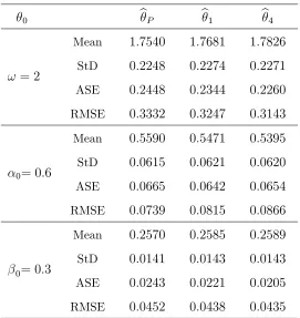
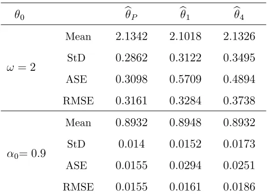
4.2. Comparison in …nite samples

We now examine the …nite-sample performance of the proposed NB-QMLE’s on simulated

series with sample size n = 1000. These series are generated from six instances of (2:1),

namely:

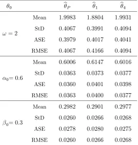
i) The Poisson INGARCH(1;1) model (4:3)with parameter 0 = (2;0:6;0:3)0 (cf. Table

4.1).

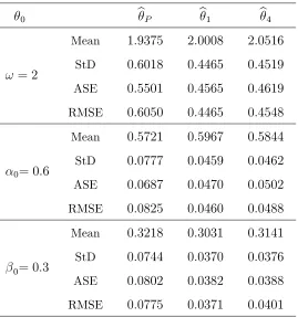
ii) The geometric INGARCH(1;1) model corresponding to (4:9) with r0 = 1 and 0 =

(2;0:3;0:6)0 (cf. Table 4.2).

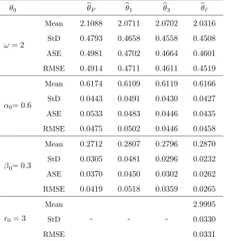
iii) The NB2-INGARCH(1;1) model (4:9)with parameters r0 = 3 and 0 = (2;0:6;0:3)0

(cf. Table 4.3).

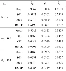
iv) The DP-INGARCH(1;1) model (4:14) with = 2 and 0 = (2;0:6;0:3)0 (cf. Table

4.4).

4.5).

vi) The (Poisson) INAR(1)model(4:12)with = 0:9and"t P(2), that is 0 = (2;0:9)0

(cf. Table 4.6).

Three QMLE’s are compared on these models: i) The Poisson QMLE (bP, Ahmad and

Francq,2016) given by(4:1), ii) the Geometric QMLE,b1, corresponding to(3:3)withr = 1,

and iii) the pro…le negative binomial QMLE, b4; given by (3:3) with r = 4. For the NB2

-INGARCH(1;1) model (4:9) we also run the two-stage NB-QMLE, br ;br1;brb1;br2 , given

by Algorithm 3.1. These estimates are calculated using 500 Monte Carlo replications for

the three mentioned models. In implementing the NB-QMLE’s, we used the same devices.

The starting parameter value, (0) = !(0)_; (0)_; (0) 0_{, of the nonlinear optimization routine}

(3:3) is set to the value obtained while preliminarily running a pNB-QMLE starting from

an initial parameter ( 1) = (2;0:3;0:6)0 and r( 1)_{= 3. The unobservable starting valuesX} 0

and 0( ) of the INGARCH(1;1) equation are estimated respectively by

e

X0 =X and e0( ) = !₁+ X 'E( t( )) for = (!; ; )0 2 ; (4:16)

where X is the empirical mean of the seriesX1; :::; Xn. Concerning Algorithm 3.1, which is

only applied in the case of the NB2-INGARCH model (4:9), we need to estimate the initial

dispersion parameter r . For this we mimic the negative binomial2 GLM assumption(4:11),

taking r to be a solution to the equation, S2 _{=X 1 +} 1

r X ; i.e.

r = (X)

2

S2 _X; (4:17)

whereS2 _{is the sample variance of X}

1; :::; Xn. Of course, there is no theoretical justi…cation

for this choice. We have just replaced in(4:11)the conditional variance and conditional mean

by their unconditional sample counterparts. For that choice, the seriesX1; :::; Xn should be

overdispersed (i.e. S2 _{> X), otherwise r would be negative, which is not valid.}

Mean of estimates, their standard deviation (StD), their Asymptotic Standard Errors

(ASE) and their empirical Root Minimum Square Error (RMSE) over the 500 replications

are reported in Tables 4.1-4.6. The RMSE of an estimate b of 0 is calculated from the

replications. The ASE’s are obtained from the asymptotic variances of the NB-QMLE’s

given by Theorem 3.2 and Theorem 3.3, and that of the P-QMLE (cf. Ahmad and Francq,

2016 and Section 4.1 above).

0 bP b1 b4

!= 2

Mean StD ASE RMSE

1:9983

0:4067

0:3979

0:4067

1:8804

0:3991

0:4017

0:4166

1:9931

0:4094

0:4041

0:4094

0= 0:6

Mean StD ASE RMSE

0:6006

0:0363

0:0360

0:0363

0:6147

0:0373

0:0401

0:0400

0:6016

0:0377

0:0398

0:0377

0= 0:3

Mean StD ASE RMSE

0:2982

0:0260

0:0278

0:0260

0:2901

0:0266

0:0280

0:0266

0:2977

0:0268

0:0275

0:0268

Table 4.1: Mean, standard deviation, asymptotic standard error and empirical RMSE ofbr (r = 1;4) andbP for Poisson INGARCH(1;1)

0 bP b1 b4

!= 2

Mean StD ASE RMSE

1:9375

0:6018

0:5501

0:6050

2:0008

0:4465

0:4565

0:4465

2:0516

0:4519

0:4619

0:4548

0= 0:6

Mean StD ASE RMSE

0:5721

0:0777

0:0687

0:0825

0:5967

0:0459

0:0470

0:0460

0:5844

0:0462

0:0502

0:0488

0= 0:3

Mean StD ASE RMSE

0:3218

0:0744

0:0802

0:0775

0:3031

0:0370

0:0382

0:0371

0:3141

0:0376

0:0388

0:0401

Table 4.2: Mean, standard deviation, asymptotic standard error and empirical RMSE ofbr (r= 1;4)andbP for geometric INGARCH(1;1)

0 bP b1 b3 bbr

!= 2

Mean StD ASE RMSE

2:1088

0:4793

0:4981

0:4914

2:0711

0:4658

0:4702

0:4711

2:0702

0:4558

0:4664

0:4611

2:0316

0:4508

0:4601

0:4519

0= 0:6

Mean StD ASE RMSE

0:6174

0:0443

0:0533

0:0475

0:6109

0:0491

0:0483

0:0502

0:6119

0:0430

0:0446

0:0446

0:6166

0:0427

0:0435

0:0458

0= 0:3

Mean StD ASE RMSE

0:2712

0:0305

0:0370

0:0419

0:2807

0:0481

0:0450

0:0518

0:2796

0:0296

0:0302

0:0359

0:2870

0:0232

0:0262

0:0265

r0 = 3

Mean StD RMSE

- -

-2:9995

0:0330

0:0331

Table 4.3: Mean, standard deviation, asymptotic standard error and empirical RMSE ofbr (r= 1;4);bP;brband br2 for NB2-INGARCH(1;1)

0 bP b1 b4

!= 2

Mean StD ASE RMSE

1:9857

0:5127

0:5010

0:5128

1:9083

0:5303

0:5200

0:5381

1:9090

0:5219

0:5239

0:5297

0= 0:6

Mean StD ASE RMSE

0:5943

0:0465

0:0442

0:0408

0:5833

0:0493

0:0510

0:0520

0:5829

0:0482

0:0495

0:0511

0= 0:3

Mean StD ASE RMSE

0:3160

0:0351

0:0348

0:0385

0:3208

0:0362

0:0394

0:0417

0:3212

0:0357

0:0376

0:0415

Table 4.4: Mean, standard deviation, asymptotic standard error and empirical RMSE ofbr (r= 1;4) andbP for DP-INGARCH(1;1)

0 bP b1 b4

!= 2

Mean StD ASE RMSE

1:7540

0:2248

0:2448

0:3332

1:7681

0:2274

0:2344

0:3247

1:7826

0:2271

0:2260

0:3143

0= 0:6

Mean StD ASE RMSE

0:5590

0:0615

0:0665

0:0739

0:5471

0:0621

0:0642

0:0815

0:5395

0:0620

0:0654

0:0866

0= 0:3

Mean StD ASE RMSE

0:2570

0:0141

0:0243

0:0452

0:2585

0:0143

0:0221

0:0438

0:2589

0:0143

0:0205

0:0435

Table 4.5: Mean, standard deviation and, asymptotic standard error and empirical RMSE ofbr (r= 1;4)andbP for GP-INGARCH(1;1)

0 bP b1 b4

!= 2

Mean StD ASE RMSE

2:1342

0:2862

0:3098

0:3161

2:1018

0:3122

0:5709

0:3284

2:1326

0:3495

0:4894

0:3738

0= 0:9

Mean StD ASE RMSE

0:8932

0:014

0:0155

0:0155

0:8948

0:0152

0:0294

0:0161

0:8932

0:0173

0:0251

0:0186

Table 4.6: Mean, standard deviation, asymptotic standard error and empirical RMSE ofbr (r = 1;4)and bP for Poisson INAR(1)

series with 0 = (2;0:9)0 and n = 1000.

From Tables 4.1-4.6 our Monte Carlo analysis broadly reveals that the parameters are

well estimated by all accessed methods and the results are consistent with asymptotic theory.

More precisely, when the INGARCH(1;1) model has a given conditional distribution, the

QMLE calculated on that distribution is the best one compared to the other estimates in

view of its smallest RMSE and ASE. Speci…cally, in the Poisson INGARCH(1;1) case (cf.

Table 4.1) the P-QMLE outperforms the G-QMLE and the pNB-QMLE. Similarly, for the

Geometric INGARCH(1;1) model (cf. Table 4.2), the G-QMLE has smaller RMSE than

the P-QMLE and pNB-QMLE, b4. For the NB2-INGARCH(1;1) model with dispersion

parameters r0 = 3 (cf. Table 4.3), the four-stage estimatebbr outperforms the P-QMLE, the

G-QMLE and the pNB-QMLE, b4. As expected, it can be seen from Table 4.4 that the

P-QMLE outperforms the pNB-P-QMLE’s for the DP-INGARCH(1;1) because the conditional

variance is approximately proportional to the conditional mean (cf. Section 4.1.4). For

the GP-INGARCH case (cf. Table 4.5), the pNB-QMLE’s give better estimates than the

P-QMLE in terms of the empirical RMSE and the ASE criteria. Finally, the P-QMLE

5. Real applications

For illustration purposes, we propose to apply the two-stage NB-QMLE given by Algorithm

3.1 to two famous integer-valued time series under the NB2-INGARCH(1;1) framework.

The …rst one is the Polio data (Zeger, 1988) while the second one is the Transaction data

(Fokianos et al, 2009). The choice of the NB2-INGARCH(1;1) model is motivated by the

overdispersion of the mentioned series. Moreover, these two real series were considered by

Zhu (2011) and Christou and Fokianos (2014) respectively using the NB2-INGARCH(1;1)

model, but via di¤erent estimation methods. This allows us to compare their methods with

our proposed 2SNB-QMLE. All procedures have been applied on a personal computer using

R. The optimization(3:3) is carried out using the function constrOptim() ofR.

5.1. The polio data

The …rst dataset is the monthly number of poliomyelitis cases in the United States over

the sample period from 1970 to 1983 with a total of n = 168 observations (cf. Figure 5.1).

This series was originally modelled by Zeger (1988) and used later by many authors (see

Zeger and Qaqish, 1988; Davis et al, 1999; Benjamin et al, 2003; Heinen, 2003; Davis and Wu, 2009; Zhu, 2011 among others). The Polio series with a sample mean of 1.3333 and

a sample variance of 3.5050 is clearly overdispersed. It has a large frequency of zeros, has

an asymmetric marginal distribution and is characterized by a locally constant behavior (cf.

Figure 5.1, see also Zeger, 1987; Benjamin etal,2003; Zhu, 2011).

19700 1972 1974 1976 1978 1980 1982 1983 2

4 6 8 10 12 14

year

Count

0 2 4 6 8 10 12 14

0 20 40 60 80 100 120

Histogram of the Polio data

(a) (b)

Zhu(2011)…tted a NB2-INGARCH(1;1)model of the form(4:10) to the polio series. As

emphasized above, this model is slightly di¤erent from the model(4:9). First, the dispersion

parameter in (4:10) is taken to be a positive integer, which is somewhat restrictive. Second,

the probability parameter is ₁₊1

t rather than

r0

r0+ t in (4:9). So the conditional mean of model (4:10) is not in the form (2:1). However, by taking t = _r0t we …nd model (4:9)

with a di¤erent parametrization. Zhu (2011) estimated model (4:10) using an approximate

maximum likelihood estimate. This estimate consists in maximizing the negative binomial

likelihood over for …xed r and then choosing with largest likelihood over all selected

values ofr _{2 f}1; :::; r_g, for some …xed positive integerr. The estimated model of Zhu(2011)

is given by

Xtj Ft 1 N B br;₁₊1_b

t ; (5:1)

b

r= 2,

8 < :

bt= 0:31190 + 0:1843Xt 1+ 0:1815bt 1; 2 t 168

b1 =X,

from which the estimate of E(Xt) is 2 _{1 (0:1843+0}0:3119_:1815) = 0:9836 and the persistence (or

stability) parameter is 0:1843 + 0:1815 = 0:3658.

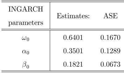
We also apply the P-QMLE in Christou and Fokianos (2014) to the Polio data, giving

the results in Table 5.1a.

INGARCH

parameters Estimates: ASE

!0 0:6401 0:1670

0 0:3501 0:1289

0 0:1821 0:0673

Table 5.1a: P-QML estimates and their asymptotic standard errors for the NB2-INGARCH(1;1)model from the Polio data.

The …tted model is then given by

Xtj Ft 1 P b

p t ;

8 < :

bp_t = 0:6401 + 0:3501Xt 1+ 0:1821b

p

t 1; 2 t 168

bp₁ =X = 1:3333;

with persistence parameter0:5322 and estimated mean 0:6401

1 (0:3501+0:1821) = 1:3683:

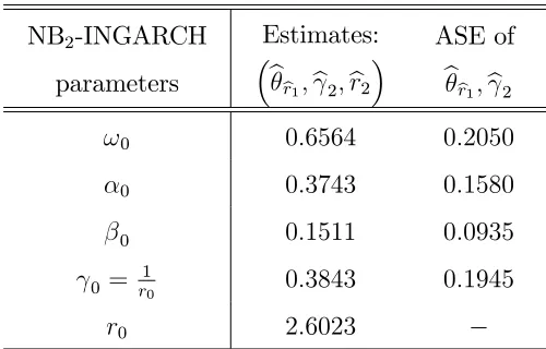
To compare with Zhu’s(2011)…t and the Poisson QMLE of Christou and Fokianos(2014)

we estimated a NB2-INGARCH(1;1) model (4:9) using the 2SNB-QMLE (Algorithm 3.1).

In implementing Algorithm 3.1 we used the same devices as in Section 4.2. More precisely,

the initial dispersion parameter r is calculated using (4:17) giving r = _{3:5050 1}(1:3333)_:33332 =

0:8186while the starting values of the INGARCH(1;1)equation(4:3b)are taken as in(4:16).

The initial conditional mean parameter (0) of the optimization problem (3:3) is obtained

while preliminarily running the Geometric QMLE on the polio series with initial parameter

(2;0:3;0:6)0_{. The estimated parameters of the model and their ASE are summarized in Table}

5.1b. The ASE’s are calculated from the asymptotic distribution of the 2SNB-QMLE given

by Theorem 3.3. In particular, the ASE of_b2 = (_br2) 1 is computed from(3:14b) and (3:16)

while the ASE of br_b2 is obtained from (3:14d) and (3:15). Note that the ASE of br2 is not

available since the asymptotic distribution of_br2 has not a usual form, but may be estimated

using parametric bootstrap.

NB2-INGARCH

parameters

Estimates: b_rb1;_b2;_br2

ASE of b_rb1;_b2

!0 0:6564 0:2050

0 0:3743 0:1580

0 0:1511 0:0935

0 = r10 0:3843 0:1945

r0 2:6023

Table 5.1b: 2SNB-QML estimates and their asymptotic standard errors for the NB2-INGARCH(1;1) model from the Polio data.

The …tted model (4:9)using the 2SNB-QMLE is given by

Xtj Ft 1 N B br2; br2

b

r2+bt ; (5:3)

b

r2 = 2:6023;

8 < :

bt = 0:6564 + 0:3743Xt 1 + 0:1511bt 1; 2 t 168

with persistence parameter 0:3743 + 0:1511 = 0:5254. Note that our estimate of the mean

E(Xt) is _{1 (0:3743+0}0:6564_:1511) = 1:3834; which is closer to the sample meanX = 1:3333 than the

estimated mean, 0:9836, given by Zhu’s (2011) model. However, the estimated mean given

by the P-QMLE is slightly better than the estimated mean given by the2SN B-QM LE. On

the other hand, some properties of the residuals are shown in Figure 5.2a. From the sample

autocorrelation and partial autocorrelation functions in Figure 5.2a (panels(a)and (b)), the

residuals look like a white noise. However, a visual inspection (cf. Figure 5.2a, panels (c)

and (d)) reveals that the normality assumption of the residuals is untenable.

0 2 4 6 8 10 12 14 16 18 20

-0.2 0 0.2 0.4 0.6 0.8 Lag S am pl e A ut oc orr el at ion

Sample Autocorrelation Function of the residual

0 2 4 6 8 10 12 14 16 18 20

-0.2 0 0.2 0.4 0.6 0.8

Sample Partial Autocorrelation Function of the residual

Lag S am pl e P art ial A ut oc orr el at ions

(a) (b)

-10 -5 0 5 10 15

0 0.05 0.1 0.15 0.2 0.25 0.3 0.35 Residuals Dens it y

-3 -2 -1 0 1 2 3

-6 -4 -2 0 2 4 6 8 10 12

Standard Normal Quantiles

Quant il es of I nput S am pl e

QQ Plot ofresiduals versus Standard Normal

(c) (d)

Figure 5.2a: Residual analysis for the Polio series.

(a) Sample autocorrelations of residuals. (b) Sample partial autocorrelations of residuals.

(c)Kernel density of residuals.

(d) QQ-plot of the residuals versus the standard normal distribution.

ran-domized quantile residuals used in Zhu (2011). The residuals are given by _bet = 1(pt);

where 1 _{is the inverse of the standard normal cumulative distribution andp}

t is a random

number uniformly chosen in the interval

h

F Xt 1;bbr;br2 ; F Xt;bbr;rb2

i

;

F x;b_br;br2 being the cumulative function of the NB2 distribution evaluated atxwith

para-metersb_br andbr(cf. Zhu,2011; Benjamin etal,2003). In summary, regarding the stability of

the estimated model, the signi…cance of its coe¢cients and the randomized residual analysis

in Figure 5.2b, it can be concluded that the estimated model is acceptable.

0 2 4 6 8 10 12 14 16 18 20

-0.2 0 0.2 0.4 0.6 0.8

Sample Autocorrelation Function

Lag S am pl e A ut oc orr el at ion

0 2 4 6 8 10 12 14 16 18 20

-0.2 0 0.2 0.4 0.6 0.8

Sample Partial Autocorrelation Function

Lag S am pl e P art ial A ut oc orr el at ions

(a) (b)

-4 -3 -2 -1 0 1 2 3 4

0 0.05 0.1 0.15 0.2 0.25 0.3 0.35 0.4 Randomized residuals Dens it y

-3 -2 -1 0 1 2 3

-4 -3 -2 -1 0 1 2 3

QQ Plot of randomized residuals versus Standard Normal

Standard Normal Quantiles

Quant il es of I nput S am pl e

(c) (d)

Figure 5.2b: Randomized residual analysis for the Polio series. (a) Sample autocorrelations of randomized residuals. (b)Sample partial autocorrelations of randomized residuals.

(c)Kernel density of randomized residuals.

(d) QQ-plot of the randomized residuals versus the standard normal distribution.

Now we compare in-sample performance of our …t (5:1) with that of Zhu (2011) and

Squares (RSS) induced by models (5:1), (5:2) and (5:3). These RSS’s are given respec-tively by RSS bt = P168_t=2 Xt bt

2

, RSS(2_bt) = P168_t=2(Xt 2bt)

2

and RSS bp_t =

P168

t=2 Xt b p t

2

starting from initial valuesb1 =b

p

1 =b1 =X. The latter initial value was

considered by Zhu (2011).

Predictors bt 2bt b p t

RSS 535:1793 540:6634 533:5275

Table 5.2: Residual sum of squares (RSS) of the predictors

b_t (5:2), 2_bt (5:1) and bp_t (5:3)for the Polio series.

From Table 5.2 it can be seen that our model estimated by the 2SNB-QMLE (Algorithm

3.1) outperforms the model of Zhu (2011) with smaller Residual Sum of Squares (RSS).

Since the conditional mean may be in‡uenced by the choice of the initial values, we have

calculated several RSS corresponding to models (5:1), (5:2) and (5:3), starting from several

initial values b1, b

p

1 and b1. The unreported results were virtually the same. However,

the model obtained from the P-QMLE is slightly better than our model with RSS equaling

533:5275.

Finally, Figure 5.3 displays the polio data together with the 2SNB-QML estimated

con-ditional meanbt and the estimated conditional variance given bybvt=bt 1 + _rb1₂bt , where

the conditional overdispersion phenomenon seems reproduced.

19700 1972 1974 1976 1978 1980 1982 1983

5 10 15 20 25

year

Polio series

Estimated conditional mean Estimated conditional variance

5.2. Transaction data

The second dataset is the number of transactions per minute for the stock Ericsson B during

July 05, 2002. This series has a total ofn= 460observations representing the transaction of

approximately 8 hours (from 09:35 through 17:14, cf. Figure 5.4). It was used by Fokianos

et al (2009), Davis and Liu (2016) and Christou and Fokianos (2014) among others. Like the Polio data, the Transaction series is overdispersed in view of its sample mean and sample

variance, which are equal to 9:8239 and 23:7532 respectively. It is characterized by small

values, an asymmetric marginal distribution and a locally constant behavior (cf. Figure 5.4).

0 50 100 150 200 250 300 350 400 450

0 5 10 15 20 25 30 35

Time

Num

ber

of

t

rans

ac

ti

ons

0 5 10 15 20 25 30 35

0 20 40 60 80 100 120 140

Histogram of the Transactions data

(a) (b)

Figure 5.4: Number of transactions per minute for the stock Ericsson B during July 05, 2002. (a) Series. (b) Histogram.

Using the Poisson QMLE, Christou and Fokianos (2014) …tted a NB2-INGARCH(1;1)

model (4:9)to the Transaction data. They found the following speci…cation

Xtj Ft 1 N B br;_br+rb_b

t ; (5:4)

b

r= 7:0220;

8 < :

bt= 0:5808 + 0:1986Xt 1+ 0:7445bt 1; 2 t 460

b1 = 0;

with a strong persistence parameter 0:9431 and an estimated mean _{1 0}0:5808_:9431 = 10:2070.

Motivated by the fact that the 2SNB-QMLE (Algorithm 3.1) is more asymptotically

e¢cient than the P-QMLE in the context of the NB2-INGARCH model (cf. Section 4.1.3),

we applied the former estimate to the Transaction series using the same devices as for

the Polio data. Indeed, from (4:17), the initial dispersion parameter is taken to be r =

(9:8239)2

set according to (4:16). The parameter estimates and their ASE are summarized in Table

5.3.

NB2-INGARCH

parameters

Estimates: b_rb1;_b2;_br2

ASE of b_rb1;_b2

!0 0:7996 0:4034

0 0:7928 0:0650

0 0:1249 0:0340

0 = r10 0:1279 0:0241

r0 7:8199

Table 5.3: 2SNB-QML estimates and their asymptotic standard errors for the NB2-INGARCH(1;1)model from the Transaction data.

Thus our …tted NB2-INGARCH(1;1)model from the Transaction series using the

2SNB-QMLE is given by

Xtj Ft 1 N B br2;_brbr2

2+bt ; (5:5)

b

r2 = 7:8199;

8 < :

b_t = 0:7996 + 0:7928Xt 1 + 0:1249bt 1; 2 t 460

b1 =X = 9:8134;

with a strong persistence parameter, 0:9177, and an estimated mean, 0:7996

1 0:9177 = 9:7157,

which is closer to the sample mean X = 9:8239 than the estimated mean obtained from the

speci…cation of Christou and Fokianos(2014).

Figure 5.5a shows the sample autocorrelation function (panel (a)), the sample partial

autocorrelation function (panel (b)), the Kernel density (panel (c)) and the QQ-plot (panel

a non-Gaussian white noise is strongly tenable.

0 2 4 6 8 10 12 14 16 18 20

-0.2 0 0.2 0.4 0.6 0.8 Lag S am pl e A ut oc orr el at ion

Sample Autocorrelation Function

0 2 4 6 8 10 12 14 16 18 20

-0.2 0 0.2 0.4 0.6 0.8 Lag S am pl e P art ial A ut oc orr el at ions

Sample Partial Autocorrelation Function

(a) (b)

-15 -10 -5 0 5 10 15 20 25 30

0 0.01 0.02 0.03 0.04 0.05 0.06 0.07 0.08 0.09 0.1 Residuals Dens it y

-4 -3 -2 -1 0 1 2 3 4

-15 -10 -5 0 5 10 15 20 25

Standard Normal Quantiles

Quant iles of Input S am pl e

QQ Plot of Sample Data versus Standard Normal

(c) (d)

Figure 5.5a: Residual analysis for the Transaction series.

(a) Sample autocorrelations of residuals. (b) Sample partial autocorrelations

of residuals. (c)Kernel density of residuals. (d) QQ-plot of residuals versus the standard normal distribution.

However, from Figure 5.5b it turns out that the randomized residuals calculated as above

look like a Gaussian white noise regarding the sample autocorrelations and partial

the normal distribution (panel (d)).

0 2 4 6 8 10 12 14 16 18 20

-0.2 0 0.2 0.4 0.6 0.8

Sample Autocorrelation Function

Lag S am pl e A ut oc orr el at ion

0 2 4 6 8 10 12 14 16 18 20

-0.2 0 0.2 0.4 0.6 0.8

Sample Partial Autocorrelation Function

Lag S am pl e P art ial A ut oc orr el at ions

(a) (b)

-6 -4 -2 0 2 4 6

0 0.05 0.1 0.15 0.2 0.25 0.3 0.35 Randomized residuals Dens it y

-4 -3 -2 -1 0 1 2 3 4

-4 -3 -2 -1 0 1 2 3 4 5

Standard Normal Quantiles

Quant iles of I nput S am pl e

QQ Plot of Transaction Data versus Standard Normal

(c) (d)

Figure 5.5b: Randomized residual analysis for the Transaction series.

(a)Sample autocorrelations of randomized residuals. (b)Sample partial

autocorrelations of randomized residuals. (c)Kernel density of randomized residuals.

(d) QQ-plot of the randomized residuals versus the standard normal distribution.

Next we compare the RSS of our …t (5:5) with that of Christou and Fokianos (2014)

given by (5:4). Because of the high persistence parameters in both models, the RSS’s may

be in‡uenced by the starting values for the moderate sample size of the Transaction series.