Munich Personal RePEc Archive
The Choice of Technology and
Rural-Urban Migration in Economic
Development
Zhou, Haiwen
20 October 2017
1
The Choice of Technology and Rural-Urban
Migration in Economic Development
Haiwen Zhou Abstract
This paper studies a general equilibrium model of rural-urban migration in which manufacturing firms engage in oligopolistic competition and choose increasing returns technologies to maximize profits. Urban residents incur commuting costs to work in the Central Business District. Surprisingly a change in the size of the population or an increase in the exogenously given wage rate will not affect a manufacturing firm’s choice of technology. This helps to explain why firms in developing countries may not adopt labor intensive technologies even under abundant labor supply. An increase in the number of manufacturing firms increases both the employment rate and the level of employment in the manufacturing sector. However, manufacturing firms choose less advanced technologies. Capital accumulation leads manufacturing firms to choose more advanced technologies, but may not increase employment in the manufacturing sector.
Keywords: Economic development, the choice of technology, rural-urban migration, increasing returns, urbanization
JEL Classification Numbers: O14, O18, R14
1. Introduction
Economic development is associated with structural changes as labor force relocates from the agricultural sector to the manufacturing sector (Lewis, 1954). With the existence of high levels of fixed costs of production, modern technologies displays significant degrees of increasing returns (Chandler, 1990). Even though advanced technologies have high levels of labor productivity, those technologies with high levels of fixed costs associated with capital equipments may not be the best technologies for a developing country with limited supplies of capital and the choice of appropriate technologies is a long-lasting interesting question in economic development (Sen, 1960, Stewart, 1977). While the classic models of rural-urban migration such as Lewis (1954), Ranis and Fei (1961), and Harris and Todaro (1970) have received a lot of deserved attention, surprisingly, the choice of increasing returns technologies in a general equilibrium model of rural-urban migration has not been addressed formally in the literature.
2
concentrated at the Central Business District (CBD). Following Harris and Todaro (1970), we assume that the wage rate in the manufacturing sector is exogenously given.1 With the rigid
manufacturing wage rate higher than the market clearing wage rate, workers in the manufacturing sector are subject to unemployment/underemployment.
Rural-urban migration is a very significant issue in the process of economic development. Most of the megacities in the world currently are located in developing countries (Todaro and Smith, 2012, chap. 7). Rural-urban migration has led to the existence of a large informal sector in the cities of many developing countries (Rauch, 1993). In this model, individuals consider moving into the manufacturing sector by comparing the wage rate in the agricultural sector and the expected wage rate in the manufacturing sector.
A manufacturing firm’s fixed costs consist of capital only and its marginal costs consist of labor only. The existence of fixed costs of production leads to increasing returns in the manufacturing sector. With increasing returns, the type of market structure in the manufacturing sector is oligopoly. Manufacturing firms choose their levels of output and technologies to maximize profits.
A more advanced technology is specified as a technology with a higher fixed but a lower marginal cost of production. When a manufacturing firm chooses its technology, it faces the following tradeoff. The marginal benefit of adopting a more advanced technology is that marginal cost of production decreases. The higher the level of output, the higher is the saving on total marginal cost. The marginal cost of adopting a more advanced technology is that the fixed costs composed of capital are higher. A manufacturing firm’s optimal choice of technology leads to the equalization of the marginal benefit and marginal cost of adopting a more advanced technology.
With the conditions for the optimal choices of output and technologies established, we then impose various market clearing conditions, including markets for the agricultural good, the manufactured good, labor, and capital. Also, since individuals have equal ownership of land, capital and possible profit, we also impose the condition that the sum of revenue distributed to individuals is equal to the sum of returns to land, capital, and firms.
1 The wage rate is rigid could be a result of government regulations or the existence of unions. Alternatively, the wage
3
We show that when the number of manufacturing firms is exogenously given, an increase in the number of manufacturing firms causes both the employment rate and the level of employment in the manufacturing sector to increase. However, manufacturing firms choose less advanced technologies when the number of firms increases. This result that a decrease in the number of firms induces each firm to adopt more advanced technologies is consistent with the usage of industrial policies in countries such as South Korea to restrict the number of firms in strategic industries (Wade, 1990, Amsden, 2001).
Surprisingly a change in the manufacturing wage rate does not affect the level of manufacturing technology even though this kind of change affects the costs of labor for a manufacturing firm. The reason is as follows. In this general equilibrium model, the equilibrium level of technology may be affected by multiple equilibrium conditions. In addition to the condition for the optimal choice of technology, another condition affecting the equilibrium level of technology is that the quantity supplied and quantity demanded of capital should be equal. First, when the number of manufacturing firms is exogenously given, if the manufacturing wage rate increases, the return to capital will increase correspondingly according to a firm’s condition for the optimal choice of technology. Since the impact of a higher wage rate is cancelled out by the impact of a higher cost of capital, the level of technology in the manufacturing sector does not change with the manufacturing wage rate. In this case, the level of technology is determined by the condition for the clearance of the market for capital. Second, when the number of manufacturing firms is endogenously determined by the zero profit condition, the price and the level of output of a manufacturing firm will change correspondingly if the manufacturing wage rate increases. These changes will cancel out the impact of a change in the manufacturing wage rate. As a result, a firm’s equilibrium choice of technology determined by the condition for the optimal choice of technology and the condition for the clearance of the market for capital is not affected by the level of the manufacturing wage rate.
4
technology. Thus an increase in the size of the population will not affect the equilibrium level of technology in this general equilibrium model. This result that the size of the population may not affect the level of technology helps to explain why firms in developing countries may not adopt labor intensive technologies even under abundant labor supply. In the literature, White (1978) and Pack (1982) have discussed factors preventing firms from choosing appropriate technologies, such as training and information costs. Here we show that firms actually may not adopt labor intensive technologies even without training and information costs.
We show that capital accumulation may not increase the level of employment in the manufacturing sector. The reason behind this is that an increase in the amount of capital leads manufacturing firms to choose more advanced technologies. Because the marginal cost of labor for each unit of output for a more advanced technology decreases, total employment in the manufacturing sector may not increase with capital accumulation. In Lewis (1954), capital accumulation is equivalent to job creation. The Lewis model has been criticized because capital accumulation leads to the adoption of more labor saving technologies while employment in the manufacturing sector may not increase (Todaro and Smith, 2012, p. 118). Here we provide a formal presentation that when manufacturing firms choose among increasing returns technologies, the level of employment in the manufacturing sector may not increase with the endowment of capital.
This paper is related to three lines of literature. First, this paper is related to the literature on rural-urban migration in the process of economic development, such as Harris and Tadaro (1970), Zhang (2002), and Yuki (2007). However, the choice of technologies in the manufacturing sector is not studied in the above models.
Second, this paper is related to the literature studying urban spatial structure, as surveyed in Anas et al. (1998). More specifically, Wheaton (1974) and Takuma and Sasaki (2000) have conducted comparative statics on urban spatial structure. However, rural-urban migration and the choice of technologies in the manufacturing sector are not addressed in this line of literature.
5
adoption of increasing returns technologies when an economy may employ either constant or increasing returns technologies to produce a manufactured good.2 While Murphy et al. (1989)
have focused on a closed economy, Trindade (2005) also considers the impact of international trade on the adoption of increasing returns technologies. Different from the literature on the choice of technology in the 1960s and 1970s which mainly focused on the possibilities of more job creation by adopting more labor intensive technologies, the possibility of the existence of multiple equilibria is the main concern in Murphy et al. (1989) and Trindade (2005). Rural-urban migration and the urban spatial structure are not addressed in the above models.
The plan of the paper is as follows. Section 2 specifies the model. Section 3 studies the equilibrium in which the number of manufacturing firms is exogenously given. Section 4 revisits the equilibrium in which the number of manufacturing firms is endogenously determined by the zero-profit condition. Section 5 discusses some possible generalizations and extensions of the model and concludes.
2. Specification of the model
In this economy, there are three factors of production: labor, capital, and land. The size of the population is L and each individual is endowed with one unit of labor. The endowment of capital is K. The total amount of land in this economy is T. All individuals are assumed to have the same preferences. An individual derives utility from the consumption of three types of goods: an agricultural good, a manufactured good, and residential land. First, the agricultural good is produced by labor and land with a technology exhibiting constant returns. The number of individuals working in the agricultural sector is La. Second, the manufactured good is produced by labor and capital. The number of individuals working in the manufacturing sector is Lm. Third, land may be used for residence directly.
We assume that the production of the agricultural good does not need to be concentrated. Agriculture is located in rural areas. Rural land is used both for residential purposes and for the production of the agricultural good. Regardless of the usage, land in the agricultural sector has the same level of rent. The manufacturing sector is located in the urban area. Urban land is used for
2 There are several significant differences between this model and Murphy et al. (1989). First, capital is not a factor
6
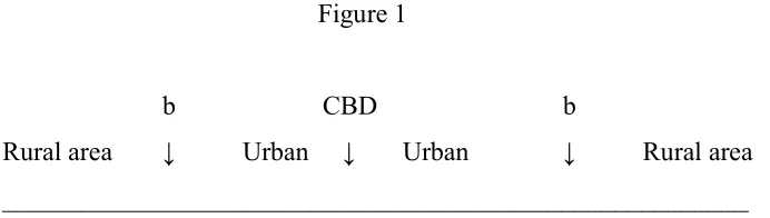
[image:7.612.143.489.156.254.2]residential purposes only. Depending on the distance from the CBD, land at different locations in the urban sector may have different levels of rents. The spatial structure of this economy is specified as a linear city type as shown in Figure 1.
Figure 1
b CBD b
Rural area ↓ Urban ↓ Urban ↓ Rural area
________________________________________________________
In Figure 1, the total length of the line is T and the center of this line is the CBD. Similar to the urban economics literature, we assume that the production of the manufacturing good needs to be concentrated in the CBD.3 Workers employed in the manufacturing sector live on the two
sides of the CBD and workers employed in the agricultural sector live in the rural areas which are located relatively far away from the CBD. The points b (determined endogenously in equilibrium) are the division points of the rural areas and the urban sector. The higher the number of workers employed in the manufacturing sector, the higher the demand for residential land in the urban sector, and the larger the distance between the CBD and the two points b. Workers employed in the manufacturing sector need to commute to the CBD to work. Commuting takes time only, and no pecuniary cost is involved. Except for commuting costs, there is no transportation cost for the agricultural good and the manufactured good. Workers employed in the manufacturing sector choose where to live. Rents in the urban sector are bid up in such a way that utilities at different locations will be the same: a location closer to the CBD has a lower commuting cost but a higher level of rent.
Let ca denote a representative consumer’s consumption of the agricultural good, cm denote her consumption of the manufactured good, and q denote her consumption of residential land. For (0,1), this representative consumer’s utility function is specified as
q c c q c c
U( a, m, ) a m1 . (1)
3 One justification of this assumption that manufacturing firms need to be concentrated in the CBD is that
7
Residents have an equal share of land, capital, and firms. A consumer’s total income I is the sum of the wage income and ownership from land, capital, and firms. The exogenously given wage rate at the CBD is w. If there are no commuting costs, an individual is able to supply one unit of labor. The per unit commuting cost in terms of the amount of labor used is . For a worker employed in the manufacturing sector with a distance s from the CBD, the amount of time spent on commuting is s. This person is able to supply 1s units of labor to a manufacturing firm. The employment rate in the urban sector is e. Rather than interpreting e as the percentage of workers employed in the manufacturing sector, in this model it is interpreted as the percentage of time that an individual in the manufacturing sector is employed.4 Since the probability of being
employed is e, the expected wage income of an individual employed in the manufacturing sector is (1s)ew.
The per capita income from ownership of land, capital, and firms is . An individual commuting a distance of s with income from ownership of land, capital, and firms of has a total income of (1 s)ew :
s ew
I (1 ) . (2)
The price of the agricultural goods is pa and the price of the manufactured good is pm. Similar to Takuma and Sasaki (2000), a consumer’s consumption of residential land is exogenously fixed at q. Since all individuals have the same level of utility in equilibrium, without loss of generality, we focus on the study of an individual located at one of the two points b. Let
the rent at the border of the rural area and the urban sector be r(b). This consumer’s total spending on the three types of goods is paca pmcm r(b)q. This consumer’s budget constraint states that
I q b r c p c
pa a m m ( ) . (3)
A consumer chooses the quantities of consumption of the agricultural good and the manufactured good to maximize utility (1), subject to her budget constraint (3). For an individual living closer to the CBD, the increased wage income is exactly offset by the higher level of rent. As a result, individuals reach the same level of utility in equilibrium. For a consumer located at
4 One advantage of this interpretation is that every individual in the manufacturing sector has a positive income and
8
one of the borders of the rural areas and the urban sector, this consumer’s utility maximization leads to the following levels of demand for the agricultural good and the manufactured good:
a
a I pr b q
c ( ) , (4)
m
m pI r b q
c (1) ( ) . (5)
For the production of the manufactured good, both capital and labor are needed: capital is the fixed cost and labor is the marginal cost of production. The existence of fixed costs of production leads to increasing returns in the manufacturing sector. Similar to Zhou (2004, 2007, 2009), to produce the manufactured good, we assume that there is a continuum of increasing returns technologies indexed by a positive number n.5 A higher value of n indicates a more
advanced technology. The fixed cost associated with technology n in terms of the amount of capital used is f(n) and the marginal cost in terms of the amount of labor used is (n). To capture the substitution between fixed and marginal costs of production, we assume that the fixed cost increases while the marginal cost decreases with the level of technology: f ('n)0 and
0 ) ('n
.6 We also assume that f' ('n)0 and ' ('n)0. That is, when a more advanced
technology is chosen, the fixed cost increases at a nondecreasing rate and the marginal cost decreases at a nonincreasing rate.
The number of identical firms producing the manufactured good is m. Firms producing the manufactured good are assumed to engage in Cournot competition. They choose their levels of output and technologies to maximize profits. The per unit cost of capital is R . For a manufacturing firm with output level x, the revenue is pmx and the costs of capital are f R and
the costs of labor are xw. Thus its profit is pmx f Rxw. A manufacturing firm’s optimal
5 Zhou (2009) provides a more detailed illustration of the adoption of increasing returns technologies in the process
of economic development for firms engaging in oligopolistic competition.
6 The adoption of containers in the transportation sector illustrates the substitution between fixed and marginal costs
9
choice of output requires that 0
w
x p x
p m
m . With the specification of the utility function
in equation (1), the absolute value of a consumer’s elasticity of demand for the manufactured good is one. Plugging this result into the condition for a manufacturing firm’s optimal choice of output leads to
w m
pm
1 1 . (6)
A manufacturing firm’s optimal choice of technology leads to7
0 )
(' )
('
f n R n xw . (7)
From equation (7), a manufacturing firm’s choice of technology n could be affected by the endogenous variables R and x, and the exogenous parameter w. As will be shown later on, since the endogenous variables R and x could be affected by the exogenous parameter w , in equilibrium, a firm’s choice of technology may not be affected by the manufacturing wage rate w
.
For the labor market in the manufacturing sector, an individual living in the CBD does not incur any commuting cost. There are Lm/2 individuals employed on each side of the CBD. Since each of the Lm/2 individuals need q units of land for residence, an individual living in the border
of the rural sector and the urban sector needs to travel a distance of qLm/2 and has commuting
costs of qLm/2. Thus the average amount of commuting time for a urban resident is qLm /4
and the total commuting time of the Lm individuals in the urban sector is qLm2 /4. Deducting the level of commuting time, the total amount of labor available from the Lm individuals employed
in the manufacturing sector is 2
4 m
m qL
L . Since the employment rate in the manufacturing
sector is e, the actual provision of labor in the manufacturing sector is
2
4 m
m qL
L
e . Each of
the m manufacturing firms demands x units of labor and the total demand for labor in the
7A second order condition corresponding to (7) is f ''R ''xw0. With the assumptions on fixed and marginal
10
manufacturing sector is mx. Equilibrium of the labor market in the manufacturing sector requires that
2
4 m
m qL
L e x
m . (8)
For the labor market for this economy as a whole, demand for labor is the sum of demand from the manufacturing sector and the agricultural sector. Employment in the manufacturing sector is Lm and employment in the agricultural sector is La. Thus total demand for labor in this economy is La Lm. Total supply of labor is L. The clearance of the labor market for this economy requires that
L L
La m . (9)
For the market for capital, each of the m manufacturing firms demands f units of capital and the total demand for capital is m f . Total supply of capital is K. The clearance of the market for capital requires that
K f
m . (10)
For the market for the agricultural good, from equation (4), each of the L consumers demands
I r(b)q
/ pa units of the agricultural good and the total demand for the agriculturalgood is L
I r(b)q
/ pa. Since each of the L individuals needs q units of land for residence,the total amount of land used for residence is qL. Thus the remaining amount of land available for the production of the agricultural good is T qL. For (0,1), the level of output of the agricultural good is specified as L 1 (T qL)
a . That is, total supply of the agricultural good is
( )
1 T qL
La . The clearance of the market for the agricultural good requires that
a
p q b r I
L ( ) L 1 (T qL)
a . (11)
For the market for the manufactured good, from equation (5), each of the L consumers demands (1)
Ir(b)q
/ pm units of the manufactured good and total demand for themanufactured good is L(1)
Ir(b)q
/ pm. Each of the m manufacturing firms supplies x11
m
p
q b r I L(1) ( )
x m
. (12)
The amount of rents for a location in the urban sector with a distance of s from the CBD is determined by the condition that individuals living at different locations of the urban sector have the same level of utility. Deducting the amount of income spent on paying rents, an individual living at any location has the same amount of income (1s)ewr(s)q, which is spent on the agricultural good and the manufactured good. That is, (1s)ewr(s)q paca pmcm . Rearrangement of this equation leads to
q c p c p w
e s s
r( )[(1 ) a a m m]/ . (13)
For land on the borders of the rural sector and the urban sector (points b), it may be used either for residential purposes or for the production of the agricultural good. If it is used for residential purposes, the return is r(b). If it is used for the production of the agricultural good, the return is the marginal value product of land p L 1(T qL)1
a
a . In equilibrium, the returns to
land on points b used for either residential or agricultural purposes should be equal: 1
1 ( )
)
(
L q T L p b
r a a . (14)
Urbanization rates in developing countries are higher than those in developed countries when they were at similar levels of income (Todaro and Smith, 2012, chap. 7). In this model, a worker may be employed either in the agricultural sector or move to the manufacturing sector. Individuals consider whether to move into the manufacturing sector or not by comparing the wage rate in the agricultural sector and the expected wage rate in the manufacturing sector. A worker employed in the agricultural sector lives close to his work place and does not incur any commuting costs. This worker is paid by the marginal value product of labor in the agricultural sector, which is (1 )p L (T qL)
a
a
. A worker’s expected return in the manufacturing sector is
w e L q m
2
1 . For a worker to be indifferent between employed in the agricultural sector and
employed in the manufacturing sector, the return in the two sectors should be equal:
w e L q L
q T L
pa a m
2 1 ) (
) 1
12
To complete the model, we need to determine the profit of a manufacturing firm. Depending on whether the entry into the manufacturing sector is blocked or free, a manufacturing firm’s profit may be positive or zero. In the following, we study the two scenarios in turn.
3. The equilibrium with an exogenous number of firms in the manufacturing sector
Before the 1980s, many developing countries adopted the import substitution strategy to develop their manufacturing sector. To support domestic firms, tariffs and quotas were frequently used to limit international competition. Countries such as South Korea used licenses to limit the number of firms in strategic industries (Cimoli et al., 2009). Patents could also make entry of new domestic firms in the manufacturing sector unlikely. In this section, we study the equilibrium in which the number of manufacturing firms is exogenously given. With blocked entry, the profit of a manufacturing firm will be nonnegative.
Each unit of land in this economy earns a level of rent not lower than that of the agricultural sector, which is equal to r(b). Land in the urban sector earns extra rents. The total amount of extra rents in the urban sector is equal to the total commuting costs of urban residents 2/4
m
L q w e
. Thus the total amount of rents in the economy is 2
4 )
(b ewqLm
r
T . This amount of total rents
2 4
)
(b ewqLm
r
T , profits from the manufacturing sector n , and the total return to capital RK
are shared equally by all L individuals. Remember that pmx f Rxw. Thus the total
amount of revenue from ownership of land, capital, and firms is
RK w x R f x p m L q w e b r
T ( )4 m2 ( m )
. Each of the L individuals receives and the
total amount of revenue from ownership of land, capital, and firms is L. In equilibrium, we have
L RK w x R f x p m L q w e b r
T m m
( )
4 )
( 2 . (16)
Plugging the value of r(b) from equation (14) into equation (16) leads to
p L T qL
ewqL m p x f R xw RK LT a a m m
( )
4 )
( 1 2
1 . (17)
13 m
p , R, x, n, La, Lm, I, , r, and e as functions of exogenous parameters. An equilibrium when the number of firms is exogenously given is a tuple ( pa, pm, R, x, n, La, Lm, I, , r,
e) satisfying equations (2), (6)-(12), (14), (15), and (17).8 For the rest of the paper, we use the
price of the agricultural good as the numeraire: pa 1.
To conduct comparative statics, we need to reduce the system of eleven equations to a smaller and thus manageable number of equations. Simplification of the above system of eleven equations leads to the following system of three equations defining three endogenous variables Lm , e, and n as functions of exogenous parameters:9
0 ) ( ) ( ) 1 ( 2 1
1
m
m ew TL qLL
L
q , (18a)
04 ) )( 1 ( 1
1 1 2
2
m m
m T qL ew L qL
L L m
, (18b)0
3
m f K . (18c)
Partial differentiation of the system of equations 1, 2, and 3 with respect to e, La,
n, w, L, T , m, K , and
leads todL L L w d w w dn dL de n L e L e m m m 0 0 0 0 0 0 2 1 2 1 3 2 2 1 1
8 For this system of equations (2), (6)-(12), (14), (15), and (17) defining the equilibrium in which the number of
manufacturing firms is exogenously given, if equations (2), (6)-(12), (14), and (15) are satisfied, it can be checked that equation (17) is always satisfied. That is, one equation is redundant. With Walras’s law in mind, this redundancy is not surprising.
9Equations (18a)-(18c) are derived as follows. First, equation (18a) is derived by plugging the value of
14 d dK K dm m m dT T T 0 0 0 0 0 2 1 3 3 2 2 1
. (19)
Let denote the determinant of the coefficient matrix of (19):
e L L e
n3 1 m2 m1 2 . Partial differentiation of equations (18a)-(18c) leads to
0 1
e , 0
1
m
L , 2 0
m
L , 2 0
e , and 3 0
n . As a result, 0. With nonsingular,
there exists a unique equilibrium for the system (19).
When the manufacturing wage rate increases, labor costs for a manufacturing firm increase. Will this lead a manufacturing firm to choose a more advanced technology to decrease the usage of labor? When the manufacturing wage rate increases, will more workers enter into the manufacturing sector? The following proposition studying the impact of a change in the manufacturing wage rate will answer those questions.
Proposition 1: An increase in the manufacturing wage rate decreases the employment rate in the manufacturing sector, and does not change the level of employment and the level of technology in the manufacturing sector.10
Proof: An application of Cramer’s rule on the system (19) leads to
0 / 2 1 2 1
3
m
m w w L
L n w d
de ,
3 1 2 1 2 /
w e e w n w d
dLm , and 0
w d
dn .
Partial differentiation of equations (18a) and (18b) leads to 1 2 1 2 0
w e e
w . As a result,
0
w d
dLm .
10 Similar to the proof of Proposition 1, it can be shown that when the number of manufacturing firms is exogenously
15
To understand Proposition 1, when the manufacturing wage rate increases, the expected wage rate does not change because the employment rate decreases correspondingly. As a result, the level of employment in the manufacturing sector does not change. As discussed in the Introduction, when the manufacturing wage rate increases, the cost of capital R increases correspondingly so that the condition for a manufacturing firm’s optimal choice of technology (equation (7)) is always satisfied. That is, when x and w change, R will change correspondingly so that equation (7) remains valid. Since the impact of an increase in the wage rate is cancelled out by the impact of an increase in the cost of capital, the level of technology in the manufacturing sector does not change with the manufacturing wage rate. Instead, the level of technology is determined by the condition for the clearance of the market for capital (equation (10)).
An increase in the size of the population increases the supply of workers. Will this decrease the cost of labor and lead manufacturing firms to choose less advanced technologies using more labor? Will this decrease the employment rate in the manufacturing sector? The following proposition studying the impact of a change in the size of the population does not give an unambiguous answer on the level of employment in the manufacturing sector.
Proposition 2: When the size of the population increases, the level of technology of a manufacturing firm does not change, and the impact on the level of employment and employment rate in the manufacturing sector is ambiguous.
Proof: An application of Cramer’s rule on (19) leads to
3 1 2 1 2 /
m
m L L L
L n dL
de , 3 1 2 1 2 /0
L e e L n dL
dLm , and 0
dL dn
. Partial differentiation of equations (18a) and (18b) leads to 1/Lm 0, , 1/L0, and 0
/
2
Lm . Because the sign of 2 /L is ambiguous, the signs of de/dL and dLm/dL are
ambiguous.
16
land available for the production of the agricultural good. Thus the value marginal product of an individual employed in the agricultural sector decreases. Through the labor market equilibrium condition, this effect decreases the employment rate in the manufacturing sector. Second, an increase in the size of the population increases the demand for the manufactured good. This latter effect increases the employment rate in the manufacturing sector. Without adding more structure to the model, it is not clear which effect dominates and thus the impact of an increase in the size of the population is ambiguous.
Land is used for both residential purposes and for the production of the agricultural good. How will an increase in the amount of land affect the levels of employment and technology in the manufacturing sector?
Proposition 3: An increase in the amount of land increases the employment rate, and does not change the level of employment in the manufacturing sector and the level of technology of a manufacturing firm.
Proof: An application of Cramer’s rule on the system (19) leads to
0 /
2 1 2 1
3
m
m T T L
L n dT
de ,
3 1 2 1 2 /
T e e T n dT
dLm , and
0
dT
dn . Partial differentiation of equations (18a) and (18b) leads to 1 2 1 2 0
T e e
T .
As a result, 0
dT dLm .
17
each other. As a result, the number of individuals employed in the agricultural sector does not change with the endowment of land. An increase in the endowment of land increases the marginal productivity of an individual employed in the agricultural sector. Since the price of the agricultural good is normalized to one, the return to labor in the agricultural sector increases. To maintain equilibrium in the labor market, the employment rate in the manufacturing sector increases. Similar to the discussion of Proposition 1, the return to capital adjusts in such a way that the level of technology in the manufacturing sector does not change with the amount of land.
For a country’s development, the process of industrialization is also the process of urbanization. On the one hand, a country’s level of industrialization has an important impact on this country’s level of urbanization. On the other hand, urbanization is not totally determined by the level of industrialization of a country. For example, it is argued that in Mexico the process of urbanization moved ahead of the process of industrialization (Gilbert and Gugler, 1992). However, in the case of China, it is frequently argued that the process of urbanization has been lagging behind the level of industrialization (Deng et al., 2008). In this model, a change in the level of commuting costs affects the urban spatial structure. Will a change in commuting costs also affect the process of industrialization as measured by the level of employment in the manufacturing sector? The following proposition studies how a change in commuting costs affects the levels of technology and employment of the manufacturing sector.
Proposition 4: An increase in the level of commuting costs increases the employment rate and does not change the level of technology in the manufacturing sector. The impact on the level of employment in the manufacturing sector is ambiguous.
Proof: An application of Cramer’s rule on (19) leads to
0 / 2 1 2 1
3
m
m L
L n d
de
,
3 1 2 1 2 /
n e e
d
dLm , 0
d
dn .
Since the sign of
1 2 1 2 e
e is undetermined, the sign of dLm/d is undetermined.
18
of labor in the manufacturing sector. To maintain labor market equilibrium in the manufacturing sector, the level of employment in the manufacturing sector should increase. Second, an increase in commuting costs decreases the return to an individual employed in the manufacturing sector. As a result, individuals will move out of the manufacturing sector and the level of employment in the manufacturing sector will decrease. Since it is not clear which effect will dominate, the impact of an increase in commuting costs on the level of employment in the manufacturing sector is ambiguous.
Unemployment is a chronic problem for developing countries. Why did not firms in developing countries create enough jobs? While both advanced technologies and higher employment in the manufacturing sector could be desirable for a developing country, the following proposition studying the impact of a change in the degree of competition on the level of employment and technology in the manufacturing sector shows that opposite implications on the level of technology and the level of employment can happen when the number of firms in the manufacturing sector increases.
Proposition 5: When the number of manufacturing firms increases, the employment rate in the manufacturing sector increases, the level of employment in the manufacturing sector increases, and a manufacturing firm chooses a less advanced technology.
Proof: Partial differentiation of equations (18a)-(18c) yields 1 /Lm 0, 1/e0, 0
/
2
m , 2 /e0, 2 /Lm 0, 3 /m0, and 3 /n0. An application of
Cramer’s rule on (19) leads to 1 2 3 /0
n m L dm
de
m
, 1 2 3 /0
n m e dm
dLm , and
0 / 2 1 2 1
3
m
m e e L
L m dm
dn .
19
sector, marginal productivity of an agricultural work increases. To ensure that an individual is still indifferent between working in the agricultural sector and the manufacturing sector, the employment rate in the manufacturing sector increases. When the number of manufacturing firm increases, each firm receives a smaller amount of capital. As a result, each firm chooses a less advanced technology.
In the model of Lewis (1954), capital accumulation leads to the expansion of production and an increase in the level of employment in the manufacturing sector. The following proposition shows that capital accumulation may not necessarily lead to an increase in the level of employment in the manufacturing sector.
Proposition 6: An increase in the amount of capital does not change the employment rate and the level of employment in the manufactured sector. An increase in the amount of capital leads a manufacturing firm to choose a more advanced technology.
Proof: An application of Cramer’s rule on (19) leads to 0
dK
de , 0 dK
dLm , and
0 / 2 1 2 1
3
m
m e e L
L K dK
dn .
To understand Proposition 6, since the number of manufacturing firms is exogenously given, an increase in the amount of capital means that each manufacturing firm receives a higher amount of capital and thus the equilibrium level of technology increases. From equation (8), the level of employment in the manufacturing sector is affected by the number of manufacturing firms, marginal cost in terms of labor units, and output. When the amount of capital in this economy increases, a manufacturing firm chooses a more advanced technology and marginal cost in terms of labor units decreases. However, because the increase in output exactly cancels out the impact of the decrease in the marginal cost, the level of employment in the manufacturing sector does not change.
4. The equilibrium with an endogenous number of firms in the manufacturing sector
20
patents may expire and new firms may enter an industry. In this section, we study the equilibrium in which the number of manufacturing firms is endogenously determined by the zero profit condition.11
With free entry and exit in the manufacturing sector, a manufacturing firm earns a profit of zero:12
0
f R xw x
pm . (20)
With profits from the manufacturing sector equal to zero, the total revenue of the
government is the sum of the total amount of rents 2
4 )
(b ewqLm
r
T and total return to capital
K
R . Each of the L individuals receives a revenue from ownership of land, capital, and firms of and the total amount of revenue received by all individuals from ownership of land, capital, and firms is L. In equilibrium, we have
L K R L q w e b r
T m
2
4 )
( . (21)
Plugging the value of r(b) from equation (14) into equation (21) leads to
p L T qL
ewqL RK LT a a m
1 1 2
4 )
( . (22)
When the number of manufacturing firms is endogenously determined by the zero profit condition, equations (2), (6)-(12), (14), and (15) are still valid. Equations (2), (6)-(12), (14)-(15), (20), and (22) form a system of twelve equations defining a system of twelve variables pa, pm,
R, x, m , La, Lm, I, n, , r, and e as functions of exogenous parameters. An equilibrium in which the number of manufacturing firms is endogenously determined is a tuple (pa, pm, R, x,
m , La, Lm, I, n, , r, e) satisfying equations (2), (6)-(12), (14)-(15), (20), and (22).13
11 See Chao and Yu (1997), Lahiri and Ono (2004), Zhang (2007), and Chen and Shieh (2011) for examples of
oligopolistic competition with free entry.
12 To facilitate presentation, the number of manufacturing firms is specified as a real number, rather than restricted to
be an integer number.
13 For this system of equations (2), (6)-(12), (14)-(15), (20), and (22) defining the equilibrium in which the number of
21
To conduct comparative statics, simplification of this system of twelve equations (2), (6)-(12), (15), (20), and (22) leads to the following system of three equations defining three endogenous variables e, Lm, and n as functions of exogenous parameters:14
0 ) ( ) ( ) 1 ( 2 1
1
m
m ew TL qLL
L
q , (23a)
04 )
)( 1 (
1 1 2
2
m m
m T qL ew L qL
L L K
f
, (23b)
0 ) ('
'
3
f K f . (23c)
Partial differentiation of the system of equations 1-3 with respect to e, Lm, n, w, L, , T, K , and
leads todL L L w d w w dn dL de n n L e L e m m m 0 0 0 0 0 2 1 2 1 3 2 2 2 1 1
dK d
K K dT T T d 0 0 0 0 0 2 1 3 2 2 1
2 . (24)
Let denote the determinant of the coefficient matrix of (24):
e L L e
n3 1 m2 m1 2 . Partial differentiation of equations (23a)-(23c) leads to
0 1
e , 0
1
m
L , 2 0
m
L , and 2 0
e . Partial differentiation of equations (23c) leads to
14Equations (23a)-(23c) are derived as follows. First, equation (23a) is the same as equation (18a). Second, equation
(23b) is derived by plugging the value of m from equation (10) into equation (18b). Third, from equation (20), the level of output of a manufacturing firm can be expressed as x fR/(pmw). Plugging this value of x into
equation (7) leads to f ('pmw)'wf 0. Plugging the value of pm from equation (6) and the value of m
22
0 ) (' ' ''
3
f K f
n
. As a result, 0. With nonsingular, there exists a uniqueequilibrium for the system (24).
The following proposition revisits the impact of a change in the endowment of capital on a manufacturing firm’s choice of technology when the number of manufacturing firms is endogenously determined.
Proposition 7: When the number of manufacturing firms is endogenously determined by the zero-profit condition, an increase in the amount of capital leads a manufacturing firm to choose a more advanced technology.
Proof: An application of Cramer’s rule on (24) leads to
0 /
2 1 2 1
3
m
m e e L
L K dK
dn .
When the number of manufacturing firms is endogenously determined, the impact of an increase in the amount of capital on the employment rate and the level of employment in the manufacturing sector is ambiguous. The reason is as follows. When the amount of capital increases, there are two effects on the level of employment in the manufacturing sector. First, to produce a given level of output, because a manufacturing firm chooses a more advanced technology and the unit labor requirement for each unit of output decreases, the demand for labor in the manufacturing sector decreases. Second, an increase in the amount of capital is an increase in a factor of production and this will lead to an increase in the level of output because capital is fully employed. To produce a higher level of output, the demand for labor in the manufacturing sector increases. Because the two effects work in opposite directions and it is not clear which effect dominates, the impact of an increase in the amount of capital on the level of employment in the manufacturing sector is ambiguous.
23
regardless of whether the number of firms in the manufacturing sector is exogenously given or endogenously determined by the zero-profit condition.
When the number of manufacturing firms is endogenously determined, the reason that an increase in the manufacturing wage rate does not change the level of technology is as follows. From equation (20), a manufacturing firm’s level of output is x f R/(pm
w). Plugging thislevel of output into the condition for a firm’s optimal choice of technology (equation (7)) leads to
0 '
) (
'R p w Rwf
f m
. As a result, R cancels out and the equation reduces to0 '
)
('p w wf
f m
. From equation (6), pm wmm1. From equation (10), m K/ f .Plugging the values of pm and m into f ('pm
w)
'wf 0 leads to0 '
/ 1
1
'
f K wf
w
f
. Simplification of this equation leads to equation (23c) determiningthe level of technology in which the level of the exogenously given wage rate is now absent because a change in the price of the manufactured good cancels out a change in the manufacturing wage rate. That is, as discussed in the Introduction, when the manufacturing wage rate increases, the price of the manufactured good as a markup over the marginal cost increases. The level of output of a manufacturing firm is affected by the price of the manufactured good. Since the output change of a manufacturing firm incorporates the impact of a change in the price of the manufactured good, these changes will cancel out the impact of a change in the manufacturing wage rate. Thus, a manufacturing firm’s choice of technology in equilibrium is not affected by the level of the manufacturing wage rate.
5. Conclusion
24
affects neither the level of employment nor the level of technology in the manufacturing sector. Third, an increase in the size of the population increases the level of employment in the manufacturing sector, and does not change the level of technology of a manufacturing firm. The impact of a change in the size of the population on the employment rate in the manufacturing sector is ambiguous. Fourth, an increase in the amount of land increases the employment rate, and affects neither the level of employment nor the level of technology in the manufacturing sector. Finally, an increase in commuting costs increases the employment rate, and does not change the level of technology in the manufacturing sector.
We have made various assumptions to simplify the analysis. There are some interesting generalizations and extensions of the model. First, in this model with a homothetic preference of consumers, a consumer spends a fixed percentage of income on each type of goods. The incorporation of a non-homothetic preference will lead to more complicated interactions between the agricultural sector and the manufacturing sector. Second, in this model, labor mobility from the rural sector to the urban sector is assumed to be free. In China, labor mobility between rural areas and cities is frequently restricted. Policy analysis such as policies limiting labor mobility between rural areas and cities should be an interesting avenue for future research.
Acknowledgements:
25
References
Amsden, Alice. 2001. The Rise of “The Rest”: Challenges to the West from Late-Industrializing Economies. New York: Oxford University Press.
Anas, Alex, Richard Arnott, and Kenneth Small. 1998. Urban spatial structure. Journal of Economic Literature 34, 1426-1464.
Chandler, Alfred. 1990. Scale and Scope: The Dynamics of Industrial Capitalism. Cambridge, MA: Harvard University Press.
Chao, Chi-Chur, and Eden Yu. 1997. Trade liberalization in oligopolistic competition with unemployment: a general equilibrium analysis. Canadian Journal of Economics 30, 479-496.
Chen, Ming Chieh, and Yeung-Nan Shieh. 2011. Specific commodity taxes, output and location decision under free entry oligopoly. Annals of Regional Science 47, 25-36.
Cimoli, Mario, Giovanni Dosi, and Joseph Stiglitz. 2009. Industrial Policy and Development: The Political Economy of Capabilities Accumulation. New York: Oxford University Press.
Deng, Xiangzheng, Jikun Huang, Scott Rozelle, and Emi Uchida. 2008. Growth, population and industrialization, and urban land expansion of China. Journal of Urban Economics 63, 96-115.
Fei, John, and Gustav Ranis. 1961. A theory of economic development. American Economic Review 51, 533-565.
Gilbert, Alan, and Josef Gugler. 1992. Cities, Poverty, and Development: Urbanization in the Third World. 2nd edition, New York: Oxford University Press.
26
Lahiri, Sajal, and Yoshiyasu Ono. 2004. Trade and Industrial Policy under International Oligopoly. Cambridge, UK: Cambridge University Press.
Levinson, Marc. 2006. The Box: How the Shipping Container Made the World Smaller and the
World Economy Bigger. Princeton, NJ: Princeton University Press.
Lewis, W. Arthur. 1954. Economic development with unlimited supply of labor. Manchester School of Economic and Social Studies 22, 139-191.
Murphy, Kevin, Andrei Shleifer, and Robert Vishny. 1989. Industrialization and the big push.
Journal of Political Economy 97, 1003-1026.
Pack, Howard. 1982. Aggregate implications of factor substitution in industrial processes. Journal of Development Economics 11, 1-37.
Prendergast, Renee. 1990. Scale of production and choice of technique in the engineering industries in developing countries. Journal of Development Studies 27, 72-88.
Rauch, James. 1993. Economic development, urban underemployment, and income inequality.
Canadian Journal of Economics 26, 901-918.
Sen, A. K. 1960. Choice of Techniques. Oxford, UK: Basic Blackwell.
Stewart, Frances. 1977. Technology and Underdevelopment. Boulder, CO: Westview Press.
Takuma, Fumio, and Komei Sasaki. 2000. Spatial structure of a metropolitan area with an agricultural hinterland. Journal of Urban Economics 48, 307-320.
Todaro, Michael, and Stephen Smith. 2012. Economic Development. 11th edition, Boston, MA:
27
Trindade, Vitor. 2005. The big push, industrialization, and international trade: the role of exports.
Journal of Development Economics 78, 22-48.
Wade, Robert. 1990. Governing the Market: Economic Theory and the Role of Government in East Asian Industrialization. Princeton, NJ: Princeton University Press.
Wheaton, William. 1974. A comparative static analysis of urban spatial structure. Journal of Economic Theory 9, 223-237.
White, Lawrence. 1978. The evidence of appropriate factor proportions for manufacturing in less developed countries: a survey. Economic Development and Cultural Change 27, 27-59.
Yuki, Kazuhiro. 2007. Urbanization, informal sector, and economic development. Journal of Development Economics 84, 76-103.
Zhang, Jie. 2002. Urbanization, population transition, and growth. Oxford Economic Papers 54, 94-117.
Zhang, Junxi. 2007. Endogenous markups, intensity of competition, and persistence of business cycles. Southern Economic Journal 74, 546-565.
Zhang, Xiaobo, Jin Yang, and Shenglin Wang. 2011. China has reached the Lewis turning point.
China Economic Review 22, 542-554.
Zhou, Haiwen. 2004. The division of labor and the extent of the market. Economic Theory 24, 195-209.
Zhou, Haiwen. 2007. Factor endowment, the choice of technology, and the volume of trade.
International Economic Journal 21, 593-611.