Characterization of Velocity Pro
fi
le of Highly-Filled GFRP-BMC
through Rectangular Duct-Shaped Specimen during Injection Molding
from SEM Fiber Orientation Mapping
Michael C. Faudree
1, Yoshitake Nishi
2and Michael Gruskiewicz
31Center of Foreign Language, Tokai University, Hiratsuka 259-1292, Japan
2Doctoral Graduate School of Science and Technology, Tokai University, Hiratsuka 259-1292, Japan
3Premix, Inc., North Kingsville, Ohio, 44068, USA
There is an extensive body of research and texts on numerical simulation to obtain rheological properties of injection molded resins and composites, however to our knowledge there is no or little research on estimating velocity profile fromfiber orientation mapping of GFRP-BMCs (glassfiber reinforced polymer bulk molding compounds). This study reports a simple analysis of specific laminar creepflow properties of highly-filled short-fiber GFRP-BMC through a dogbone specimen as a rectangular duct during injection molding from SEMfiber orientation mapping which is found to exhibit a 3-layer [skin-core-skin] structure resembling classical laminarflow through a conduit. Therefore, to characterize the BMC with extremely low Reynolds number³2©10¹4, velocity profile, primary and secondary boundary layers were estimated
from Hermansfiber orientation parameter across gauge section thickness. [doi:10.2320/matertrans.M2013143]
(Received April 15, 2013; Accepted July 4, 2013; Published August 30, 2013)
Keywords: GFRP (Glassfiber reinforced polymers), BMC (Bulk molding compounds), injection molding,fiber orientation, moldflow, rheology, Reynolds number
1. Introduction
Glass fiber reinforced polymer bulk molding compounds (GFRP-BMCs) are 3-phase systems composed of short glass fibers, polymer and contain a high ³35 to over 50 mass% of filler such as CaCO3. Glass fiber reinforcement usually ranges from 5 to 30 mass% while glass fiber length ranges from about 3.2 to 12.7 mm (1/8 to 1/2 in.).1,2) Formulations are optimized for precise dimensional control, flame resistance, high dielectric strength, corrosion and stain resistance and color stability. BMCs are used for aerospace, automotive parts, housing for electrical wiring and corrosion-resistant needs, hence mechanical property improvement is essential for durability and use life. BMCs have excellent flow characteristics that make them well-suited for injection-molded parts requiring precise dimensions and detail.
There is an extensive body of research and texts on numerical simulation to obtain rheological properties of injection molded resin and their GFRPs dating back until at least the 1970s, several cited by Greene and Wilkes.3) However, to our knowledge there is no or little research on estimating velocity profile and its flow parameters from fiber orientation mapping. Some recent works on GFRPfiber orientation include microstructure characterization,4,5) inter-action with processing parameters and mechanical proper-ties,610) and mathematical modeling.11) Two-phase fi ber-polymer polyamide 6,6 exhibits a 5-layered flow pattern across specimen thickness [skin- shell- core -shell -skin] consisting of highly random thin skins approximately 4% of sample thickness with relatively thick highly oriented shell layers surrounding a thick inner core with a near random in-plane fiber orientation.9) In short and long glass
fiber polyamide injection-molded rectangular cuboid-shaped plaques, Akay and Barkley correlated longitudinal and transverse fiber flow orientations with tensile and dynamic mechanical and fracture properties.10) Taking cross sections
parallel to the flow line at various depths, they found a 3-layer [skin-core-skin] flow pattern appearing to transition into 5-layers with depth. Core thickness also increased with injection speed, melt and mold temperatures.10)
A typical model used for injection molding simulation is by Hele-Shaw12) that gives simplified equations for non-isothermal, non-Newtonian, inelastic flows in a thin cavity. Normally the following assumptions are proposed by Hele-Shaw prior to mathematical modeling: 1) cavity thickness is much less than width; 2) incompressible polymer melt behaves as viscous with no elastics where viscosity is shear-dominated; 3) viscous force is much higher than inertia or gravitational forces; 4) in thickness direction, velocity and pressure gradient are zero; 5) no fountain flow exits atflow front; 6) velocity is zero at mold walls; and 7) heat transfer between mold and paste is dominated by conduction then heat transfers into the core by convection. If we used the Hele-Shaw model, assumptions 1), 4) and 5) do not apply to the BMC since cross-sectional dimensions are 3.3© 12.6 mm; and fountain flow is observed at the flow front. While widely used, the Hele-Shaw model does not take into account fiber orientations with velocities, therefore the new approach offlow-front mechanics is proposed.
estimation of actual flow patterns and velocities to later simulate or optimize entire molding process by computer simulation.
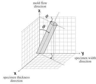
Figure 1 shows fiber orientation in spherical coordinates where ªand ºare angles with respect to moldflow (z-axis) and width direction (y-axis), respectively. When fiber cross section elliptical shapes are assigned ‘a’ and ‘b’ for their short and long axes, respectively fiber orientations, ª (deg) with respect to mold flow direction are obtained from eq. (1):7)
ª¼arccosða=bÞ ð1Þ
This is assuming circularfiber cross sections.
Measurement accuracy offiber cross-sections depends on computer screen size, resolution of computer program in positioning ellipses and resolution of SEM photomicro-graphs. For the conditions of this experiment, ellipses could be sized in 650 nm increments, therefore error was within +/¹650 nm. Hence, the error in measuring ellipse short axis,
a (fiber diameter) was within +/¹5.7% since average fiber diameter (aavg) was measured to be 11.36 µm. Likewise, the average long axis of the ellipses, bavg was 23.19 µm, thus percent error for long axes was within+/¹2.8%.
Fiber angle orientation mapping shows the 3-phase GFRP-BMC has been found to exhibit a 3-layered flow pattern of [skin-core-skin] where the profile is inferred here as a solidification wavefront 3-D elliptical paraboloid resembling classical laminar flow through a conduit that can apparently be estimated by Navier-Stokes equations.
Picturing the mold cavity as a straight rectangular duct, there are factors to consider. First, the BMC is opaque and has low contrast between fiber and matrix. While the accepted transition Reynolds number (Re) from laminar to turbulent flow is³2300 for circular pipe,13)the thick paste 3-phase BMC injection-molded polymer composite exhibits extremely low Re ³2.4©10¹4 undergoing highly viscous laminar creep motion classified as Stokes Flow, and lower than 2-phase fiber-polymer systems without filler. Stokes Flow is typically accompanied by a thick boundary layer where viscous forces dominate over inertial forces.13)
These extremely lowRenumbers act as an advantage for homogeneity of the part since entrance length,Leat which the
flow pattern and boundary layer stabilize14) calculated for laminar flow13,15,16) is nearly negligible in comparison to mold cavity length. Therefore, to characterize the GFRP-BMCflow through a conduit, the velocity profile and itsflow parameters are estimated fromfiber angle distribution across gauge section thickness.
2. Experimental
2.1 Preparation of GFRP
Premix, Inc. of North Kingsville, Ohio, provided an injection molded BMC (bulk molding compound) consisting of: 13.95 mass% propylene glycol maleate polyester (33 mass%styrene solution), 13.95 mass% styrene butadiene copolymer (70 mass%styrene solution), 20.00 mass%Owens and Corning OCF-405 E-glass fibers, 47.10 mass% calcium carbonate filler (CaCO3), 0.35 mass% t-butyl perbenzoate, 0.10 mass% t-butyl peroctoate, 0.25 mass% carbon black pigment, 1.20 mass% calcium stearate, 3.00 mass% alumi-num silicate and 0.10 mass%magnesium oxide.1,2)
To obtain flow parameter approximations taking into account the non-Newtonian shear thinning behavior of the BMC paste, dynamic viscosity measurements of Couette flow were carried out by rheometer at Premix, Inc. A linear Arrhenius relationship between dynamic viscosity © (Pas) and shear rate £_ (s¹1) was obtained at 20°C where viscosity was 9.0©103<©<4.3©105Pas for shear rates between 102>£_>100s¹1. In the specimen, the £_ cannot be measured directly, but can be calculated from the measured average flow (bulk) velocity, Ub by the Mooney-Rabinowitsch equation:17)
_
£¼4Q=³R3¼8U
b=DH ð2Þ
where£_is referred to as“average shear rate”,Qis volumetric flow rate (m3/s),R is radius if circular pipe (m),Ubis bulk velocity (0.135 ms¹1), DH is hydraulic diameter (m), for a square duct equal to 4A/P where A is specimen cross sectional area and P is wetted perimeter calculated as total perimeter, 2(w+th),14) hence£_ is 206 s¹1. Interpolation of the Arrhenius relationship yields bulk viscosity ©b of 5.0© 103Pas which we will use for calculations. The polyester melt viscosity,©melt is³2 Pas at 163°C.
Volume fractions,Vfof the E-glassfibers, CaCO3filler and polymers with remaining components were 0.1317, 0.2902 and 0.5781, respectively.
Paste with 3.2 mmfibers was mixed in a double-arm sigma blade mixer for a total of 50 min at room temperature. The paste was allowed to stand for several hours and then injected molded into an ASTM D-638 family mold for dogbone-shaped specimens with a 3.03©105N (75 ton) New Britain with the following processing parameters: mold temperature 436 K (163°C), barrel temperature RT, injection pressure 3.506.90 MPa, shot time, ts=³2.0 s, hold time 15 s and cure time 1.52.0 min. Averagefiber length,lof about 1,000 fibers was measured to be 0.44 mm with a standard deviation of 0.203 mm by SEM.1,2)In general, two standard deviations comprise approximately 95% of the population, which is 0.04 mm<l<0.85 mm.
θ
φ
z
y
x specimen thickness
direction
specimen width direction mold flow
direction
Sample dimensions total length, gauge length, width and thickness were ³210, 100, 12.6, 3.3 mm, respectively, with cross-sectional area of 42.0 mm2 in the gauge length.
2.2 Scanning electron microscopy (SEM)
A Jeol JSM-35CF scanning electron microscope (SEM) was used to observe polished surfaces of the composite. Specimens were polished with alumina polishing paper with successive finesses and sputtered with Pt. A mosaic of SEM photos across the specimen thickness was assembled.
3. Results
3.1 Composite specimen thickness
Figure 2 shows position of mapping of SEM photomicro-graphs across the 3.3 mm thickness for GFRP-BMC
speci-men perpendicular to mold flow direction z-axis. This was sectioned into 24 areas from 1 to 24 to obtain effect of position across thickness.
Figure 3 shows the mapping, which to our knowledge is thefirst time GFRP-BMC compositesfiber orientation map is illustrated in the literature. Since the BMC is opaque and has low contrast between fiber and matrix, Fig. 3 is a mosaic of SEM photomicrographs put together where ª are measured by meticulously sizing and positioning ellipses over thefiber cross sections using powerpoint computer program. Mold flow direction is normal to the plane of the page. Across the 3.3 mm thickness fibers appear to have a fountain confi g-uration, the centerfibers appearing to have been pushed out perpendicular with respect to the flow at highest velocity decreasing near or to zero near the mold walls. Fiber density distribution is inhomogeneous. There are fiber-rich areas in most sections while notably sections 46 have low fiber density. Some fibers appear to have been bent in sections 68 or broken during the mixing and the injection molding process.
Figure 4 shows average measured angle, º (deg) with respect toy-axis, parallel to specimen width for each section through thickness, th. Standard deviations (deg, in brackets) show variations in º are wide due to the fountain flow nature of the BMC paste. Interestingly, the averageºdo not deviate much from the width direction, showing the shorter dimension (th=3.3 mm) controls, or squeezes the flow patterns. Note these standard deviations in angle º do not designate the preciseness of the ellipse measurement, they merely show variation in flow. Ellipse measurements are quite accurate to +/¹650 nm and are described in the introduction yielding+/¹5.7 and+/¹2.8%for ellipse short and long axes (a andb), respectively.
3.3 mm
12.6 mm mold flo
w direction
θ=0 de
g
GFRP-BMC
SEM mapping area
0.74 mm
z
x
y
section 1 section 24
Fig. 2 Position of SEM mapping site on cross-section normal to the mold flow direction of GFRP-BMC sample in gauge length.
Fig. 3 Mapping of cross-section of GFRP-BMC across thickness. Molding direction is normal to the plane of the page.
Fig. 4 Measured average angle,º(deg) with respect to specimen width direction (y-axis), for each section through thickness,th. Standard deviations are in brackets.
Figure 5 shows an SEM micrograph at higher magnifi ca-tion near the mold wall where manyfibers are highly oriented to the moldflow direction. The three markedfibers (lines) to the left have ratio of ellipse long and short axesb/a=1.18, 1.26 and 1.21, henceª=32.0, 37.2 and 34.6 deg, from mold flow direction respectively, while angle with respect toy-axis width direction, º=4, ¹5 and ¹10 deg. The three marked fibers to the right have b/a=1.016, 1.030 and 1.052, thus ª=10.4, 13.9 and 18.1 deg, while theirº=¹1, 2 and 0 deg, respectively. Figure 6 shows an area near the center of the specimen thickness where fibers are oriented more perpen-dicular to the mold flow direction with marked fibers from left to right havingb/a=5.24, 10.81 and 5.80, respectively, henceª=79.0, 84.7 and 80.1 deg, withº=¹13,¹17 and
¹18 deg.
4. Discussion
4.1 Calculation of bulk velocity through specimen Figure 7 shows flow through the ASTM D-638 dogbone specimen. Flow is from sections A¼B¼C. For simplicity, velocities were calculated ignoring the taper and possible backflow in‘C’section. Hence, time tofill the 100 mm gauge length cavity B-section,tBis calculated as:
tB¼tsðVB=VtotÞ ð3Þ
where tB,ts,VBand Vtotare: time tofill B-section (0.741 s), total shot time (2.0 s), B-section volume (4165 mm3) and total specimen volume (11,245 mm3), respectively. This yields B-section bulk velocity,UB=Ub(m s¹1):
Ub ¼LB=tB ð4Þ
where LB is 100 mm gauge length, therefore Ub= 0.135 ms¹1. Velocities of wider sections A and C were 0.0874 ms¹1.
To characterize theflow pattern in relation to otherfluids, pipe sizes and geometries the dimensionless Reynolds number is useful:
Re¼μUbDH=©b ð5Þ
When μ is density of paste (kg m¹3) assumed to be equal to that of the solid finished part (1725 kg/m3), Ub is bulk velocity (ms¹1), DH is hydraulic diameter and ©b is bulk viscosity (5.0©103Pas) of the non-Newtonian paste, the estimated Reynolds number is 2.44©10¹4 in the gauge length and 1.73©10¹4 in wider sections “A” and “C” characteristic of viscous laminar creep flow.13)
4.2 Velocity profile, primary (¤0:99Uc) and secondary (¤f) boundary layers
The assumption made here isfiber orientation at a location through the thickness correlates with velocity at that location setting no-slip boundary velocity of zero at mold walls. Total bulk velocity, Ub is set at the 0.135 ms¹1 since time to fill the mold is³2 s. Thefiber orientation at a point is actually dependent on the history of velocity gradients the fibers experience up to the point measured, however, those near the core center tend to be more perpendicular to the molding direction indicating an approximately parabolic wavefront pushing the fibers more perpendicular to the wavefront. To get velocity profile from ª, for each section 1 to 24 in Fig. 3, Hermans fiber orientation parameter, ©o=[cos2(ª)] is employed whereª are obtained from eq. (1) as in Figs. 5 and 6. The average orientation parameter for each section from 124 (Fig. 3), can be calculated in eq. (6):7)
y
x
φ
WD 15mm 20.0 kV 3000x 10
μ
m
Fig. 5 SEM micrograph showing highly orientedfiber cross-sections near the mold wall. Moldflowz-direction is normal to the plane of the page.
bulk velocity, Ub (ms-1) 0.135 0.087 0.087
A B C
100 mm gauge length 55 mm
55 mm
3.3 mm
19.1 mm x
y z
12.6 mm
flow
Le= 1.05 mm
Fig. 7 Schematic of laminar creep flow of GFRP-BMC paste through specimen during injection molding illustrating 3-D elliptical paraboloid wavefront in gauge length.
y
x
φ
WD 15mm 20.0 kV 500x 50
μ
m
©o;j¼ij½NðªijÞcos2ðªijÞ=ij½NðªijÞ ð6Þ
where N(ªij) is number of fibers in each section, and i and j are fiber, and section number, respectively. Hence, velocity for each section, vj is estimated from Ub. To fit data to inverted parabola, orientation parameter is inverted (1¹©o,j)avgin eq. (7):
vj¼ ½Ub=ðj½Nð©o;jÞð1©o;jÞ=24Þð1©o;jÞ ð7Þ
where (1¹©o)avg=(j[N(©o,j)(1¹©o,j)]/24). Figure 8
shows the velocity profile obtained normalized for Ub= 0.135 ms¹1; showing centerline mean (Uc=0.180 ms¹1) and maximum velocities, (Umax=0.202 ms¹1), respectively.
Assigning primary boundary layer as that of flow, past research indicates it would be quite thick since asRenumber decreases boundary layer thickness increases due to the large viscous displacement effect.18)
To estimate ¤ for the GFRP-BMC flowing through the rectangular duct therefore, we follow the tradition of taking the points on the experimental curve of Fig. 9 that are 99% of the centerline velocity, 0.99Uc.14)Graphical interpolation for designated left and right sides yields ¤0:99Uc;ðLÞ and ¤0:99Uc;ðRÞ=0.49 and 1.61 mm (¤0:99Uc;ðavgÞ=1.05 mm),
re-spectively (Fig. 9) encompassing ³67% of the thickness. This is characteristic of the laminar creepflow of the highly viscous BMC.
In addition, we define a secondary boundary layer, ¤f for fiber reinforced composites as the distance from the mold walls in which fibers remain highly oriented with the flow, agreeing with other composite systems.10,11) This is done simply from the “skins” in Fig. 9 as: ¤f,(L) and ¤f,(R)=0.14 and 0.27 mm, respectively, hence ¤f,(avg)= 0.20 mm. Here fibers are ª=0 to 20 deg with respect to the mold flow direction. This is apparent in the mosaic of Fig. 3.
4.3 Parabolic velocity profilefit of BMC pasteflow from experimental values
To solve for the Navier-Stokes equations, the experimental data isfit to a parabolic velocity profile in which the sum of velocities, vi must equal that from the experimental data. Figure 9 shows the plot of eq. (8):
vz¼Uc,calc½1 ð2x=thÞ2 ð8Þ
where iteration yields calculated centerline velocity (Uc,calc) of 0.194 ms¹1. Although the positions of the experimental maximum velocities are higher and lower than the calculated parabolicfit on left and right sides respectively of Fig. 9, the parabola appears to be a decent approximation of the 3-layer flow. The difference between the experimental and calculated velocity profiles can be explained by Fig. 10 where higher velocities above that of the parabolicfit are accompanied by lower fiber densities, μf(A) below the average (μf(A),avg) of 498 mm¹2(solid line) in sections 3 to 10. The lowμfappears
Ub= 0.135 ms-1
Uc= 0.180 ms-1
V
elocity
,
vz
/ ms
-1
δL,f
= 0.137 mm
δR,f
= 0.275 mm
δR,(0.99
U
c)
= 1.69 mm
0
0.1
0.2
δL,(0.99
U
c)
= 0.49 mm
Umax= 0.202 ms-1
-1.7
0
1.7
Position from centerline of thickness, x / mm
Fig. 8 Calculated velocity profile of GFRP-BMCflowing through gauge section of mold showing primary (¤0:99Uc), and secondary (¤f) boundary
layers for left (L) and right (R) specimen walls, respectively.
calculated experimental
Uc,calc= 0.194 ms-1
δ0.99
U
c,calc
= 1.50 mm
vz=Uc,calc[ 1 – (2x/th)2]
Ub=
0.135 ms-1
-1.7
0
0
1.7
0.1
0.2
V
elocity
,
vz
/ ms
-1
Position from centerline of thickness, x / mm
Fig. 9 Parabolic profilefit across the 3.3 mm specimen thickness.
Section through thickness ρf(A),calc=ρf(V)0.667= 156 mm-2
ρf(A),avg= 498 mm-2
0 10 20
0 200 400 600 800
Fiber density per
pendicular to mold
dir
ection,
ρf(A)
/ mm
-2
1000
Fig. 10 Measuredfiber density,μf(A) perpendicular to molding direction
across specimen thickness. Average, μf(A),avg (solid line); and that
calculated from the E-glassfiber volume fraction (Vf),μf(A),calc(dotted
line) are indicated.
to allow the paste toflow faster through the mold causing the sparsefibers to be pushed out at higher angles perpendicular to the flow as shown in the Fig. 3 exhibiting a fountain configuration. On the other hand, on the right side of Fig. 9 lower velocities are accompanied by higher μf(A) above μf(A),avgin sections 12 to 23 causing higher resistance toflow and lower velocities than the parabolic fit.
For the parabolicfit, boundary conditionsvz=0, are set at mold walls x= +/¹th. Figure 9 shows calculated primary boundary layers ¤0:99Uc;calc are 1.50 mm (3.00 mm total)
extending throughout most of the thickness.
4.4 Approximating effective viscosity,©effat mold walls by steady-state Navier-Stokes equation
Picturing the BMC paste as forming a thin melt layer with lower viscosity within ¤fat the mold walls assisting to push the ultra-high viscosity core into the mold; it seems logical effective viscosity, ©eff at the mold walls can be estimated from injection pressure,¤Pusing the Navier-Stokes equation. Forflow along thez-axis:19)
μgz¤P=¤zþ©ð¤2vz=¤x2þ¤2vz=¤y2þ¤2vz=¤z2Þ
¼μðdvz=dtÞ ð9Þ
where the terms are: gravitational, pressure, viscous and acceleration forces per unit volume. Although the paste is a non-Newtonian shear thinningfluid20) and there are temper-ature gradients, this is beyond the scope of this study and seems to be taken into account in the frozenfiber orientation. Since the density of the thick BMC paste is approximately equal to that of the molded product because it contains 67.1 mass% hard components of glass fiber (20 mass%) and CaCO3filler (47.1 mass%) and only³28 mass%polymer, the Navier-Stokes equations are simplified as an incompressible Newtonianfluid with negligible gravitational effects eq. (9):
¤P=¤z¼©ð¤2v
z=¤x2þ¤2vz=¤y2Þ ð10Þ
where the velocity profile for laminarflow is approximated as the 3-D elliptical paraboloid:
vz¼Uc,calc½1 ð2x=thÞ2 ð2y=wÞ2 ð11Þ
whereUc,calcis 0.194 ms¹1. Substituting eq. (11) into eq. (10) 2nd order implicit differentiation yields:
¤P=¤z¼8©Uc,calc½ð1=thÞ2þ ð1=wÞ2 ð12Þ
The pressure drop across the three sections,‘A’,‘B’and‘C’ therefore is the sum:
ð¤P=¤zÞtot¼kð¤P=¤zÞk ðk goes from A to CÞ ð13Þ
Rearranging, we obtain effective viscosity, ©eff as a function of injection pressure,¤P:
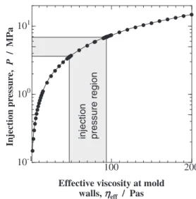
©eff¼ ð¤P=¤zÞtot=8f2Uc,A½ð1=thAÞ2þ ð1=wAÞ2
þUc,B½ð1=thBÞ2þ ð1=wBÞ2g ð14Þ where Uc,A=Uc,C=0.126 ms¹1, Uc,B=0.194 ms¹1 and ¤z=total specimen length,L (0.220 m). The plot in Fig. 11 shows the relation yielding effective viscosity range at mold walls estimated as 47.6<©eff<93.9 Pas (©eff,(avg)= 70.8 Pas) that must be overcome by the 3.5<¤P<6.9 MPa injection pressures. Exceeding the polyester melt viscosity of
³2 Pas, this seems a decent approximation since additives of
shrinkage control, cross-linking, thickening and mold release agents, with pigment and filler all play a role in increasing viscosity above the polymer melt.
4.5 Hydraulic head pressure loss and entrance length Since the present definitions of entrance length, Le and hydraulic head pressure loss,Plossare functions of the friction factor,f21) which depends primarily on theflow conditions at the duct walls, ©eff=70.8 Pas is used. Ploss of the paste entering section “A” at the gate can be calculated by the Darcy-Weisbach equation valid for duct flows of any cross section for laminar and turbulentflow:18)
Ploss¼fðL=DHÞðμUb2=2Þ ð15Þ
where μ is density of the paste. Friction coefficient for laminar flow calculated by f=64/Re15,16,22) is 5420 hence,
Ploss is 1.32 MPa. Thus,Plossis calculated to be 1938% of the 3.506.90 MPa injection mold pressure.
In addition, entrance length at which the boundary layer stabilizes,Lefor laminarflow is:13,15,16)
Le=DH¼0:06Re ð16Þ
Using this equation with ©eff=70.8 Pas,Leis calculated to be only 0.0054 mm for entering either sections “A” or “B” (Fig. 7), (0.0020.005% of length) indicating primary boundary layer, ¤0:99Uc and flow is approximately constant
and stable throughout the entire 210 mm length. This calculation indicates a steady-state flow condition of the fibers probably contributing to the excellent flow character-istics of BMCs that make them well-suited for injection-molded parts requiring precise dimensions and detail.
5. Conclusions
In conclusion, velocity profile of highly-filled GFRP-BMC that exhibits the laminar creepflow through rectangular duct-shaped specimen during injection molding from SEM fiber orientation mapping has been investigated. To our knowledge there is no or little research on estimating velocity profile fromfiber orientation mapping of GFRP-BMCs.
Injection pr
essur
e,
P
/ MP
a
Effective viscosity at mold walls,ηηeff / Pas
100 200
10-1 100 101
injection pressure region
(1) The BMC was found to exhibit a 3-layered [skin-core-skin]flow pattern that resembles classical laminarflow through a conduit and there was decent agreement with a parabolic curvefit. Variations from a perfect parabola were attributed to fiber density gradients across the specimen thickness. The subsequent Navier-Stokes calculation appeared to reliably estimate viscosity of melt layer at the mold walls.
(2) Mapping apparently allowed primary and secondary boundary layer values for flow and fiber orientation, respectively to be obtained. Primary boundary layer for fiber flow was estimated to stabilize at only 0.002 0.005% of the specimen length from entrance length calculations explaining the excellent flow character-istics of BMCs. Secondary boundary layer for fiber orientation was found to agree with that of unfilled GFRPs at 48% of the thickness. Thefiber orientation mapping appeared to provide specific information about fiber distributions and a decent approximation of flow parameters.
Acknowledgements
The authors extend their sincere gratitude to Shota Iizuka, M.S. and Ms. Miharu Seto for their great assistance with the electron microscope. The authors gratefully thank the staff of Premix, Inc. for preparation and viscosity measurements of the materials. The authors sincerely thank Dr. Keisuke Iwata of Tokai University and Professors Anne Hiltner and Eric Baer of Case Western Reserve University for their help.
REFERENCES
1) M. Faudree and Y. Nishi:Mater. Trans.51(2010) 23042310. 2) M. Faudree and Y. Nishi:Mater. Trans.53(2012) 14121419. 3) J. P. Greene and J. O. Wilkes:Polym. Eng. Sci.37(1997) 590602. 4) S. Toll and P. O. Andersson:Polym. Compos.14(1993) 116125. 5) S. Toll and P. O. Andersson:Composites22(1991) 298306. 6) J. L. Thomason:Compos. Sci. Technol.59(1999) 23152328. 7) J. L. Thomason:Composites A39(2008) 17321738. 8) H. L. Cox:Brit. J. Appl. Phys.3(1952) 7279.
9) H. Krenchel:Fibre Reinforcement, (Copenhagen: Akademisk Forlag, 1964).
10) M. Akay and D. Barkley:J. Mater. Sci.26(1991) 27312742. 11) B. E. VerWeyst, C. L. Tucker, III, P. H. Foss and J. F. O’Gara: Intl.
Polym. Process.4(1999) 409420.
12) C. A. Hieber and S. F. Shen:J. Non-Newtonian Fluid Mech.7(1980) 132.
13) F. M. White: Fluid Mechanics, 4th Edition, (New York: WCB/ McGraw-Hill, 1999) p. 326331.
14) F. Anselmet, F. Ternat, M. Amielh, O. Boiron, P. Boyer and L. Pietri: C. R. Mecanique337(2009) 573584.
15) H. Schlichting: Boundary Layer Theory, 7th Edition, (New York: McGraw-Hill, 1979).
16) F. M. White:Viscous Fluid Flow, 2nd Edition, (New York: McGraw-Hill, 1991).
17) E. T. Severs and J. M. Austin:Ind. Eng. Chem.46(1954) 23692375. 18) F. M. White: Fluid Mechanics, 4th Edition, (New York: WCB/
McGraw-Hill, 1999) p. 428.
19) F. M. White: Fluid Mechanics, 4th Edition, (New York: WCB/ McGraw-Hill, 1999) p. 228.
20) N. S. Martys, W. L. George, B. W. Chun and D. Lootens:Rheol. Acta 49(2010) 10591069.
21) J. P. Du Plessis and M. R. Collins: N and O Rheo.9(1992) 1116. 22) F. M. White: Fluid Mechanics, 4th Edition, (New York: WCB/
McGraw-Hill, 1999) p. 342.