Optimization for Statistical Machine Translation: A Survey

Translation: A Survey

Graham Neubig

Graduate School of Information Science Nara Institute of Science and Technology

Taro Watanabe

In statistical machine translation (SMT), the optimization of the system parameters to maximize translation accuracy is now a fundamental part of virtually all modern systems. In this article, we survey 12 years of research on optimization for SMT, from the seminal work on discriminative models (Och and Ney 2002) and minimum error rate training (Och 2003), to the most recent advances. Starting with a brief introduction to the fundamentals of SMT systems, we follow by covering a wide variety of optimization algorithms for use in both batch and online optimization. Specifically, we discuss losses based on direct error minimization, maximum likelihood, max-imum margin, risk minimization, ranking, and more, along with the appropriate methods for minimizing these losses. We also cover recent topics, including large-scale optimization, non-linear models, domain-dependent optimization, and the effect of MT evaluation measures or search on optimization. Finally, we discuss the current state of affairs in MT optimization, and point out some unresolved problems that will likely be the target of further research in optimization for MT.

1. Introduction

Machine translation (MT) has long been both one of the most promising applications of natural language processing technology and one of the most elusive. However, over approximately the past decade, huge gains in translation accuracy have been achieved (Graham et al. 2014), and commercial systems deployed for hundreds of language pairs are being used by hundreds of millions of users. There are many reasons for these advances in the accuracy and coverage of MT, but among them two particularly stand out: statistical machine translation (SMT) techniques that make it possible to learn statistical models from data, and massive increases in the amount of data available to learn SMT models.

∗8916-5 Takayama-cho, Ikoma, Nara, Japan. E-mail:[email protected].

∗∗6-10-1 Roppongi, Minato-ku, Tokyo, Japan. E-mail:[email protected].

This work was mostly done while the second author was affiliated with the National Institute of Information and Communications Technology, 3-5 Hikaridai, Seika-cho, Soraku-gun, Kyoto, 619-0289, Japan.

Submission received: 3 June 2014; revised version received: 18 March 2015; accepted for publication: 11 October 2015.

Within the SMT framework, there have been two revolutions in the way we math-ematically model the translation process. The first was the pioneering work of Brown et al. (1993), who proposed the idea of SMT, and described methods for estimation of the parameters used in translation. In that work, the parameters of a word-based generative translation model were optimized to maximize the conditional likelihood of the training corpus. The second major advance in SMT is the discriminative training framework proposed by Och and Ney (2002) and Och (2003), who propose log-linear models for MT, optimized to maximize either the probability of getting the correct sentence from a k-best list of candidates, or to directly achieve the highest accuracy over the entire corpus. By describing the scoring function for MT as a flexibly parameterizable log-linear model, and describing discriminative algorithms to optimize these parameters, it became possible to think of MT like many otherstructured predictionproblems, such as POS tagging or parsing (Collins 2002).

However, within the general framework of structured prediction, MT stands apart in many ways, and as a result requires a number of unique design decisions not neces-sary in other frameworks (as summarized in Table 1). The first is thesearch spacethat must be considered. The search space in MT is generally too large to expand exhaus-tively, so it is necessary to decide which subset of all the possible hypotheses should be used in optimization. In addition, the evaluation of MT accuracy is not straight-forward, with automatic evaluation measures for MT still being researched to this day. From the optimization perspective, even once we have chosen an automatic evaluation metric, it is not necessarily the case that it can be decomposed for straightforward integration with structured learning algorithms. Given this evaluation measure, it is necessary to incorporate it into aloss functionto target. The loss function should be closely related to the final evaluation objective, while allowing for the use of efficient optimization algorithms. Finally, it is necessary to choose anoptimization algorithm. In many cases it is possible to choose a standard algorithm from other fields, but there are also algorithms that have been tailored towards the unique challenges posed by MT.

Table 1

A road map of the various elements that affect MT optimization.

Which Loss Functions? Which Optimization Algorithm? Error (§3.1) Minimum Error Rate Training (§5.1) Softmax (§3.2) Gradient-based Methods (§5.2, §6.5) Risk (§3.3) Margin-based Methods (§5.3) Margin, Perceptron (§3.4) Linear Regression (§5.4) Ranking (§3.5) Perceptron (§6.2) Minimum Squared Error (§3.6) MIRA (§6.3)

AROW (§6.4)

Which Evaluation Measure? Which Hypotheses to Target? Corpus-level, Sentence Level (§2.5) k-best vs. Lattice vs. Forest (§2.4) BLEU and Approximations (§2.5.1, §2.5.2) Mergedk-bests (§5)

Other Measures (§8.3) Forced Decoding (§2.4), Oracles (§4)

Other Topics:

Large Data Sets (§7), Non-linear Models (§8.1),

In this article, we survey the state of the art in machine translation optimization in a comprehensive and systematic fashion, covering a wide variety of topics, with a unified set of terminology. In Section 2, we first provide definitions of the problem of machine translation, describe briefly how models are built, how features are defined, and how translations are evaluated, and finally define the optimization setting. In Section 3, we next describe a variety of loss functions that have been targeted in machine translation optimization. In Section 4, we explain the selection of oracle translations, a non-trivial process that directly affects the optimization results. In Section 5, we describe batch optimization algorithms, starting with the popular minimum error rate training, and continuing with other approaches using likelihood, margin, rank loss, or risk as objectives. In Section 6, we describe online learning algorithms, first explaining the relationship between corpus-level optimization and sentence-level optimization, and then moving on to algorithms based on perceptron, margin, or likelihood-based objectives. In Section 7, we describe the recent advances in scaling training of MT systems up to large amounts of data through parallel computing, and in Section 8, we cover a number of other topics in MT optimization such as non-linear models, domain adaptation, and the relationship between MT evaluation and optimization. Finally, we conclude in Section 9, overviewing the methods described, making a brief note about which methods see the most use in actual systems, and outlining some of the unsolved problems in the optimization of MT systems.

2. Machine Translation Preliminaries and Definitions

Before delving into the details of actual optimization algorithms, we first introduce pre-liminaries and definitions regarding MT in general and the MT optimization problem in particular. We focus mainly on the aspects of MT that are relevant to optimization, and readers may refer to Koehn (2010) or Lopez (2008) for more details about MT in general. 2.1 Machine Translation

Machine translation is the problem of automatically translating from one natural lan-guage to another. Formally, we define this problem by specifyingFto be the collection of all source sentences to be translated,f ∈F as one of the sentences, andE(f) as the collection of all possible target language sentences that can be obtained by translatingf. Machine translation systems perform this translation process by dividing the translation of a full sentence into the translation and recombination of smaller parts, which are represented ashidden variables, which together form aderivation.

For example, in phrase-based translation (Koehn, Och, and Marcu 2003), the hidden variables will be the alignment between the phrases of the source and target sentences, and in tree-based translation models (Yamada and Knight 2001; Chiang 2007), the hidden variables will represent the latent tree structure used to generate the translation. We will defineD(f) to be the space of possible derivations that can be acquired from source sentencef, andd∈D(f) to be one of those derivations. Any particular deriva-tiond will correspond to exactly onee∈E(f), although the opposite is not true (the derivation uniquely determines the translation, but there can be multiple derivations corresponding to a particular translation). We also define tuple he,di consisting of a target sentence and its corresponding derivation, andT(f)⊆E(f)×D(f) as the set of all of these tuples.

translations. In order to do so, in machine translation it is common to define alinear model that determines the score of each translation candidate. In this linear model we first define anM-dimensionalfeature vectorfor each output and its derivation as h(f,e,d) :F×E×D→_RM_{. For each feature, we also define a corresponding weight,} resulting in an M-dimensional weight vector w∈RM. Based on these feature and

weight vectors, we proceed to define the problem of selecting the best he,di as the following maximization problem

heˆ, ˆdi= arg max he,di∈T(f)

w>h(f,e,d) (1)

where the dot product of the parameters and features is equivalent to the score assigned to a particular translation.

The optimization problem that we will be surveying in this article is generally concerned with finding the most effective weight vector w from the set of possible weight vectorsRM.1Optimization is also widely calledtuningin the SMT literature. In

addition, because of the exponentially large number of possible translations inE(f) that must be considered, it is necessary to take advantage of the problem structure, making MT optimization an instance ofstructured learning.

2.2 Model Construction

The first step of creating a machine translation system is model construction, in which translation models(TMs) are extracted from a large parallel corpus. The TM is usually created by first aligning the parallel text (Och and Ney 2003), using this text to extract multi-word phrase pairs or synchronous grammar rules (Koehn, Och, and Marcu 2003; Chiang 2007), and scoring these rules according to several features explained in more detail in Section 2.3. The construction of the TM is generally performed first in a manner that does not directly consider the optimization of translation accuracy, followed by an optimization step that explicitly considers the accuracy achieved by the system.2In this survey, we focus on the optimization step, and thus do not cover elements of model construction that do not directly optimize an objective function related to translation accuracy, but interested readers can reference Koehn (2010) for more details.

In the context of this article, however, the TM is particularly important in the role it plays in defining our derivation spaceD(f). For example, in the case of phrase-based translation, only phrase pairs included in the TM will be expanded during the process of searching for the best translation (explained in Section 2.4).

This has major implications from the point of view of optimization, the most impor-tant of which being that we must use separate data for training the TM and optimizing the parametersw. The reason for this lies in the fact that the TM is constructed in such a way that allows it to “memorize” long multi-word phrases included in the training data. Using the same data to train the model parameters will result inoverfitting, learning parameters that heavily favor using these memorized multi-word phrases, which will not be present in a separate test set.

1 It should be noted that although most work on MT optimization is concerned with linear models (and thus we will spend the majority of this article discussing optimization of these models), optimization using non-linear models is also possible, and is discussed in Section 8.1.

The traditional way to solve this problem is to train the TM on a large parallel corpus on the order of hundreds of thousands to tens of millions of sentences, then perform optimization of parameters on a separate set of data consisting of around one thousand sentences, often called thedevelopment set. When learning the weights for larger feature sets, however, a smaller development set is often not sufficient, and it is common to performcross-validation, holding out some larger portion of the training set for parameter optimization. It is also possible to performleaving-one-outtraining, where counts of rules extracted from a particular sentence are subtracted from the model before translating the sentence (Wuebker, Mauser, and Ney 2010).

2.3 Features for Machine Translation

Given this overall formulation of MT, the featuresh(f,e,d) that we choose to use to represent each translation hypothesis are of great importance. In particular, with regard to optimization, there are two important distinctions between types of features: local vs. non-local, and dense vs. sparse.

With regard to the first distinction,local features, such as phrase translation prob-abilities, do not require additional contexts from other partial derivations, and they are computed independently from one another. On the other hand, when features for a particular phrase pair or synchronous rule cannot be computed independently from other pairs, they are callednon-local features. This distinction is important, as local features will not result in an increase in the size of the search space, whereas non-local features have the potential to make search more difficult.

The second distinction is betweendense features, which define a small number of highly informative feature functions, andsparse features, which define a large number of less informative feature functions. Dense features are generally easier to optimize, both from a computational point of view because the smaller number of features re-duces computational and memory requirements, and because the smaller number of parameters reduces the risk of overfitting. On the other hand, sparse features allow for more flexibility, as their parameters can be directly optimized to increase translation accuracy, so if optimization is performed well they have the potential to greatly increase translation accuracy. The remainder of this section describes some of the widely used features in more detail.

2.3.1 Dense Features. Dense features, which are generally continuously valued and present in nearly all translation hypotheses, are used in the majority of machine trans-lation systems. The most fundamental set of dense features are phrase/ruletranslation probabilities or relative frequencies in which the log of sentence-wise probability distributionsp(f|e) andp(e|f), are split into the sum of phrase or rule log probabilities

hφ(f,e,d)=

X

hα,βi∈d

logpφ(α|β), hφ0(f,e,d)=P_h

α,βi∈dlogpφ0(β|α) (2)

Hereαandβare the source and target sides of a phrase pair or rule. These features are estimated using counts of each phrase derived from the training corpus as follows:

pφ(α|β)= count(

α,β) P

α0count(α0,β), pφ

0(β|α)= _Pcount(α,β)

In addition, it is also common to use lexical weighting, which estimates parameters for each phrase pair or rule by further decomposing them into word-wise probabilities (Koehn, Och, and Marcu 2003). This helps more accurately estimate the reliability of phrase pairs or rules that have low counts. It should be noted that all of these features can be calculated directly from the rules themselves, and are thus local features.

Another set of important features are language models (LMs), which capture the fluency of translatione, and are usually modeled byn-grams

hlm(f,e,d)=

|e|

X

i=1

logplm(ei|ei−i−n+1 1) (4)

Note that the n-gram LM is computed over eregardless of the boundaries of phrase pairs or rules in the derivation, and is thus a non-local feature.

Then-gram language model assigns higher penalties for longer translations, and it is common to add a word penalty feature that measures the length of translation e to compensate for this. Similarly, phrase penalty or rule penalty features express the trade-off between longer or shorter derivations. There exist other features that are dependent on the underlying MT system model. Phrase-based MT heavily relies on the distortion probabilitiesthat are computed by the distance on the source side of target-adjacent phrase pairs. More refinedlexicalized reordering modelsestimate the parameters from the training data based on the relative distance of two phrase pairs (Tillman 2004; Galley and Manning 2008).

2.3.2 Sparse features.Although dense features form the foundation of most SMT systems, in recent years the ability to define richer feature sets and directly optimize the system using rich features has been shown to allow for significant increases in accuracy. On the other hand, large and sparse feature sets make the MT optimization problem signifi-cantly harder, and many of the optimization methods we will cover in the rest of this survey are aimed at optimizing rich feature sets.

The first variety of sparse features that we can think of are phrase features or rule features, which count the occurrence of every phrase or rule. Of course, it is only possible to learn parameters for a translation rule if it exists in the training data used in optimization, so when using a smaller data set for optimization it is difficult to robustly learn these features. Chiang, Knight, and Wang (2009) have noted that this problem can be alleviated by only selecting and optimizing the more frequent of the sparse features. Simianer, Riezler, and Dyer (2012) also propose features using the “shape” of translation rules, transforming a rule

X→ hne X₁ pas, did not X₁i (5) into a string simply indicating whether each word is a terminal (T) or non-terminal (N)

N→ hT N T, T T Ni (6)

Count-based features can also be extended to cover other features of the translation, such as phrase or rule bigrams, indicating which phrases or rules tend to be used together (Simianer, Riezler, and Dyer 2012).

similar to lexical weighting, focus on the correspondence between the individual words that are included in a phrase or rule. The simplest variety of lexical features remembers which source wordsf are aligned with which target words e, and fires a feature for each pair. It is also possible to condition lexical features on the surrounding context in the source language (Chiang, Knight, and Wang 2009; Xiao et al. 2011), fire features between every pair of words in the source or target sentences (Watanabe et al. 2007), or integrate bigrams on the target side (Watanabe et al. 2007). Of these, the former two can be calculated from source and local target context, but target bigrams require target bigram context and are thus non-local features.

One final variety of features that has proven useful is syntax-based features (Blunsom and Osborne 2008; Marton and Resnik 2008). In particular, phrase-based and hierarchical phrase-based translations do not directly consider syntax (in the linguistic sense) in the construction of the models, so introducing this information in the form of features has a potential for benefit. One way to introduce this information is to parse the input sentence before translation, and use the information in the parse tree in the calculation of features. For example, we can count the number of times a phrase or translation rule matches, or partially matches (Marton and Resnik 2008), a span with a particular label, based on the assumption that rules that match a syntactic span are more likely to be syntactically reasonable.

2.3.3 Summary features.Although sparse features are useful, training of sparse features is an extremely difficult optimization problem, and at this point there is still no method that has been widely demonstrated as being able to robustly estimate the parameters of millions of features. Because of this, a third approach of first training the parameters of sparse features, then condensing the sparse features into dense features and performing one more optimization pass (potentially with a different algorithm), has been widely used in a large number of research papers and systems (Dyer et al. 2009; He and Deng 2012; Flanigan, Dyer, and Carbonell 2013; Setiawan and Zhou 2013). A dense feature created from a large group of sparse features and their weights is generally called a summary feature, and can be expressed as follows

hsum(f,e,d)=w>sparsehsparse(f,e,d) (7)

There has also been work that splits sparse features into not one, but multiple groups, creating a dense feature for each group (Xiang and Ittycheriah 2011; Liu et al. 2013).

2.4 Decoding

Given an input sentence f, the task of decoding is defined as an inference problem of finding the best scoring derivationheˆ, ˆdiaccording to Equation (1). In general, the inference is intractable if we enumerate all possible derivations in T(f) and rank each derivation by the model. We assume that a derivation is composed of a set of steps

d=d1,d2,· · ·,d|d| (8)

each feature function can be decomposed over each step, and Equation (1) can be expressed by

heˆ, ˆdi= arg max he,di∈T(f)

|w|

X

i wi

|d|

X

j=1

hi(dj,ρi(dj−1 1)) (9)

wherehi(dj,ρi(d j−1

1 )) is a feature function for thejth step decomposed from the global

feature function of hi(f,e,d). As mentioned in the previous section, non-local fea-tures require information that cannot be calculated directly from the rule itself, and

ρ_i(dj−₁ 1) is a variable that defines the residual information to score thisith feature func-tion using the partial derivafunc-tion dj−₁ 1 (Gesmundo and Henderson 2011; Green, Cer, and Manning 2014). For example, in phrase-based translation, for ann-gram language model feature,ρ_i(dj−₁ 1) will be then−1 word suffix of the partial translation (Koehn, Och, and Marcu 2003). The local feature functions, such as phrase translation probabili-ties in Section 2.3.1, require no context from partial derivations, and thusρ_i(dj−₁ 1)=∅.

The problem of decoding is treated as a search problem in which partial derivations ˙

d together withρ_i( ˙d) in Equation (9) are enumerated to form hypotheses or states. In phrase-based MT, search is carried out by enumerating partial derivations in left-to-right order on the target side while remembering the translated source word positions. Similarly, the search in MT with synchronous grammars is performed by using the CYK+ algorithm (Chappelier and Rajman 1998) on the source side and generating partial derivations for progressively longer source spans. Because of the enormous search space brought about by maintainingρ_i( ˙d) in each partial derivation,beam search is used to heuristically prune the search space. As a result, the search isinexactbecause of thesearch errorcaused by heuristic pruning, in which the best scoring hypothesis is not necessarily optimal in terms of given model parameters.

The search is efficiently carried out by merging equivalent states encoded as ρ

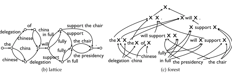
(Koehn, Och, and Marcu 2003; Huang and Chiang 2007), and the space is succinctly represented by compact data structures, such asgraphs(Ueffing, Och, and Ney 2002) (orlattices) in phrase-based MT (Koehn, Och, and Marcu 2003) andhypergraphs(Klein and Manning 2004) (or packed forests) in tree-based MT (Huang and Chiang 2007). These data structures may be directly used as compact representations of all derivations for optimization.

the delegation of china will support the chair in full . the chinese delegation will fully support the chair . the chinese delegation will fully support the presidency . the delegation of china will in full support the presidency . the china delegation will in full support the chair .

(a)k-best

the delegation

of china chinese

china

chinese _delegation will fully

in full

support

support

fully

in full the chair

the presidency . support the chair

(b) lattice

will support

the presidency the chair will

in full fully delegation china

the

chinese the

X X .

X ofX

X X X X X supportX

X

X willX . X supportX

(c) forest

Figure 1

Example of ak-best list, lattice, and forest.

Another class of decoding problem isforced decoding, in which the output from a decoder is forced to match with a reference translation of the input sentence. In phrase-based MT, this is implemented by adding additional features to reward hypotheses that match with the given target sentence (Liang, Zhang, and Zhao 2012; Yu et al. 2013). In MT using synchronous grammars, it is carried out bybiparsingover two languages, for instance, by a variant of the CYK algorithm (Wu 1997) or by a more efficient two-step algorithm (Dyer 2010b; Peitz et al. 2012). Even if we perform forced decoding, we are still not guaranteed that the decoder will be able to produce the reference translation (because of unknown words, reordering limits, or other factors). This problem can be resolved by preserving the prefix of partial derivations (Yu et al. 2013), or by allowing approximate matching of the target side (Liang, Zhang, and Zhao 2012). It is also possible to create aneighborhoodof a forced decoding derivation by adding additional hyperedges to the true derivation, which allows for efficient generation of negative examples for discriminative learning algorithms (Xiao et al. 2011).

2.5 Evaluation

Once we have a machine translation system that can produce translations, we next must performevaluationto judge how good the generated translations actually are. As the final consumer of machine translation output is usually a human, the most natural form of evaluation is manual evaluation by human annotators. However, because human evaluation is expensive and time-consuming, in recent years there has been a shift to automatic calculation of the quality of MT output.

In general, automatic evaluation measures use a set of data consisting of Ninput sentencesF=nf(i)oN

i=1, each of which having areference translationE=

e(i) N_i=1that was created by a human translator. The inputFis automatically translated using a ma-chine translation system to acquire MT results ˆE=

ˆ

many ways to translate a particular sentence, it is also possible to perform evaluation with multiple references created by different translators. There has also been some work on encoding a huge number of references in a lattice, created either by hand (Dreyer and Marcu 2012) or by automatic paraphrasing (Zhou, Lin, and Hovy 2006).

One major distinction between optimization measures is whether they are calcu-lated on thecorpus levelor thesentence level. Corpus-level measures are calculated by taking statistics over the whole corpus, whereas sentence-level measures are calculated by measuring sentence-level accuracy, and defining the corpus-level accuracy as the average of the sentence-level accuracies. All optimization algorithms that are applicable to corpus-level measures are applicable to sentence-level measures, but the opposite is not true, making this distinction important from the optimization point of view.

The most commonly used MT evaluation measure BLEU (Papineni et al. 2002) is defined on the corpus level, and we will cover it in detail as it plays an important role in some of the methods that follow. Of course, there have been many other evaluation measures proposed since BLEU, with TER (Snover et al. 2006) and METEOR (Banerjee and Lavie 2005) being among the most widely used. The great majority of metrics other than BLEU are defined on the sentence level, and thus are conducive to optimization algorithms that require sentence-level evaluation measures. We discuss the role of evaluation in MT optimization more completely in Section 8.3.

2.5.1 BLEU.BLEU is defined as the geometric mean ofn-gram precisions (usually forn

from 1 to 4), and a brevity penalty to prevent short sentences from receiving unfairly high evaluation scores. For a single reference sentence eand a corresponding system output ˆe, we can definecn(ˆe) as the number ofn-grams in ˆe, andmn(e, ˆe) as the number ofn-grams in ˆethat matche

cn(ˆe)=|{gn∈e}|ˆ

mn(e, ˆe)=|{gn∈e} ∩ {ˆ g0n∈e}|

Here,{gn∈ˆe}and{g0n∈e}are multisets that can contain identicaln-grams more than once, and ∩is an operator for multisets that allows for consideration of multiple in-stances of the samen-gram.3_{Note that the total count for a candidaten-gram isclipped}

to be no more than the count in the reference translation. If we have a corpus of reference setsR={e(1)_{,. . .,e}(N)_{}, where each sentence hasMreferencese}(i)_={e(i)

1 ,. . .,e (i)

M}, the BLEU score of the corresponding system outputs E={eˆ(1),. . ., ˆe(N)} can be defined as

BLEU(E, ˆE)=

4

Y

n=1

PN

i=1mn({e1(i),. . .,e (i)

M}, ˆe(i))

PN

i=1cn(ˆe(i))

!1₄

·BP(E, ˆE) (10)

where the first term corresponds to geometric mean of the n-gram precisions, and the second term BP(E, ˆE) is thebrevity penalty. The brevity penalty is necessary here because evaluation of precision favors systems that output only the words and phrases that have high accuracy, and avoids outputting more difficult-to-translate content that

3 We let #A(a) denote the number of timesaappeared in a multisetA, and define:|A|=

P

a#A(a),

might not match the reference. The brevity penalty prevents this by discounting outputs that are shorter than the reference

BP(E, ˆE)=min (

1, exp 1− PN

i=1|e˜(i)|

PN

i=1|eˆ(i)|

!)

(11)

where ˜e(i)is defined as the longest reference with a length shorter than or equal to ˆe(i).

2.5.2 BLEU+1.One thing to notice here is that BLEU is calculated by taking statistics over the entire corpus, and thus it is a corpus-level measure. There is nothing inherently preventing us from calculating BLEU on a single sentence, but in the single-sentence case it is common for the number of matches of higher ordern-grams to become zero, resulting in a BLEU score of zero for the entire sentence. One common solution to this problem is the use of a smoothed version of BLEU, commonly referred to as BLEU+1 (Lin and Och 2004). In BLEU+1, we add one to the numerators and denominators of eachn-gram of order greater than one

c0_n(ˆe)=|{gn∈e}|ˆ +δ(n>1)

m_n0(e, ˆe)=|{gn∈e} ∩ {ˆ g0n∈e}|+δ(n>1)

whereδ(·) is a function that takes a value of 1 when the corresponding statement is true. We can then re-define a sentence-level BLEU using these smoothed counts

BLEU’(e, ˆe)=

4

Y

n=1

m0_n({e1,. . .,eM}, ˆe) c0

n(ˆe)

1₄

·BP(e, ˆe) (12)

and the corpus-level evaluation can be re-defined as the average of sentence level evaluations

BLEU’(E, ˆE)= 1 N

N

X

i=1

BLEU’(e(i), ˆe(i)) (13)

It has also been noted, however, that the average of sentence-level BLEU+1 is not a very accurate approximation of corpus-level BLEU, but by adjusting the smoothing heuristics it is possible to achieve a more accurate approximation (Nakov, Guzman, and Vogel 2012).

2.6 The Optimization Setting

During the optimization process, we will assume that we have some data consisting of sourcesF=nf(i)oN

i=1 with corresponding referencesE=

e(i) N

i=1 as defined in the

previous section, and that we would like to use these to optimize the parameters of the model. As mentioned in Section 2.5, it is also possible to use more than one reference translation in evaluation, but in this survey we will assume for simplicity of exposition that only one reference is used.

in Section 2.4. To express whether this effect is a positive or negative one, we define a loss function`(F,E;w) :FN_×EN_×

RM →Rthat provides a numerical indicator of

how “bad” the translations generated when we use a particularw are. As the goal of optimization is to achieve better translations, we would like to choose parameters that reduce this loss. More formally, we can cast the problem as minimizing the expectation of`(·), orrisk minimization:

ˆ

w=arg min

w∈RM

EPr(F,E)[`(F,E;w)] (14)

Here,Pr(F,E) is the true joint distribution over all sets of input and output sentences that we are likely to be required to translate. However, in reality we will not know the true distribution over all sets of sentences a user may ask us to translate. Instead, we have a single set of data (henceforth,training data), and attempt to find thewthat minimizes the loss on this data:

ˆ

w=arg min

w∈RM

`(F,E;w) (15)

Because we are now optimizing on a single empirically derived set of training data, this framework is calledempirical risk minimization.

In machine learning problems, it is common to introduceregularizationto prevent the learning of parameters that over-fit the training data. This gives us the framework of regularized empirical risk minimization, which will encompass most of the methods described in this survey, and is formalized as

ˆ

w=arg min

w∈RM

`(F,E;w)+λΩ(w) (16)

whereλis a parameter adjusting the strength of regularization, andΩ(w) is a regular-ization term, common choices for which include theL2 regularizerΩ2(w)= 12kwk22=

1

2w>w or the L1 regularizerΩ1(w)=kwk1=PMm=1|wm| (Tibshirani 1996; Chen and Rosenfeld 1999). Intuitively, if λ is set to a small value, optimization will attempt to learn awthat effectively minimizes loss on the training data, but there is a risk of over-fitting reducing generalization capability. On the other hand, ifλis set to a larger value, optimization will be less aggressive in minimizing loss on the training data, reducing over-fitting, but also possibly failing to capture useful information that could be used to improve accuracy.

3. Defining a Loss Function

3.1 Error

The first, and most straightforward, loss that we can attempt to optimize iserror(Och 2003). We assume that by comparing the decoder’s translation result ˆEwith the refer-enceE, we are able to calculate a function error(E, ˆE) :EN×EN→R≥0that describes the

extent of error included in the translations. For example, if we use the BLEU described in Section 2.5 as an evaluation measure for our system, it is natural to use 1−BLEU as an error function, so that as our evaluation improves, the error decreases. Converting this to a loss function that is dependent on the model parameters, we obtain the following loss expressing the error over the 1-best results obtained by decoding in Equation (1):

`_error(F,E,C;w)=error 

E, (

arg max he,di∈c(i)

w>h(f(i),e,d) )N

i=1



 (17)

Error has the advantage of being simple, easy to explain, and directly related to translation performance, and these features make it perhaps the most commonly used loss in current machine translation systems. On the other hand, it also has a large disadvantage in that the loss function expressed in Equation (17) is not convex, and most MT evaluation measures used in the calculation of the error function error(·) are not continuously differentiable. This makes direct minimization of error a difficult optimization problem (particularly for larger feature sets), and thus a number of other, easier-to-optimize losses are used as well.

A special instance of error, which is worth mentioning because of its relation to the methods we will introduce in the following sections, iszero–one loss. Zero–one loss focuses on whether anoracle translationis chosen as the system output. Oracle trans-lations can be vaguely defined as “good” transtrans-lations, such as the reference translation e(i), or perhaps the best translation in thek-best list (described in detail in Section 4). If we define the set of oracle translations for sentenceiaso(i), zero–one loss is defined by plugging the following zero–one error function into Equation (17):

error(E, ˆE)= 1 N

N

X

i=1

1−δ(ˆe(i)∈o(i))

(18)

where ˆe(i)is the one-best translation candidate, andδ(ˆe(i)∈o(i)_{) is one if ˆe}(i)_{is a member}

ofo(i)_{and zero otherwise.}

3.2 Softmax Loss

In particular, if we assume that MT is modeled according to the log-linear model

pw(e,d|f,c)=

exp(w>h(f,e,d)) P

he0_,d0_i∈cexp(w>h(f,e0,d0)) (19)

we can define softmax loss`_softmax(·) as follows:

`_softmax(F,E,C;w)=−1

N N

Y

i=1

X

he,di∈o(i)

pw(e,d|f(i),c(i)) (20)

=−1

N N

Y

i=1

P

he,di∈o(i)exp(w>h(f(i),e,d))

P

he,di∈c(i)exp(w>h(f(i),e,d))

(21)

From Equation (21) we can see that only the oracle translations contribute to the numerator, and all candidates inc(i)_{contributes to the denominator. Thus, intuitively,}

the softmax objective prefers parameter settings that assign high scores to the oracle translations, and lower scores to any other members ofc(i)_{that are not oracles.}

It should be noted that this loss can be calculated from ak-best list by iterating over the entire list and calculating the numerators and denominators in Equation (19). It is also possible, but more involved, to calculate over lattices or forests by using dynamic programming algorithms such as the forward–backward or inside–outside algorithms (Blunsom, Cohn, and Osborne 2008; Gimpel and Smith 2009).

3.3 Risk-Based Loss

In contrast to softmax loss, which can be viewed as a probabilistic version of zero–one loss,riskdefines a probabilistic version of the translation error (Smith and Eisner 2006; Zens, Hasan, and Ney 2007; Li and Eisner 2009; He and Deng 2012). Specifically, risk is based on the expected error incurred by a probabilistic model parameterized byw. This combines the advantages of the probabilistic model in softmax loss with the direct consideration of translation accuracy afforded by using error directly. In comparison to error, it also has the advantage of being differentiable, allowing for easier optimization. To define this error, we define a scaling parameterγ≥0 and use it in the calculation of each hypothesis’s probability

pγ,w(e,d|f,c)=

exp(γw>h(f,e,d)) P

he0_,d0_i∈

cexp(γw>h(f,e0,d

0₎₎ (22)

Given this probability, we then calculate the expected loss as follows:

`risk(F,E,C;γ,w)= _N1

N

X

i=1

E_pγ,w(e,d|f(i)_,c(i)₎[err(e(i),e)] (23)

= 1 N

N

X

i=1

X

he,di∈c(i)

In Equation (22), whenγ=0 regardless of parameters wevery hypothesis he,diwill be assigned a uniform probability, and whenγ=1 the probabilities are equivalent to those in the log-linear model of Equation (19). When γ→ ∞, the probability of the highest-scored hypothesis will approach 1, and thus our objective will approach the error defined in Equation (17). Thisγ can be adjusted in a way that allows for more effective search of the parameter space, as described in more detail in Section 5.5.

3.4 Margin-Based Loss

The zero–one loss in Section 3.1 was based on whether the oracle received a higher score than other hypotheses. The idea ofmargin, which is behind the classification paradigm ofsupport vector machines(SVMs) (Joachims 1998), takes this a step further, finding parameters that explicitly maximize the distance, or margin, between correct and incorrect candidates. The main advantage of margin-based methods is that they are able to consider the error function, and often achieve high accuracy. These advantages make margin-based methods perhaps the second most popular loss used in current MT systems after direct minimization of error.

This margin-based objective can be defined as the loss:

`_margin(F,E,C;w)= 1 N(C)

N

X

i=1

X

he∗_,d∗_i∈o(i)

X

he,di∈c(i)_\o(i)

maxn0,∆err(e(i),e∗,e)−w>∆h(f(i),e∗,d∗,e,d)o (25)

where we define

∆err(e,e∗,e0)=err(e,e0)−err(e,e∗) (26) ∆h(f,e∗,d∗,e0,d0)=h(f,e∗,d∗)−h(f,e0,d0) (27)

In Equation (25), we first specify that for each pair of oracle candidateso(i)_{, and}

non-oracle candidates c(i)_\o(i)_{, the margin w}>_{∆h(·) between oracle e}∗ _{and non-oracle e} should be greater than the difference in the error∆err(·).4_{We then define the loss as the}

total amount that this margin is violated. In this loss calculation, the number of pairs is

N(C)=PN

i=1|c(i)\o(i)| · |o(i)|. Note that here err(·) is not calculated on the corpus level,

but on the sentence level, and may not directly correspond to our corpus-level error error(·).

It is also common to consider the case where we calculate this loss with regards to only a single translation candidate and oracle, and this is often calledhinge loss. If we defineheˆ(i), ˆd(i)i ∈c(i)\o(i)as the 1-best translation candidate

heˆ(i), ˆd(i)i= arg max he,di∈c(i)_\o(i)

w>h(f(i),e,d) (28)

andhe∗(i)_,d∗(i)_{i ∈o}(i)_{as the oracle translation}

he∗(i),d∗(i)i=arg min he,di∈o(i)

err(e(i),e) (29)

the hinge loss can be defined as follows

`_hinge(F,E,C;w)= 1 N

N

X

i=1

maxn0,∆err(e∗(i),e∗,e)−w>∆h(f(i),e∗(i),d∗(i), ˆe(i), ˆd(i))o (30)

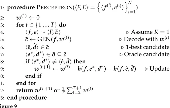
A special instance of this hinge loss that is widely used in machine translation, and machine learning in general, isperceptron loss (Liang et al. 2006), which further re-moves the term considering the error, and simply incurs a penalty if the 1-best candidate receives a higher score than the oracle

`_perceptron(F,E,C;w)= 1 N

N

X

i=1

maxn0,−w>∆h(f(i),e∗(i),d∗(i), ˆe(i), ˆd(i))o (31)

In addition to maximizing the margin itself, there has also been work on maximiz-ing the relative margin(Eidelman, Marton, and Resnik 2013). To explain the relative margin, we first define theworst hypothesisas

he˘(i), ˘d(i)i=arg max he,di∈c(i)

err(e(i),e) (32)

and then calculate the spread∆err(e(i)_{, ˙e}(i)_{, ˘e}(i)_{), which is the difference of errors}

be-tween the oracle hypothesis he˙(i)_{, ˙d}(i)_{i and worst hypothesis he˘}(i)_{, ˘d}(i)_{i. An additional}

term can then be added to the objective function to penalize parameter settings with large spreads. The intuition behind the relative margin criterion is that in addition to increasing the margin, considering the spread reduces the variance between the non-oracle hypotheses. Given an identical margin, having a smaller variance indi-cates that an unseen hypothesis will be less likely to pass over the margin and be misclassified.

3.5 Ranking Loss

particular pair of candidates in the training datahek,dkiandhek0,d_k0iis ranked in the

correct order, the following condition is satisfied:

err(e(i),ek)<err(e(i),ek0)

⇐⇒ w>h(f(i),ek,dk)>w>h(f(i),ek0,d_k0)

This can be expressed as

err(e(i),ek)<err(e(i),ek0)

⇐⇒ w>h(f(i),ek,dk)>w>h(f(i),ek0,d_k0)

⇐⇒ w>h(f(i),ek,dk)−w>h(f(i),ek0,d_k0)>0

⇐⇒ w>h(f(i),ek,dk)−h(f(i),ek0,d_k0)

>0 ⇐⇒ w>∆h(f(i),ek,dk,ek0,d_k0)>0

where∆h(f(i),ek,dk,ek0,d_k0) can be treated as training data to be classified using any

variety ofbinary classifier. Each binary decision made by this classifier becomes an individual choice, and thus the ranking loss is the sum of these individual losses. As the binary classifier, it is possible to use perceptron, hinge, or softmax losses between the correct and incorrect answers.

It should be noted that standard ranking techniques make a hard decision between candidates with higher and lower error, which can cause problems when the ranking by error does not correlate well with the ranking measured by the model. The cross-entropy ranking losssolves this problem by softly fitting the model distribution to the distribution of ranking measured by errors (Green et al. 2014).

3.6 Mean Squared Error Loss

Finally,mean squared error lossis another method that does not make a hard zero– one decision between the better and worse candidates, but instead attempts to directly estimate the difference in scores (Bazrafshan, Chung, and Gildea 2012). This is done by first finding the difference in errors between the two candidates∆err(e(i),e∗,e) and defining the loss as the mean squared error of the difference between the inverse of the difference in the errors and the difference in the model scores5_:

`_mse(F,E,C;w)= 1 N(C)

N

X

i=1

X

he∗_,d∗_i∈o(i)

X

he,di∈c(i)

−∆err(e(i),e∗,e)−w>∆h(f(i),e∗,d∗,e,d)2 (33)

4. Choosing Oracles

In the previous section, many loss functions usedoracle translations, which are defined as a set of translations for any sentence that are “good.” Choosing oracle translations is not a trivial task, and in this section we describe the details involved.

4.1 Bold vs. Local Updates

In other structured learning tasks such as part-of-speech tagging or parsing, it is com-mon to simply use the correct answer as an oracle. In translation, this is equivalent to optimizing towards an actual human reference, which is calledbold update(Liang et al. 2006). It should be noted that even if we know the reference e, we still need to obtain a derivationd, and thus it is necessary to perform forced decoding (described in Section 2.4) to obtain this derivation.

However, bold update has a number of practical difficulties. For example, we are not guaranteed that the decoder is able to actually produce the reference (for example, in the case of unknown words), in which case forced decoding will fail. In addition, even if the hypothesis exists in the search space, it might require a large change in parameters wto ensure that the reference gets a higher score than all other hypotheses. This is true in the case of non-literal translations, for example, which may be producible by the decoder, but only by using a derivation that would normally receive an extremely low probability.

Local updateis an alternative method that selects an oracle from a set of hypoth-eses produced during the normal decoding process. The space of hypothhypoth-eses used to select oracles is usually based on k-best lists, but can also include lattices or forests output by the decoder as described in Section 2.4. Because of the previously mentioned difficulties with bold update, it has been empirically observed that local update tends to outperform bold update in online optimization (Liang et al. 2006). However, it also makes it necessary to select oracle translations from a set of imperfect decoder outputs, and we will describe this process in more detail in the following section.

4.2 Selecting Oracles and Approximating Corpus-Level Errors

First, we defineo(i)_⊆c(i)_{as the set of oracle translations, derivation-translation pairs in}

c(i)_{that minimize the error function}

O= arg min {o(i)_⊆c(i)_}N i=1

errorE,

o(i)⊆c(i) N_i=1 (34)

One thing to note here is that error(·) is a corpus-level error function. As mentioned in Section 2.5, evaluation measures for MT can be classified into those that are decomposable on the sentence level, and those that are not. If this error function can be composed as the sum of sentence-level errors, such as BLEU+1, choosing the oracle is simple; we simply need to find the set of candidates that have the lowest error independently sentence by sentence.6

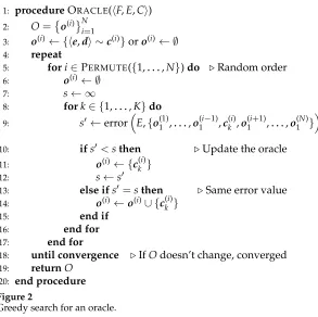
1: procedureORACLE(hF,E,Ci)

2: O=

o(i) N_i=1

3: o(i)← {he,di ∼c(i)}oro(i)← ∅

4: repeat

5: fori∈PERMUTE({1,. . .,N})do .Random order

6: o(i)← ∅

7: s← ∞

8: fork∈ {1,. . .,K}do

9: s0←errorE,{o(1)₁ ,. . .,o₁(i−1),c_k(i),o(₁i+1),. . .,o(₁N)}

10: ifs0<sthen .Update the oracle

11: o(i)← {c(_ki)}

12: s←s0

13: else ifs0=sthen .Same error value

14: o(i)←o(i)∪ {c(_ki)}

15: end if

16: end for

17: end for

18: until convergence .IfOdoesn’t change, converged

19: returnO 20: end procedure Figure 2

Greedy search for an oracle.

However, when using a corpus-level error function we need a slightly more sophisticated method, such as the greedy method of Venugopal and Vogel (2005). In this method (Figure 2), the oracle is first initialized either as an empty set or by randomly picking from the candidates. Next, we iterate randomly through the translation candidates inc(i)_{, try replacing the current oracle o}(i) _{with the candidate,}

and check the change in the error function (Line 9), and if the error decreases, replace the oracle with the tested candidate. This process is repeated until there is no change inO.

4.3 Selecting Oracles for Margin-Based Methods

to use in the update as follows (Chiang, Marton, and Resnik 2008; Chiang, Knight, and Wang 2009):

he¯(i), ¯d(i)i=arg max he,di∈c(i)

w>h(f(i),e,d)+err(e(i),e) (35)

he˙(i), ˙d(i)i=arg max he,di∈c(i)

w>h(f(i),e,d)−err(e(i),e) (36)

Thus, we can replaceheˆ(i), ˆd(i)iandhe∗(i),d∗(i)iwithhe¯(i), ¯d(i)iandhe˙(i), ˙d(i)i, resulting in a margin of

∆err(e(i), ˙e(i), ¯e(i))−w>∆h(f(i), ˙e(i), ˙d(i), ¯e(i), ¯d(i)) (37)

which is the largest margin in thek-best list. Explaining more intuitively, this criterion provides a bias towards selecting hypotheses with high error, making the learning algorithm work harder to correctly classify very bad hypotheses than it does for hy-potheses that are only slightly worse than the oracle. Inference methods that consider the loss as in Equations (35) and (36) are called loss-augmented inference (Taskar et al. 2005) methods, and can minimize losses with respect to the candidate with the largest violation. Gimpel and Smith (2012) take this a step further, defining a structured ramp loss that additionally considers Equations (28) and (29) within this framework.

5. Batch Methods

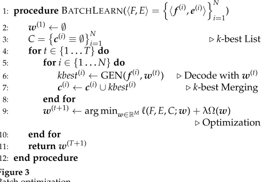
Now that we have explained the details of calculating loss functions used in ma-chine translation, we turn to the actual algorithms used in optimizing using these loss functions. In this section, we cover batch learning approaches to MT optimiza-tion. Batch learning works by considering the entire training data on every update of the parameters, in contrast to online learning (covered in the following section), which considers only part of the data at any one time. In standard approaches to batch learning, for every training example hf(i),e(i)i we enumerate every translation and derivation in the respective sets E(f(i)) and D(f(i)), and attempt to adjust the parameters so we can achieve the translations with the lowest error for the entire data.

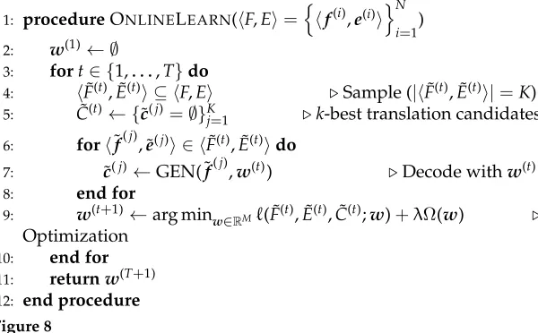
However, as mentioned previously, the entire space of derivations is too large to handle in practice. To resolve this problem, most batch learning algorithms for MT follow the general procedure shown in Figure 3, performing iterations that alternate between decoding and optimization (Och and Ney 2002). In line 6, GEN(f(i),w(t))= n

he(_ki),d_k(i)ioK

k=1 indicates that we use the current parametersw

(t)_{to perform decoding}

of sentencef(i), and obtain a subset of all derivations. For convenience, we will assume that this subset is expressed using ak-best listkbest(i), but it is also possible to use lattices or forests, as explained in Section 2.4.

1: procedureBATCHLEARN(hF,Ei=nhf(i),e(i)ioN

i=1)

2: w(1)← ∅

3: C=c(i)≡ ∅ N_i=1 .k-best List

4: fort∈ {1. . .T}do

5: fori∈ {1. . .N}do

6: kbest(i)←GEN(f(i),w(t)) .Decode withw(t)

7: c(i)←c(i)∪kbest(i) .k-best Merging

8: end for

9: w(t+1)←arg minw∈RM`(F,E,C;w)+λΩ(w)

.Optimization

10: end for

11: returnw(T+1) 12: end procedure Figure 3

Batch optimization.

errors in decoding means that we are not even guaranteed to find the highest-scoring hypotheses, this approximation is far from perfect. The effect of this approximation is particularly obvious if the lack of coverage of thek-best list is systematic. For example, if the hypotheses in thek-best list are all much too short, optimization may attempt to fix this by adjusting the parameters to heavily favor very long hypotheses, far overshooting the actual optimal parameters.7

As a way to alleviate the problems caused by this approximation, in line 7 we merge thek-best lists from multiple decoding iterations, finding a larger and more accurate set

Cof derivations. GivenCand the training datahF,Ei, we perform minimization of the Ω(w) regularized loss function`(·) and obtain new parametersw(t+1) (line 9). Gener-ation ofk-best lists and optimization is performed until a hard limit ofT iterations is reached, or until training has converged. In this setting, usually convergence is defined as any iteration in which the mergedk-best list does not change, or when the parameters wdo not change (Och 2003).

Within this batch optimization framework, the most critical challenge is to find an effective way to solve the optimization problem in line 9 of Figure 3. Section 5.1 describes methods for directly optimizing the error function. There are also methods for optimizing other losses such as those based on probabilistic models (Section 5.2), error margins (Section 5.3), ranking (Section 5.4), and risk (Section 5.5).

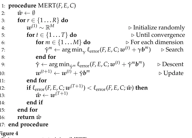
5.1 Error Minimization

5.1.1 Minimum Error Rate Training Overview.Minimum error rate training (MERT) (Och 2003) is one of the first, and is currently the most widely used, method for MT optimization, and focuses mainly on direct minimization of the error described in Section 3.1. Because error is not continuously differentiable, MERT uses optimization methods that do not require the calculation of a gradient, such as iterative line search

1: procedureMERT(F,E,C)

2: wˆ ← ∅

3: forr∈ {1. . .R}do

4: w(1)∼_RM _{.Initialize randomly}

5: fort∈ {1. . .T}do .Until convergence

6: form∈ {1. . .M}do .For each dimension

7: γˆm←arg minγ`error(F,E,C;w(t)+γbm) .Search

8: end for

9: γˆ ←arg min_γˆm`_error(F,E,C;w(t)+γˆmbm) .Descent 10: w(t+1)←w(t)+γˆbm .Update

11: end for

12: if`<sub>error</sub>(F,E,C;w(T+1))< `_error(F,E,C; ˆw)then

13: wˆ ←w(T+1)

14: end if

15: end for

16: returnwˆ

17: end procedure Figure 4

Minimum error rate training (MERT).

inspired byPowell’s method(Och 2003; Press et al. 2007), or theDownhill-Simplex method (Nelder-Mead method) (Press et al. 2007; Zens, Hasan, and Ney 2007; Zhao and Chen 2009).

The algorithm for MERT using line search is shown in Figure 4. Here, we assume that w and h(·) are M-dimensional, and bm is an M-dimensional vector where the

m-th element is 1 and the rest of the elements are zero. For theTiterations, we decide the dimension m of the feature vector (line 6), and for each possible weight vector w(j)+γbm choose the γ∈_Rthat minimizes `_error(·) using line search(line 7). Then, among theγfor each of theMsearch dimensions, we perform an update using ˆγthat affords the largest reduction in error (lines 9 and 10). This algorithm can be deemed a variety of steepest descent, which is a standard method used in most implemen-tations of MERT (Koehn et al. 2007). Another alternative is a variant of coordinate descent (e.g., Powell’s method), in which search and update is performed in each dimension.

One feature of MERT is that it is known to easily fall into local optima of the error function. Because of this, it is standard to chooseRstarting points (line 4), perform optimization starting at each of these starting points, and finally choose the ˆw that minimizes the loss from the weights acquired from each of the R random restarts. The R starting points are generally chosen so that one of the points is the best w from the previous iteration, and the remainingR−1 have each element ofwchosen randomly and uniformly from some interval, although it has also been shown that more intelligent choice of initial points can result in better final scores (Moore and Quirk 2008).

exact enumeration of which of theKcandidates inc(i)will be chosen for each value of

γ. Concretely, we define

arg max he,di∈c(i)

w(j)+γbm >h(f(i),e,d) (38)

=arg max he,di∈c(i)

w(j)>h(f(i),e,d)

| {z }

intercept

+γ·hm(f(i),e,d)

| {z }

slope

(39)

=arg max he,di∈c(i)

a(f(i),e,d)+ γ·b(f(i),e,d) (40)

where each hypothesishe,diinc(i)_{of Equation (40) is expressed as a line with intercept}

a(f(i),e,d)(=w(j)>_h(f(i)_{,e,d)) and slopeb(f}(i)_,e,d)(=h

m(f(i),e,d)) withγas a parame-ter. Equation (40) is a function that returns the translation candidate with the highest score. We can define a functiong(γ;f(i)) that corresponds to the score of this highest-scoring candidate as follows:

g(γ;f(i))= max he,di∈c(i)a(f

(i)_{,e,d)+γ·b(f}(i)_{,e,d) (41)}

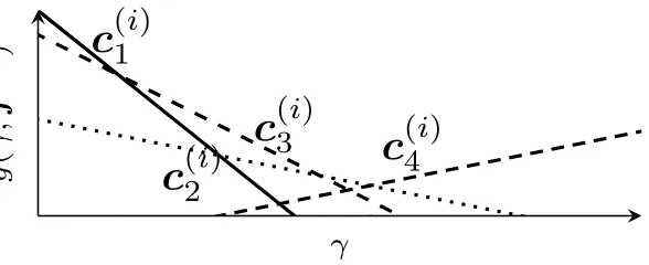
We can see that Equation (41) is apiecewise linearfunction (Papineni 1999; Och 2003), as at any given γ∈_R the translation candidate with the highest score a(·)+γ·b(·) will be selected, and this score corresponds to the line that is in the highest position at that particularγ. In Figure 5, we show an example with the following four translation candidates:

c(₁i): 2.5+γ·(−0.8),c(₂i): 1+γ·(−0.2)

c₃(i): 2+γ·(−0.5), c₄(i):−0.5+γ·0.2 (42)

If we setγto a very small value such as−∞, the candidate with the smallest slope, in this examplec(₁i), will be chosen. Furthermore, if we makeγgradually larger, we will

Figure 5

see thatc(₁i)continues to be the highest scoring candidate until we reach the intersection ofc(₁i)andc(₃i)at

2.5−2

(−0.5)−(−0.8) ≈1.667 (43)

after whichc(₃i)will be the highest scoring candidate. If we continue increasingγ, we will continue by selectingc₂(i)andc(₄i)starting at their corresponding intersections.

A function like Equation (41) that chooses the highest-scoring line for each span over γ is called an envelope, and can be used to compactly express the results we will obtain by rescoring c(i) _{according to a particularγ (Figure 6a). After finding the}

envelope, for each line that participates in the envelope, we can calculate the sufficient statistics necessary for calculating the loss`_error(·) and error error(·). For example, given the envelope in Figure 6a, Figure 6b is an example of the sentence-wise loss with respect toγ.

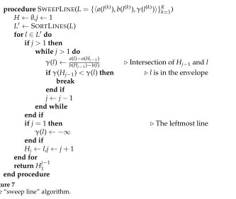
The envelope shown in Equation (41) can also be viewed as the problem of finding aconvex hullin computational geometry. A standard and efficient algorithm for finding a convex hull of multiple lines is the sweep line algorithm (Bentley and Ottmann 1979; Macherey et al. 2008) (see Figure 7). Here, we assume Lis a set of the lines corresponding to theKtranslation candidates inc(i), each linel∈Lis expressed as ha(l),b(l),γ(l)iwith intercepta(l)=a(f(i),e,d), and slopeb(l)=b(f(i),e,d). Furthermore, we defineγ(l) as an intersection initialized to−∞. SORTLINES(L) in Figure 3 sorts the lines in the order of their slopeb(l), and if two lineslk1 have the same slope,lk2 chooses the one with the larger intercepta(lk1)>a(lk2) and deletes the other. We next process the sorted set of linesL0(|L0| ≤K) in order of ascending slope (lines 4–18). If we assumeH

γ

g

(

γ

;

f

(

i

) )

(a) Envelope

γ `er

ror

(

·

)

(b) Loss

Figure 6

1: procedureSWEEPLINE(L={ha(l(k)),b(l(k)),γ(l(k))i}K k=1)

2: H← ∅,j←1

3: L0←SORTLINES(L)

4: forl∈L0do

5: ifj>1then

6: whilej>1do

7: γ(l)← a(l)−a(Hj−1)

b(Hj−1)−b(l) .Intersection ofHj−1andl

8: ifγ(Hj−1)< γ(l)then .lis in the envelope

9: break

10: end if

11: j←j−1

12: end while

13: end if

14: ifj=1then .The leftmost line

15: γ(l)← −∞

16: end if

17: Hj←l,j←j+1

18: end for

19: returnHj−₁ 1 20: end procedure Figure 7

The “sweep line” algorithm.

is the envelope expressed as the set of lines it contains, we find the line that intersects with line under consideration at the highest point (lines 6–12), and update the envelope

H. AsLcontains at mostKlines,H’s size is also at mostK.

Given a particular input sentence f(i), its set of translation candidates c(i), and the resulting envelopeH(i), we can also define the set of intersections between lines in the envelope asγ(₁i)<· · ·< γ_j(i)<· · ·< γ(i)

|H(i)_|. We also define∆`

(i)

j to be the change in the loss function that occurs when we move from one span [γ(_j−i)₁,γ(_ji)) to the next [γ(_ji),γ_j+(i)₁). If we first calculate the loss incurred when settingγ=−∞, then process the spans in increasing order, keeping track of the difference∆`(_ji) incurred at each span boundary, it is possible to efficiently calculate the loss curve over all spans ofγ.

5.1.3 MERT’s Weaknesses and Extensions.Although MERT is widely used as the standard optimization procedure for MT, it also has a number of weaknesses, and a number of extensions to the MERT framework have been proposed to resolve these problems.

The first weakness of MERT is therandomnessin the optimization process. Because each iteration of the training algorithm generally involves a number of random restarts, the results will generally change over multiple training runs, with the changes often being quite significant. Some research has shown that this randomness can be stabilized somewhat by improving the ability of the line-search algorithm to find a globally good solution by choosing random seeds more intelligently (Moore and Quirk 2008; Foster and Kuhn 2009) or by searching in directions that consider multiple features at once, instead of using the simple coordinate ascent as described in Figure 4 (Cer, Jurafsky, and Manning 2008). Orthogonally to actual improvement of the results, Clark et al. (2011) suggest that because randomness is a fundamental feature of MERT and other opti-mization algorithms for MT, it is better experimental practice to perform optiopti-mization multiple times, and report the resulting means and standard deviations over various optimization runs.

It is also possible to optimize the MERT objective using other optimization al-gorithms. For example, Suzuki, Duh, and Nagata (2011) present a method for using particle swarm optimization, a distributed algorithm where many “particles” are each associated with a parameter vector, and the particle updates its vector in a way such that it moves towards the current local and global optima. Another alternative optimization algorithm is Galley and Quirk’s (2011) method for usinglinear programmingto per-form search for optimal parameters over more than one dimension, or all dimensions at a single time. However, as MERT remains a fundamentally computationally hard problem, this method takes large amounts of time for larger training sets or feature spaces.

It should be noted that instability in MERT is not entirely due to the fact that search is random, but also due to the fact thatk-best lists are poor approximations of the whole space of possible translations. One way to improve this approximation is by performing MERT over an exponentially large number of hypotheses encoded in a translation lattice (Macherey et al. 2008) or hypergraph (Kumar et al. 2009). It is possible to perform MERT over these sorts of packed data structures by observing the fact that the envelopes used in MERT can be expressed as a semiring(Dyer 2010a; Sokolov and Yvon 2011), allowing for exact calculation of the full envelope for all hypotheses in a lattice or hypergraph using polynomial-time dynamic programming (theforward algorithmor inside algorithm, respectively). There has also been work to improve the accuracy of the

k-best approximation by either samplingk-best candidates from the translation lattice (Chatterjee and Cancedda 2010), or performing forced decoding to find derivations that achieve the reference translation, and adding them to thek-best list (Liang, Zhang, and Zhao 2012).