Munich Personal RePEc Archive
Panel Data Analysis with Stata Part 1
Fixed Effects and Random Effects
Models
Pillai N., Vijayamohanan
2016
Online at
https://mpra.ub.uni-muenchen.de/76869/
Panel Data Analysis with Stata
Part 1
Fixed Effects and Random Effects Models
Vijayamohanan Pillai N.
Centre for Development Studies,
Kerala, India.
2
Panel Data Analysis with Stata
Part 1
Fixed Effects and Random Effects Models
Abstract
3
Panel Data Analysis with Stata
Part 1
Fixed Effects and Random Effects Models
Panel Data Analysis: A Brief History
According to Marc Nerlove (2002), the fixed effects model of panel data techniques originated from the least squares methods in the astronomical work of Gauss (1809) and Legendre (1805) and the random effects or variance-components models, with an English astronomer George Biddell Airy, who published a monograph in 1861, in which he made explicit use of a variance components model for the analysis of astronomical panel data. The next stage is connected to R. A. Fisher, who coined the terms and developed the methods of variance and analysis of variance (Anova) in 1918; he elaborated both fixed effects and random effects models in Chapter 7: ‘Interclass Correlations and the Analysis of Variance’ and in Chapter 8: ‘Further applications of the Analysis of Variance’ of his 1925 work Statistical Methods for Research Workers. However, he was not much clear on the distinction between these two models. That had to wait till 1947, when Churchill Eisenhart came out with his ‘Survey’ that made clear the distinction between fixed effects and random effects models for the analysis of non-experimental versus experimental data. The random effects, mixed, and variance-components models in fact posed considerable computational problems for the statisticians. In 1953, CR Henderson developed the method-of-moments techniques for analysing random effects and mixed models; and in 1967, HO Hartley and JNK Rao devised the maximum likelihood (ML) methods for variance components models. The dynamic panel models started with the famous Balestra-Nerlove (1966) models. Panel data analysis grew into its maturity with the first conference on panel data econometrics in August 1977 in Paris, organized by Pascal Mazodier. Since then, the field has witnessed ever-expanding activities in both methodological and applied research.
4
Nomenclature
A cross sectional variable is denoted by xi, where i is a given case (household or industry or
nation; i = 1, 2, …, N), and a time series variable by xt, where t is a given time point (t = 1, 2, …,
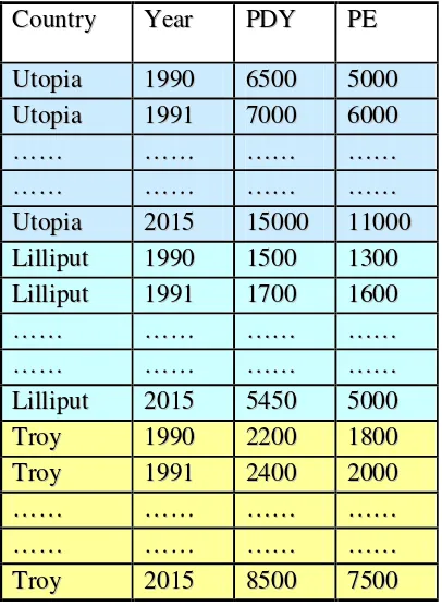
T). Hence a panel variable can be written as xit, for a given case at a particular time. A typical
[image:5.595.99.302.258.536.2]panel data set is given in Table 1 below, which describes the personal disposable income (PDY) and personal expenditure in three countries, Utopia, Lilliput and Troy over a period of time from 1990 – 2015.
Table 1: A Typical Panel Data Set
C
Coouunnttrryy YYeeaarr PPDDYY PPEE
U
Uttooppiiaa 11999900 66550000 55000000 U
Uttooppiiaa 11999911 77000000 66000000 …
……… ………… ………… ………… …
……… ………… ………… ………… U
Uttooppiiaa 22001155 1155000000 1111000000 L
Liilllliippuutt 11999900 11550000 11330000 L
Liilllliippuutt 11999911 11770000 11660000 …
……… ………… ………… ………… …
……… ………… ………… ………… L
Liilllliippuutt 22001155 55445500 55000000 T
Trrooyy 11999900 22220000 11880000 T
Trrooyy 11999911 22440000 22000000 …
……… ………… ………… ………… …
……… ………… ………… ………… T
Trrooyy 22001155 88550000 77550000
5
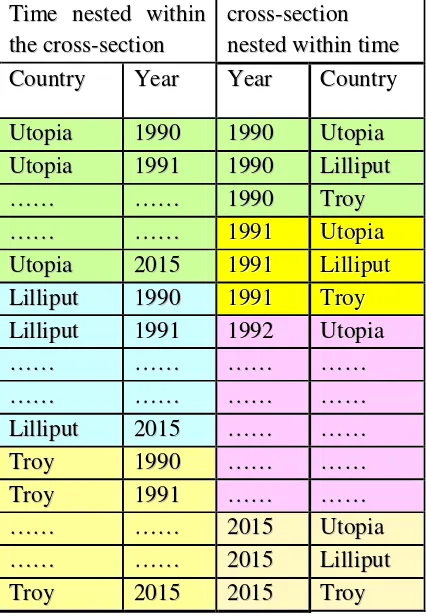
Table 2: Two Forms of Panel Configuration
T
Tiimmee nneesstteedd wwiitthhiinn
t
thheeccrroossss--sseeccttiioonn
c
crroossss--sseeccttiioonn n
neesstteeddwwiitthhiinnttiimmee
C
Coouunnttrryy YYeeaarr YYeeaarr CCoouunnttrryy
U
Uttooppiiaa 11999900 11999900 UUttooppiiaa U
Uttooppiiaa 11999911 11999900 LLiilllliippuutt …
……… ………… 11999900 TTrrooyy
…
……… ………… 19199911 UtUtooppiiaa
U
Uttooppiiaa 22001155 19199911 LiLilllliippuutt
L
Liilllliippuutt 11999900 19199911 TrTrooyy
L
Liilllliippuutt 11999911 11999922 UUttooppiiaa …
……… ………… ………… ………… …
……… ………… ………… ………… L
Liilllliippuutt 22001155 ………… ………… T
Trrooyy 11999900 ………… ………… T
Trrooyy 11999911 ………… ………… …
……… ………… 22001155 UUttooppiiaa …
……… ………… 22001155 LLiilllliippuutt T
Trrooyy 22001155 22001155 TTrrooyy
6
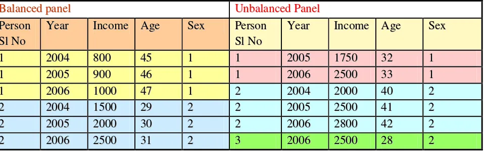
Table 3: Balanced and Unbalanced Panel
B
Baallaanncceeddppaanneell UUnnbbaallaanncceeddPPaanneell P
Peerrssoonn
S
SllNNoo Y
Yeeaarr IInnccoommee AAggee SSeexx PPeerrssoonn S
SllNNoo Y
Yeeaarr IInnccoommee AAggee SSeexx
1
1 22000044 880000 4455 11 11 22000055 11775500 3322 11 1
1 22000055 990000 4466 11 11 22000066 22550000 3333 11 1
1 22000066 11000000 4477 11 22 22000044 22000000 4400 22 2
2 22000044 11550000 2299 22 22 22000055 22550000 4411 22 2
2 22000055 22000000 3300 22 22 22000066 22880000 4422 22 2
2 22000066 22550000 3311 22 33 22000066 22550000 2288 22
We have two more models, depending upon the relative size of space and time, short and long panels. In a short panel, the number of time periods (T) is less than the number of cross section units (N), and in a long panel, T > N. Note that Table 1 above gives a long panel.
Advantages of Panel Data
Hsiao (2014) Baltagi (2008) and Andreß et al. (2013) list a number of advantages of using panel data, instead of pure cross-section or pure time series data.
The obvious benefit is in terms of obtaining a large sample, giving more degrees of freedom, more variability, more information and less multicollinearity among the variables. A panel has the advantage of having N cross-section and T time series observations, thus contributing a total of NT observations. Another advantage comes with a possibility of controlling for individual or time heterogeneity, which the pure cross-section or pure time series data cannot afford. Panel data also opens up a scope for dynamic analysis.
The main advantage of panel data comes from its solution to the difficulties involved in interpreting the regression coefficients in the framework of a cross-section only or time series only regeression, as we explain below.
Regression Analysis: Some Basics
Let us consider the following cross-sectional multiple regression with two explanatory variables, X1 and X2:
7 Note that X1 is said to be the covariate with respect to X2 and vice versa. Covariates act as
controlling factors for the variable under consideration. In the presence of the control variables, the regression coefficients βs are partial regression coefficients. Thus, β1 represents the marginal
effect of X1 on Y, keeping all other variables, here X2, constant. The latter part, that is, keeping X2
constant, means the marginal effect of X1 on Y is obtained after removing the linear effect of X2
from bothX1 and Y. A similar explanation goes for β2 also. Thus multiple regression facilitates to
obtain the pure marginal effects by including all the relevant covariates and thus controlling for their heterogeneity.
This we’ll discuss in a little detail below. We begin with the concept of partial correlation coefficient. Suppose we have three variables, X1, X2 and X3. The simple correlation coefficient r12
gives the degree of correlation between X1 and X2. It is possible that X3 may have an influence on
both X1 and X2. Hence a question comes up: Is an observed correlation between X1 and X2 merely
due to the influence of X3 on both? That is, is the correlation merely due to the common
influence of X3? Or, is there a net correlation between X1 and X2, over and above the correlation
due to the common influence of X3? It is this net correlation between X1 and X2 that the partial
correlation coefficient captures after removing the influence of X3 from each, and then estimating
the correlation between the unexplained residuals that remain. To prove this, we define the following:
Coefficients of correlation between X1 and X2, X1 and X3, and X2 and X3 are given by r12, r13, and
r23respectively, defined as
= ∑
∑ ∑ =
∑ , = ∑
∑ ∑ =
∑ and = ∑
∑ ∑ =
∑ . …(2’)
Note that the lower case letters, x1, x2, and x3, denote the respective variables in mean deviation
form; thus ( = − ), etc., and s1, s2, and s3 denote the standard deviations of the three
variables.
The common influence of X3 on both X1 and X2 may be modeled in terms of regressions of X1 on
X3, and X2 on X3, with b13as the slope of the regression of X1 on X3, given (in deviation form) by
8 Given these regressions, we can find the respective unexplained residuals. The residual from the regression of X1 on X3 (in deviation form) is e1.3 = x1 – b13 x3, and that from the regression of X2
on X3 is e2.3 = x2 – b23 x3.
Now the partial correlation between X1 and X2, net of the effect of X3, denoted by r12.3, is defined
as the correlation between these unexplained residuals and is given by . = ∑ . .
∑ . ∑ . . Note
that since the least-squares residuals have zero means, we need not write them in mean deviation form. We can directly estimate the two sets of residuals and then find out the correlation coefficient between them. However, the usual practice is to express them in terms of simple correlation coefficients. Using the definitions given above of the residuals and the regression coefficients, we have for the residuals: . = − , and . = − , and
hence, upon simplification, we get
. = ∑ . .
∑ . ∑ . = .
“This is the statistical equivalent of the economic theorist’s technique of impounding certain variables in a ceteris paribus clause.” (Johnston, 1972: 58). Thus the partial correlation coefficient between X1 and X2 is said to be obtained by keeping X3 constant. This idea is clear in
the above formula for the partial correlation coefficient as a net correlation between X1 and X2
after removing the influence of X3 from each.
When this idea is extended to multiple regression coefficients, we have the partial regression coefficients. Consider the regression equation in three variables, X1, X2 and X3:
X1i = α+ β2X2i + β3X3i + ui ; i = 1, 2, …, N. …. (3)
Since the estimated regression coefficients are partial ones, the equation can be written as:
X1i = a+ b12.3X2i + b13.2X3i , …. (4)
9 The estimate b12.3 is given by:
. =∑ ∑ ∑∑ ∑(∑ ∑) .
Now using the definitions of simple and partial correlation coefficients in (2) and (2’), we can rewrite the above as:
. = .
Why b12.3 is called a partial regression coefficient is now clear from the above definition: it is
obtained after removing the common influence of X3 from both X1 and X2.
Similarly, we have the estimate b13.2 given by:
. =∑ ∑ ∑∑ ∑(∑ ∑) = ,
obtained after removing the common influence of X2 from both X1 and X3.
Thus the fundamental idea in partial (correlation/regression) coefficient is estimating the net correlation between X1 and X2 after removing the influence of X3 from each, by computing the
correlation between the unexplained residuals that remain (after eliminating the influence of X3
from both X1 and X2). The classical text books describe this procedure as controlling for or
accounting for the effect of X3, or keeping that variable constant; whereas Tukey (in his classic
Exploratory Data Analysis, 1970, chap. 23) characterizes this as “adjusting for simultaneous linear change in the other predictor”, that is, X3. Above all these seeming semantic differences,
let us keep the underlying idea alive, while interpreting the regression coefficients.
Thus multiple regression facilitates controlling for the heterogeneity of the covariates.
10 impossible for this sample, as estimation breaks down because the number of observations is less than the number of parameters to be estimated.
The same problem haunts time series regression also. Consider the following time series multiple regression with two explanatory variables, X1 and X2:
Yt = α+ β1X1t + β2X2t + ut ; t = 1, 2, …, T. …. (2)
We have the same explanation for the marginal effects here also, and we know every time point in this system is different from one another. But we cannot account/control for this time heterogeneity by including time dummies, lest the estimation break down.
It is here panel data regression comes in with a solution. This we explain below.
The Panel Data Regression
Now combining (1) and (2), we get a pooled data set, which forms a panel data with the following panel regression:
Yit = α+ β1X1it + β2X2it + uit ; i = 1, 2, …, N; t = 1, 2, …, T. …. (3)
How do we account for the cross section and time heterogeneity in this model? This is done by using a two-way error component assumption for the disturbances, uit, with
uit = μi + λt + vit , … (4)
where μi represents the unobservable individual (cross section) heterogeneity, λt denotes the
unobservable time heterogeneity and vit is the remaining random error term. The first two
components (μi and λt) are also called within component and the last (vit), panel or between
component.
Now depending upon the assumptions about these error components, whether they are fixed or random, we have two types of models, fixed effects and random effects. If we assume that the μi
and λt are fixed parameters to be estimated and the random error term, vit, is identically and
independently distributed with zero mean and constant variance σv2 (homoscedasticity), that is, vit ∼ IID(0, σv2), then equation (3) gives a two-way fixed effects error component model or simply a
fixed effects model. On the other hand, if we assume that the μi and λt are random just like the
random error term, that is, μi, λt and vit are all identically and independently distributed with
zero mean and constant variance, or, μi ∼ IID(0, σμ2), λt ∼ IID(0, σλ2), and vit ∼ IID(0, σv2), with
11 equation (3) gives a two-way random effects error component model or simply a random effects model.
Instead of both the error components, μi and λt, if we consider any one component only at a time,
then we have a one-way error component model, fixed or random effects. Here the error term uit
in (3) will become:
uit = μi + vit , or, … (4’)
uit = λt + vit . … (4’’)
We can have one-way error component fixed or random effects model with the appropriate assumptions about the error components, that is, whether μi or λt is assumed to be fixed or
random.
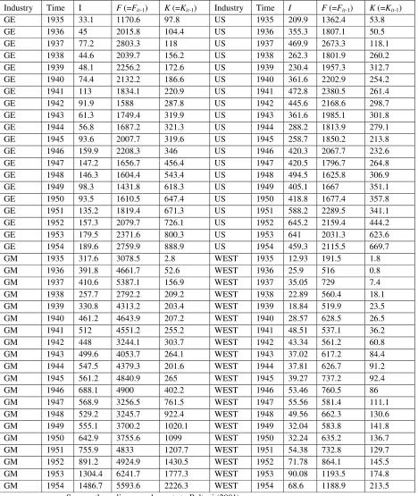
In the following we explain these models with regression results using a part of a data set from a famous study on investment theory by Yehuda Grunfeld (1958), who tried to analyse the effect of the (previous period) real value of the firm (F) and the (previous period) real capital stock (K) on real gross investment (I). For each variable, a positive effect is expected a priori. His original study included 10 US corporations for 20 years during 1935–1954. We consider only four companies – General Electric (GE), General Motor (GM), U.S. Steel (US), and Westinghouse (West) – for the whole period that gives 80 observations.
The investment model of Grunfeld (1958) is given as
Real gross investment (millions of dollars deflated by implicit price deflator of producers’ durable equipment), Iit = f(Fit-1, Kit-1),
where
Fit = Real value of the firm (share price times number of shares plus total book value of
debt; millions of dollars deflated by implicit price deflator of GNP), and
Kit = Real capital stock (accumulated sum of net additions to plant and equipment,
deflated by depreciation expense deflator – 10 year moving average of WPI of metals and metal products)
12
Table 4: The Panel Data That We Use
Industry Time I F (=Fit-1) K (=Kit-1) Industry Time I F (=Fit-1) K (=Kit-1)
GE 1935 33.1 1170.6 97.8 US 1935 209.9 1362.4 53.8 GE 1936 45 2015.8 104.4 US 1936 355.3 1807.1 50.5 GE 1937 77.2 2803.3 118 US 1937 469.9 2673.3 118.1 GE 1938 44.6 2039.7 156.2 US 1938 262.3 1801.9 260.2 GE 1939 48.1 2256.2 172.6 US 1939 230.4 1957.3 312.7 GE 1940 74.4 2132.2 186.6 US 1940 361.6 2202.9 254.2 GE 1941 113 1834.1 220.9 US 1941 472.8 2380.5 261.4 GE 1942 91.9 1588 287.8 US 1942 445.6 2168.6 298.7 GE 1943 61.3 1749.4 319.9 US 1943 361.6 1985.1 301.8 GE 1944 56.8 1687.2 321.3 US 1944 288.2 1813.9 279.1 GE 1945 93.6 2007.7 319.6 US 1945 258.7 1850.2 213.8 GE 1946 159.9 2208.3 346 US 1946 420.3 2067.7 232.6 GE 1947 147.2 1656.7 456.4 US 1947 420.5 1796.7 264.8 GE 1948 146.3 1604.4 543.4 US 1948 494.5 1625.8 306.9 GE 1949 98.3 1431.8 618.3 US 1949 405.1 1667 351.1 GE 1950 93.5 1610.5 647.4 US 1950 418.8 1677.4 357.8 GE 1951 135.2 1819.4 671.3 US 1951 588.2 2289.5 341.1 GE 1952 157.3 2079.7 726.1 US 1952 645.2 2159.4 444.2 GE 1953 179.5 2371.6 800.3 US 1953 641 2031.3 623.6 GE 1954 189.6 2759.9 888.9 US 1954 459.3 2115.5 669.7 GM 1935 317.6 3078.5 2.8 WEST 1935 12.93 191.5 1.8 GM 1936 391.8 4661.7 52.6 WEST 1936 25.9 516 0.8 GM 1937 410.6 5387.1 156.9 WEST 1937 35.05 729 7.4 GM 1938 257.7 2792.2 209.2 WEST 1938 22.89 560.4 18.1 GM 1939 330.8 4313.2 203.4 WEST 1939 18.84 519.9 23.5 GM 1940 461.2 4643.9 207.2 WEST 1940 28.57 628.5 26.5 GM 1941 512 4551.2 255.2 WEST 1941 48.51 537.1 36.2 GM 1942 448 3244.1 303.7 WEST 1942 43.34 561.2 60.8 GM 1943 499.6 4053.7 264.1 WEST 1943 37.02 617.2 84.4 GM 1944 547.5 4379.3 201.6 WEST 1944 37.81 626.7 91.2 GM 1945 561.2 4840.9 265 WEST 1945 39.27 737.2 92.4 GM 1946 688.1 4900 402.2 WEST 1946 53.46 760.5 86 GM 1947 568.9 3256.5 761.5 WEST 1947 55.56 581.4 111.1 GM 1948 529.2 3245.7 922.4 WEST 1948 49.56 662.3 130.6 GM 1949 555.1 3700.2 1020.1 WEST 1949 32.04 583.8 141.8 GM 1950 642.9 3755.6 1099 WEST 1950 32.24 635.2 136.7 GM 1951 755.9 4833 1207.7 WEST 1951 54.38 732.8 129.7 GM 1952 891.2 4924.9 1430.5 WEST 1952 71.78 864.1 145.5 GM 1953 1304.4 6241.7 1777.3 WEST 1953 90.08 1193.5 174.8 GM 1954 1486.7 5593.6 2226.3 WEST 1954 68.6 1188.9 213.5
Source: the online complements to Baltagi (2001):
13 Note that we have a balanced long panel (T = 20 > N = 4), where time is nested/stacked within cross section.
The model is generally written in matrix notation as:
yit = xit’β + αi+ uit ;
uit∼ IID(0, σu2); Cov(xit, uit) = 0;
where yit is the dependent variable, xit is the vector of regressors,
β is the vector of coefficients,
uit is the error term, independently and identically distributed with zero mean and σu2 variance;
and
αi = individual effects: captures effects of the i-th individual-specific variables that are constant
over time.
Panel Data with Stata
Unlike Gretl and EViews, Stata cannot receive data through dragging and dropping of excel file. We can open only a Stata file through the File → Open command. To enter data saved in Excel format, go to File → Import and select Excel spreadsheet. Next browse your Excel file and import the relevant sheet; mark “Import first row as variable names”. Or, in the command space, we can type:
. import excel "C:\Users\CDS 2\Desktop\Panel data Grunfeld.xlsx", sheet("Sheet2") firstrow
Note that we have a string variable “Industry” that Stata cannot identify; we have to generate a corresponding numerical variable by typing:
. encode Industry, gen(ind)
Alternatively, we can also type:
. egen ind = group(Industry)
We can see this new variable “ind” by typing:
14 Next we have to declare the data set to be a panel data. This we do by going to
Statistics → Longitudinal/panel data → Setup and utilities → Declare dataset to be panel data
Now set the panel id variable (“ind”) , time variable (“Time”) and the time unit (yearly).
Or, w can type:
. xtset ind Time, yearly
When we input this command, Stata will respond with the following:
panel variable: ind (strongly balanced)
time variable: Time, 1935 to 1954
delta: 1 year
Now that we have “xtset” the panel data, we can go for estimation.
Types of Panel Analytic Models:
We consider mainly three types of panel data analytic models: (1) constant coefficients (pooled regression) models, (2) fixed effects models, and (3) random effects models.
1. The Constant Coefficients (Pooled Regression) Model
If there is neither significant cross sectional nor significant temporal effect, we could pool all of the data and run an ordinary least squares (OLS) regression model with an intercept α and slope coefficients βs constant across companies and time:
Iit = α + β1Fit-1 + β2Kit-1 + uit ; uit∼ IIN(0, σu2); i = 1, 2, 3, 4; t = 1, 2, …, 20.
Note that for OLS regression in Stata, we need not “xtset” panel data; rather we can directly go to OLS regression through
15 Or, type
. regress I F K
or
. reg I F K
The regression output appears:
The Stata result includes some summary statistics and the estimates of regression coefficients. The upper left part reports an analysis-of-variance (ANOVA) table with sum of squares (SS), degrees of freedom (df), and mean sum of squares (MS). Thus we find the total sum of squares is 6410147.05, of which 4847828.25 is accounted for by the model and 1562318.8 is left unexplained (residual). Note that as the regression includes a constant, the total sum of squares, as well as the sum of squares due to the model, represents the sum of squares after removing the respective means. Also reported are the degrees of freedom, with total degrees of freedom of 79 (that is, 80 observations minus 1 for the mean removal), out of which the model accounts for 2 and the residual for 77. The mean sum of squares is obtained by dividing the sum of squares by the respective degrees of freedom.
The upper right part shows other summary statistics including the F-statistic and the R-squared. The F-statistic is derived from the ANOVA table as the ratio of the MS(Model) to the
MS(Residual), that is, F = !!/ #$%&'(
) *+ ,- !!/ #.'/0&12(. Thus F = 2423914.13 / 20289.8545 = 119.46,
with 2 numerator degrees of freedom and 77 denominator degrees of freedom. The F-statistic tests the joint null hypothesis that all the coefficients in the model excluding the constant are zero. The p-value associated with this F-statistic is the chance of observing an F-statistic that much large or larger, and is given as 0. Hence we strongly reject the null hypothesis and conclude that the model as a whole is highly significant.
16 Statistics → Postestimation → Tests → Test parameters
Or by typing
. testparm F K
The result is
This is exactly the same as the above.
The R-squared (R2) for the regression model represents the measure of goodness of fit or the coefficient of determination, obtained as the proportion of the model SS in total SS, that is, 4847828.25/ 6410147.05 = 0.7563, indicating that our model with two explanatory variables, F and K, accounts for (or explain) about 76% of the variation in investment, leaving 24% unexplained. The adjusted R2 (or R-bar-squared, R4 )is the R-squared adjusted for degrees of freedom, obtained as
R4 = 1 − !.'/0&12(
!6%72( = 1 −
) *+ ,- !!/ #.'/0&12(
8 9- !!/ #6%72( = 1 − (1 − R ) : #6%72( #.'/0&12(;.
Thus R4 = 1 − (1 − 0.7563) :AB
AA; = 0.7499. The root mean squared error, reported below the
adjusted R-squared as Root MSE. is the square root of the MS(Residual) in the ANOVA table, and equals √20289.8545 = 142.44. Note that this is the standard error (SE) of the residual.
17 The marginal effects of F and K are positive as expected, and highly significant, with K registering an effect nearly three times higher than that of F. The constant intercept also is significant.
Statistics – Postestimation – Reports and statistics
Unfortunately, we cannot have DW statistic for multiple panels:
2. The Fixed Effects Model
We have two models here: (i) Least Squares Dummy Variable model and (ii) Within-groups regression model.
2.1 The Fixed Effects (Least Squares Dummy Variable) Model:
If there is significant cross sectional or significant temporal effect, we cannot assume a constant intercept α for all the companies and years; rather we have to consider the one-way or two-way error components models; if the errors are assumed to be fixed, we have fixed effects model.
Iit = β1Fit-1 + β2Kit-1 + uit ; i = 1, 2, 3, 4; t = 1, 2, …, 20. … (5)
uit = μi + λt + vit , or uit = μi + vit , or, uit = λt + vit .
vit∼ IID(0, σv2);
Note that we have not explicitly included the fixed intercept α; it is subsumed under the error components, as will be clear later on.
18 describes every single dependent variable as an equation; for example, Iit = μi + vit , when we
consider only the company heterogeneity. This enables us to test, in the Anova framework, for the mean differences among the companies. One major problem with this (Anova) model is that it is not controlled for the relevant factors, for example, for the differences in F and K, such that the within-group (company) sum of squares will be an overestimate of the stochastic component in I, and the differences between company means will reflect not only the company effects but also the effects of differences in the values of the uncontrolled variables in different companies. When we include the covariates (F and K) to the Anova model to account for their effects, we get the Ancova model. Note that this interpretation is obtained when we consider Ancova as a regression within an Anova framework; on the other hand, when we consider Ancova as an Anova in a regression framework, the interpretation is in terms of assessing the marginal effects of the covariates after controlling for the effects of company differences. And this is precisely what we do in model (5). Note that the regression model gives us the marginal effects of quantitative variables, while the Anova model, those of qualitative factors; the Ancova model includes both quantitative and qualitative factors in a framework of controlling their effects.
Now the fixed effects model (5) can be discussed under two assumptions: (1) heterogeneous intercepts (μi ≠ μj, λt ≠ λs) and homogeneous slope (βi = βj; βt = βs), and (2) heterogeneous
intercepts and slopes (μi ≠ μj, λt ≠λs); (βi≠ βj; βt ≠βs). (Judge et al., 1985: Chapter 11, and
Hsiao, 1986: Chapter 1). In the former case, cross section and/or time heterogeneity applies only to intercepts, not to slopes; that is, we will have separate intercept for each company and/or for each year, but for all the companies and/or years, the slope will be common; for example, see the following figures, where we consider only the cross-section (company) heterogeneity:
The broken line ellipses in the above graphs represent the scatter plot of data points of each company over time, and the broken straight line in each scatter plot represent individual regression for each company. Note that the company intercepts vary, but the slopes are the same for all the companies (μi ≠ μj; βi = βj). Now if we pool the entire NT data points, the resultant
pooled regression is represented by the solid line, with altogether different intercept and slope that highlights the obvious consequence of pooling with biased estimates.
19
In general, we can consider the fixed effects panel data models with the following possible assumptions:
1. Slope coefficients constant but intercept varies over companies.
2. Slope coefficients constant but intercept varies over time.
3. Slope coefficients constant but intercept varies over companies and time.
4. All coefficients (intercept and slope) vary over companies.
5. All coefficients (intercept and slope) vary over time.
6. All coefficients (intercept and slope) vary over companies and time.
Last one = Random coefficients model. A random-coefficients model is a panel-data model in which group specific heterogeneity is introduced by assuming that each group has its own parameter vector, which is drawn from a population common to all panels.
Now consider our model:
Iit = β1Fit-1 + β2Kit-1 + uit ; i = 1, 2, 3, 4; t = 1, 2, …, 20. … (5)
uit = μi + λt + vit , or uit = μi + vit , or, uit = λt + vit .
vit∼ IID(0, σv2);
(i) Slope coefficients constant but intercept varies over companies.
20 Iit = β1Fit-1 + β2Kit-1 + uit ;
uit = μi + vit , vit∼ IID(0, σv2); i = 1, 2, 3, 4; t = 1, 2, …, 20.
Or,
Iit = μi + β1Fit-1 + β2Kit-1 + vit ; vit∼ IID(0, σv2); i = 1, 2, 3, 4; t = 1, 2, …, 20 … (6)
We also assume that the explanatory variables are independent of the error term.
In regression equation (6), we have for all the four companies separate intercepts, μi, which can
be estimated by including a dummy variable for each unit i in the model. A dummy variable or an indicator variable is a variable that takes on the values 1 and 0, where 1 means something is true (such as Industry is GE, sex is male, etc.). Thus our model may be written as
Iit = ΣμiDi+ β1Fit-1 + β2Kit-1 + vit ; vit∼ IID(0, σv2); i = 1, 2, 3, 4; t = 1, 2, …, 20 … (6)
Or,
Iit =μ1D1 +μ2D2 +μ3D3 +μ4D4 + β1Fit-1 + β2Kit-1 + vit;
where D1= 1 for GE; and zero otherwise.
D2= 1 for GM; and zero otherwise.
D3= 1 for US; and zero otherwise.
D4= 1 for WEST; and zero otherwise.
Note that the model we have started with does not have a constant intercept, and that is why we have included four dummies for the four companies. If the model does have a constant intercept, we need to include only three dummies, lest the model should fall in the ‘dummy variable trap’ of perfect multicollinearilty. In this case, our model will be
Iit =μ+μ2D2 +μ3D3 +μ4D4 + β1Fit-1 + β2Kit-1 + vit;
When D2 = D3 = D4 = 0, the model becomes
Iit =μ+ β1Fit-1 + β2Kit-1 + vit.
This is the model for the remaining company, GE. Hence, GE is said to be the ‘base company’, and μ , the constant intercept, serves as the intercept for GE.
If all the μs are statistically significant, we have differential intercepts, and our model thus accounts for cross section heterogeneity. For example, if μ and μ2 are significant, the intercept for
21 An advantage of this model is that all the parameters can be estimated by OLS. Hence this fixed effects model is also called least squares dummy variable (LSDV) Model. It is also known as covariance model, since the explanatory variables are covariates.
Now let us estimate this model in Stata by OLS. Note that we need not xtset our data for OLS estimation. But the LSDV estimation requires dummy variables for the four companies. In Stata this estimation we can do in two ways: one way is to create dummy variables in Stata using the
tabulate command and the generate( ) option, and use them directly in the regression command. Remember, we have already created a variable “ind” from the string variable “Industry”. Now typing
. tabulate ind, generate(D)
will generate four dummy variables, D1, D2, D3, and D4, corresponding to the four groups in “ind”, GE, GM, US and WEST. We can see these dummy variables by typing the command list
or going to Data → Data Editor → Data Editor (Edit).
Now we can have our OLS result with a constant and the last three dummy variables by typing:
. regress I F K D2 D3 D4
And the result is:
22 our ind variables is coded as GE = 1, GM = 2, US = 3 and WEST = 4. Then i.ind would cause Stata to create three 0/1 dummies. By default, the first category (in this case GE) is the reference (base) category, but we can change that, e.g. ib2.ind would make GM the reference category, or ib(last).ind would make the last category, WEST, as the base.
Now typing the following
. reg I F K i.ind
We get the same result as above.
The results on the marginal effects of F and K are similar to those from the pooled regression above; both the coefficients are positive and highly significant, with a very marginal fall in respect of F and a marginal increase in respect of K; now K has an effect a little more than three times higher than that of F.
The cross section (company) heterogeneity also is highly significant. Thus every company has its own significant intercept. The intercept for the base company, GE, is given by the constant intercept of the model, that is, – 242.758. And the intercepts of other companies are:
For GM = – 75.672 (= – 242.758 + 167.0862)
For US = 97.072 (= – 242.758 + 339.8296), and
23
Poolability Test (between Pooled Regression and FE Model)
Compared with our old pooled regression model, the new LSDV fixed effects model has a higher R2 value. Hence the question comes up: Which model is better? The pooled regression with constant slope and constant intercept or the LSDV fixed effects model with constant slope and variable intercept for companies? The question can be reframed also as: Can we assume that there is neither significant cross sectional nor significant temporal effect, and pool the data and run an OLS regression model with an intercept α and slope coefficients βs constant across companies and time? This is the poolability test.
Note that compared with the second (FE) model, the first one (pooled regression) is a restricted model; it imposes a common intercept on all companies: μ 2 = μ 3 = μ 4 = μ. Hence we have to do
the restricted F test given by
H = (IJK IK)/L ( IJK)/(M N)
where RUR2 = R2 of the unrestricted regression (second model) =0.9344;
RR2 = R2 of the restricted regression (first model) = 0.7563;
J = number of linear restrictions on the first model = 3;
k = number of parameters in the unrestricted regression = 6; and
n = NT = number of observations = 80.
Hence H =(O.B PP O.AQR )/
( O.B PP)/AP = 66.968, with a p-value equal to zero. Comparing this with F3,74 =
4.05787 at 1% right tail significance level, we find that the difference in the explanatory powers of the two models is highly significant and so conclude that the restricted regression (pooled regression) is invalid.
This poolability test we can do in Stata after the regression with the factor variable i.ind, by typing
. testparm i.ind
24 With this p-vale, we strongly reject the three null hypotheses of zero company effect.
Random Coefficient models (Another Poolability test)
In random-coefficients models, we wish to treat the parameter vector as a realization (in each panel) of a stochastic process. The Stata command xtrc fits the Swamy (1970) random-coefficients model, which is suitable for linear regression of panel data.
To take a first look at the assumption of parameter constancy, we go to
Statistics > Longitudinal/panel data > Random-coefficients regression by GLS
Or typing
25 The test included with the random-coefficients model also indicates that the assumption of parameter constancy is not valid for these data.
(ii) Slope coefficients constant but intercept varies over time.
Our second assumption is: no significant cross section differences, but significant temporal effects. That is, a linear regression model in which the intercept terms vary over time; so our model can be written as a one-way error component model:
Iit = β1Fit-1 + β2Kit-1 + uit ;
uit = λt + vit , vit∼ IID(0, σv2); i = 1, 2, 3, 4; t = 1, 2, …, 20.
Or,
Iit = λt + β1Fit-1 + β2Kit-1 + vit ; vit∼ IID(0, σv2); i = 1, 2, 3, 4; t = 1, 2, …, 20 … (7)
We also assume that the explanatory variables are independent of the error term.
In regression equation (7), we have for all the 20 years separate intercepts, λt, which can be
estimated by including a dummy variable for each year t in the model. Thus our model may be written as
Iit = Σλtdt+ β1Fit-1 + β2Kit-1 + vit ; vit∼ IID(0, σv2); i = 1, 2, 3, 4; t = 1, 2, …, 20 … (6)
Or,
Iit =λ1d1 +λ2d2 + …. + λ19d19 +λ20d20 + β1Fit-1 + β2Kit-1 + vit;
where d1 = 1 for year 1935; and zero otherwise, etc. up to d20 = 1 for year 1954; and zero
otherwise.
If the model is assumed to have a constant intercept, we need to include 19 time dummies, and our model will be
Iit =λ+λ2d2 + …. + λ19d19 +λ20d20 + β1Fit-1 + β2Kit-1 + vit;
Here the ‘base year’ is 1935, and λ , the constant intercept, serves as the intercept for that year.
If all the λs are statistically significant, we have differential intercepts, and our model thus accounts for temporal heterogeneity. For example, if λ and λ2 are significant, the intercept for
26 An advantage of this model is that all the parameters can be estimated by OLS. Hence this fixed effects model is also called least squares dummy variable (LSDV) Model. It is also known as covariance model, since the explanatory variables are covariates.
Now we turn to estimating this model in Stata by OLS. First we create time dummy variables in Stata using the tabulate command and the generate( ) option, as before:
. tabulate Time, generate(d)
This will generate 20 dummy variables, d1, d2, …, d19, and d20, corresponding to the 20 years from 1935 to 1954. We can see these dummy variables by typing the command list or going to Data → Data Editor → Data Editor (Edit).
Now we can have our OLS result with a constant and the last 19 dummy variables by typing:
. regress I F K d2 d3 d4 d5 d6 d7 d8 d9 d10 d11 d12 d13 d14 d15 d16 d17 d18 d19 d20
27 Now the same result we get using the factor variable i.Time, by typing the following:
29 Now Stata gives the poolability test result after the regression with the factor variable i.Time:
With this p-value, we cannot reject the F-test null of zero time effect.
Thus we have found that the company effects are statistically significant, but the time effects not. Does that mean our model is somehow misspecified? Let us now consider both company and time effects together.
(iii) Slope coefficients constant but intercept varies over companies and time.
This gives our two-way error components model:
Iit = β1Fit-1 + β2Kit-1 + uit ; i = 1, 2, 3, 4; t = 1, 2, …, 20. … (5)
uit = μi + λt + vit ,
vit∼ IID(0, σv2).
We also assume that the explanatory variables are independent of the error term.
With a constant intercept, our LSDV model is
30 with the same definitions for the dummy variables as above.
The constant intercept α, if significant, denotes the base company, GE, for the base year, 1935; if α and λ2 are significant, then α + λ2 gives the intercept for GE for the year 1936, and so on. The
Stata output for this model is:
The same output we get by typing
32 We have a little mixed results here; the dummy variable D2 associated with GM is significant
only at 10% level, and a few time dummies are significant at 5% or 10% level. The covariates and other two company dummies are highly significant. And the R2 value is higher at 0.9489. Compared with the pooled regression (with R2 = 0.7563), the F-test rejects in favour of our new LSDV model, but against out first LSDV model (with differential intercepts for companies, having R2 = 0.9344), this model fails the test with an increment of only 0.0145, indicating that the time effect is insignificant in general. We conclude that the investment function has not changed much over time, but changed over companies.
33 We reject the null: the intercepts are different across the companies and time in general.
34 Here we cannot the reject the null of zero time effects!
Then we do the F-test only for the company effects:
We do reject the null: the company effects are significant.
(iv) All coefficients (intercept and slope) vary over companies.
35 have to be included in the LSDV model in an interactive/multiplicative way, by multiplying each of the company dummies by each of the explanatory variables. Thus our extended LSDV model is:
Iit = μ + μ 2D2 + μ 3D3 + μ 4D4 + β1Fit-1 + β2Kit-1 + γ1 (D2 Fit-1)+ γ2 (D2Kit-1)
+ γ3 (D3 Fit-1)+ γ4 (D3 Kit-1) + γ5 (D4Fit-1)+ γ6 (D4 Kit-1)+ vit, …(8)
where the μs represent differential intercepts, and the βs and γs together give differential slope coefficients. The base company, as before, is GE, with a differential intercept of μ; β1 is the slope
coefficient of Fit-1 of the base company GE. If β1 and γ1 are statistically significant, then the
slope coefficient of Fit-1 of GM is given by (β1 + γ1), which is different from that of GE.
It is very difficult to specify the regression equation command using so many dummy variables in additive and multiplicative ways. Stata has certain easy ways to deal with this problem, using the factor variables and the cross operator #; the latter is used for interactions and product terms. However, note that when we use the cross operator along with the i. prefix with variables, Stata by default assumes that the variables on both the sides of the # operator are categorical and computes interaction terms accordingly. Hence we must use the i. prefix only with categorical variables. When we have a categorical variable (ind) along with a continuous variable (F or K), we must use the i. prefix with the categorical variable (i.ind) and c. prefix with the continuous variable (c.F or c.K). Thus the simple command i.ind#c.F or i.ind#c.K will give us an indication of the slope differential over the companies. Also note that c.F#c.F tells Stata to include the squared term of F (F2) in the model; we need not compute the variable separately.
Now the above model we estimate in Stata by typing
. reg I F K i.ind i.ind#c.F i.ind#c.K
36 We have the following results of F-tests:
37 We have some mixed results here. Investment is significantly related only to K (by the individual t-test), even though the F-test rejects the null of zero coefficients for both F and K in general. Thus the slope coefficient of the base company (GE) is significant only in respect of K. The slope differentials (γs) in respect of both F and K are significant only for GM and US, not for WEST, even though the F-test rejects the joint null (for all the three companies) strongly in respect of K and at a little more than 10% for F. Also note that all the company intercepts, including the constant, are insignificant.
(v) All coefficients (intercept and slope) vary over time.
This model assumes that all the slope coefficients as well as the intercept are variable over time; this means that all 20 years, from 1935 to 1954, have altogether different investment functions. This assumption is incorporated in our LSDV model by including the time dummies in both additive and interactive/multiplicative way. Thus our extended LSDV model is:
Iit =λ +λ2d2 +λ3d3 + … + λ20d20 + β1Fit-1 + β2Kit-1 + γ1 (d2 Fit-1)+ γ2 (d2Kit-1)
+ γ3 (d3 Fit-1)+ γ4 (d3 Kit-1) + … + γ37 (d20Fit-1)+ γ38 (d20 Kit-1)+ vit, …(9)
where the μs represent differential intercepts, and the βs and γs together give differential slope coefficients. The base year, as before, is 1935, with a differential intercept of λ; β1 is the slope
coefficient of Fit-1 of the base year, 1935. If β1 and γ1 are statistically significant, then the slope
coefficient of Fit-1 of 1936 is given by (β1 + γ1), which is different from that of the base year.
The Stata results using the indicator variables and cross operator are obtained by typing
. reg I F K i.Time i.Time#c.F i.Time#c.K
39
(vi) All coefficients (intercept and slope) vary over companies and time.
40 Iit =α + μ 2D2 + μ 3D3 + μ 4D4 + β1Fit-1 + β2Kit-1 + γ1 (D2 Fit-1) + γ2 (D2Kit-1) +
γ3 (D3 Fit-1) + γ4 (D3 Kit-1) + γ5 (D4Fit-1) + γ6 (D4 Kit-1) +
λ2d2 +λ3d3 + … + λ20d20 + β1Fit-1 + β2Kit-1 + δ1 (d2 Fit-1) + δ2 (d2Kit-1) +
δ3 (d3 Fit-1) + δ4 (d3 Kit-1) + … + δ37 (d20Fit-1) + δ38 (d20 Kit-1) + vit, …(10)
This model is estimated by typing
. reg I F K i.ind i.Time i.ind#c.F i.ind#c.K i.Time#c.F i.Time#c.K
43
2.2 The Fixed Effects (Within-groups Regression) Model
The main problem with the above fixed effects (LSDV) model, as is clear from the above, is that it hosts too many regressors; this makes the model numerically unattractive and infects it with the problems of multicollinearity. Moreover, as the number of regressors increases, the degrees of freedom fall, and the error variance rises, leading to Type 2 error in inference (not rejecting a false null hypothesis). Another problem is that this model is unable to identify the impact of time-invariant variables (such as sex, colour, ethnicity, education, which are invariant over time). Again, the assumption that the error term follows classical rules [that uit ~ N(0, σ2)] can go
wrong. For example, for a given period, it is possible that the error term for GM is correlated with the error term for, say, US or both US and WEST. If it so happens, we have to deal with it in terms of the seemingly unrelated regression (SURE) modelling aka Arnold Zellner (see Jan Kmenta 1986 Elements of Econometrics).
However, there is a simple way to estimate the fixed effects model without using dummy variables. Below we describe this.
Let us consider a simple one-way error components panel data model (with differential intercepts across individuals, which necessitate including dummy variables in estimation equation):
Yit = αi+ βXit + vit ; i = 1, 2, …, N; t = 1, 2, …, T. …(2.2.1)
vit∼ IID(0, σ2); Cov(Xit, vis) = 0; ∀t and s.
Averaging the regression equation over time gives
S.= T + V .+ W̅., …(2.2.2)
where S.= ∑ SY Y/Z, .= ∑Y Y/Z, and W̅.= ∑ WY Y/Z.
Now subtracting the first (2.2.1) equation from the second (2.2.2), we get
(SY− S.) =β( Y − .) + (WY − W̅.). …(2.2.3)
This deviations from means transformation is called Q transformation (Baltagi, 2008:15), which wipes out the differential intercepts. The OLS estimator for β from this transformed model is called within-groups FE estimator, or simply within estimator, as this estimator is based only on the variation within each company; this is exactly identical to the LSDV estimator. Since our panel model (2.2.1) is an Ancova model, the within estimator is also called covariance (CV)
estimator. The individual-specific intercepts are estimated unbiasedly as:
α
44 We can also have an OLS estimator for β from the mean equation (2.2.2); this estimate is known as the between-group FE estimator, or simply between estimator.
All the statistical packages report the within estimator for the FE model. Stata has an additional option to give the between estimator also.
Note that we have estimated all the LSDV fixed effects models by OLS, without setting our data to panel data mode, that is, without invoking the xtset command. Now once we have xtset our data (as we did earlier), we can have the Stata within-groups fixed effects estimation by going to
Statistics → Longitudinal/panel data → Linear models → Linear regression (FE, RE, PA, BE)
When the xtreg window appears, enter the dependent (I) and independent (F, K) variables and mark the model type as fixed effects. We can also type the command
. xtreg I F K, fe
The output is:
45 The xtreg command in Stata reports three R-squares, within, between and overall. Note that these reported R-squares do not share many of the properties of the OLS R2. The common properties of OLS R2 include the following:
(i) R2 is equal to the squared correlation between the dependent variable (Y) and its estimate (S\); and
(ii) R2 is equal to the proportion of the variation in Y explained by its estimate (S\); formally defined as R2 = Var(S\) / Var(Y), and lying in the range of 0 and 1. These variances are reported in the text books in terms of the sum of the squared deviations, or simply, sum of squares (SS): R2 = Explained (S\) SS / Total (Y) SS.
It is important to note that this identity of the definitions is a special property of the OLS estimates (see Johnston, 1972:34-35); in general, the squared correlation between a variable (Y) and its estimate (S\) need not be equal to the ratio of the variances, and the ratio of the variances need not be less than 1.
As already noted, the command xtreg, fe estimates (2.2.3) and (2.2.4) by OLS; hence its reported R2 within has all the properties of the usual R2. Other two R2s are correlations squared, corresponding to the between estimator equation and an overall equation with a constant intercept. Thus the usual R2 for our FE model is 0.8062, less than those for our earlier LSDV models. The overall R2 is similar to that of the pooled regression. The Stata reports a poolability test at the bottom of the results; Stata uses u_i for our μi; the F-test rejects the null of zero
company heterogeneity. Hence, between the pooled regression and FE model, we select the latter.
Stata also reports sigma_u, sigma_e, and rho; note that Stata’s u is our μ (intercept heterogeneity) and e stands for the random error term v in our one-way error component model. The FE model assumes that the μi (or Stata’s u_i) are formally fixed, having no distribution. Hence, we need
not bother about this estimate. However, in the random effects model, this estimate does natter.
Estimating Panel Effects
We can have the estimates of the individual (cross section or panel) effects in Stata; first estimate the FE model using the command
. xtreg I F K, fe
46 . predict IE, u
This will generate the individual effects (IE) that can be viewed in the Data Editor (Edit). Note that we can give any name , instead of IE, for example, the command
. predict pe, u
will give the same series with name pe (panel effects).
The Random Effects Model
Let us consider a simple one-way error components model;
Yit = α + βXit + uit ; i = 1, 2, …, N; t = 1, 2, …, T. …. (3)
uit = μi + vit , … (4)
In a FE model, the μis are assumed to be fixed. However, the main problem with the FE model is
its specification with too many parameters, resulting in heavy loss of degrees of freedom. This problem can be averted if the μis are assumed to be random; this gives us a random effects (RE)
model with
vit∼ IIN(0, σv2); μi∼ IID(0, σμ2);
Cov(vit, μi) = 0 Cov(vit, Xit) = 0 Cov(Xit, μi) = 0. ….(5)
Individual error components are not correlated with each other, and not autocorrelated across both cross-section and time series units.
The presence of α and μi in the equation means that the sample of our four companies are drawn
from the same population and have a common mean value for the intercept (α); the individual differences in the intercept values of each company are reflected in the error term μi.
Now let us consider the statistical properties of the composite error term uit = μi + vit:
Evidently, E(uit) = 0; and
47 Here we have a significant result. Note that if σμ2 = 0, then Var(uit) = σv2; and there is no
difference between the pooled regression model and the RE model; we can pool the data and run OLS. Hence the test on the null σμ2 = 0 can be taken as a poolability test in the context of pooled
regression vs. RE model. Such a test is available in Breusch-Pagan test, discussed below.
It is also evident that the variance of the composite error term [Var(uit) = σμ2 + σv2] is constant
and hence, the composite error term is homoscedastic for all i and t; but serially correlated over time only between the errors of the same company (unless σμ2 = 0). That is, under the assumptions in (5),
Cov(uit, ujs) = E[(μi + vit)(μj + vjs)] = σμ2 + σv2, for i =j, t = s [=Var(uit)]
= E(μi2) = σμ2, for i =j, t≠s (same company, over time)
= 0, otherwise.
And the correlation coefficient of uit and ujs is given by
ρ(uit, uis) = 1, for i =j, t = s [=Var(uit)/ Var(uit)]
= σμ2 /(σμ2 + σv2), for i =j, t≠s (same company, over time)
= 0, otherwise.
Thus the errors of each company are correlated over time; hence we call this correlation equi-correlation. The presence of such serial correlation makes the composite error term nonspherical, and the OLS estimation, inefficient.
In matrix notation, the OLS estimate of β is given by β\]^_ = ( ′ ) ′S, However, in the panel
context, it is often the case that the OLS assumptions about the spherical error will not be accurate, as shown above. If we knew the shape of the errors (that is, their variance-covariance matrix) we could simply use it to modify our data and then apply OLS to the transformed data; this would give the generalized least squares (GLS) estimates. If the shape of the errors is Ω (an NT x NT variance-covariance matrix of the errors), the estimate of β is given by β\`^_= ( ′ ) ′ S. In reality, often we might not know the shape of the errors and we could
only use an estimate of Ω; this would give the feasible generalized least squares (FGLS) estimates: β\a`^_ = ( ′b ) ′b S.
48 (cY−θS ) = (1 −θ)α+β( Y−θ ) + {(1 −θ) + (WY −θW̅ )},
where
θ= 1 − σf/(σf+ Zσ ).
This is given without proof in Hausman (1978:1262); also see Johnston (1984:402).
The term θ gives a measure of the relative sizes of the within and between component variances. We have the following results on the transformed quasi-deviation form model:
1. If θ = 1, the RE-estimator is identical with the FE-within estimator; this is possible when σv2 = 0, which means that every vit is zero, given E(vit) = 0; in this case the FE regression
will have an R2 of 1.
2. If θ = 0, the RE-estimator is identical with the pooled OLS-estimator; this is because, σμ2 = 0, which means that μi is always zero, given E(μi) = 0.
Normally, θwill lie between 0 and 1.
If Cov(Xit, μi) ≠ 0, the RE-estimator will be biased. The degree of the bias will depend on the size
of θ. If σμ2 is much larger than σv2, then θ will be close to 1, and the bias of the RE-estimator
will be low.
One major difficulty with RE estimator is that its small sample properties are unknown; it has only asymptotic properties.
Now let us turn to estimating the RE model for our data. Once we have xtset our data (as we did earlier), we can have the Stata random effects estimation by going to
Statistics → Longitudinal/panel data → Linear models → Linear regression (FE, RE, PA, BE)
When the xtreg window appears, enter the dependent (I) and independent (F, K) variables and mark the model type as GLS random-effects. We can also type the command
. xtreg I F K, re
49 Note that the marginal effects and intercept are almost equal to those of the FE-within model reported above; however, the intercept here is not at all significant. Also note that all the R2s are equal to those of the FE-within model. Since the RE estimator has only asymptotic properties, the F statistic for overall model significance is not reported here; rather, we have the results from a Wald chi-square test that indicates that the model as a whole is (all the coefficients taken jointly are) significant.
Stata obtains the result by assuming that the correlation of μi and the explanatory variables is
zero, or Cov(Xit, μi) = 0. This is reported as corr(u_i, X) = 0 (assumed).
Stata also reports sigma_u (our μ), sigma_e (our v), and rho. We have σμ = 150.78857 and σv =
75.401517 and rho = 0.79996932. Stata reports rho as “fraction of variance due to u_i”; remember our definition of this correlation: ρ = σμ2 /(σμ2 + σv2), the proportion of the variance of
μi in the total variance of the error components. Note that we do not have the estimate of theta,
used in the quasi-deviation in the results above, because we have not explicitly specified for it;
we can estimate it, using the formula θ= 1 − σf/(σf+ Zσ ), and the values of σμ =
150.78857 and σv = 75.401517 and T = 20 as theta = 0.8889, somewhat close to unity. If we
want the estimate of theta to be reported in the results, then we have to type
50 And the result is
We have seen that if σμ2 = 0, then the variance of the composite error term reduces to Var(uit) =
σv2; and there is no difference between the pooled regression model and the RE model; we can
pool the data and run OLS. Now given that σμ = 150.78857 here, we cannot do this. However, we can have a formal test in terms of Breusch-Pagan poolability test in the context of pooled regression vs. RE model by going to
Statistics → Longitudinal/panel data → Linear models → Lagrange multiplier test for random effects
or, by typing
. xttest0
51 We reject the null of σμ2 = 0; we cannot pool the data, but select the RE model.
We have earlier seen that in the context of pooled regression vs. FE model, we have favoured the FE model, and now in the context of pooled regression vs. RE model, we have selected the RE model. Now the question is: Which one is better, FE or RE?
FE- or RE-Modelling?
For most of the research problems, there is room to suspect that Cov(Xit, μi) ≠ 0. That means the
RE-estimator will be biased. Hence, it would be wiser to use the FE-estimator to get unbiased estimates. The RE-estimator, however, provides estimates for time-invariant covariates. Many studies would attempt to analyse the marginal effects of certain variables after accounting for the effects of sex, race, etc. This is possible only with the RE modeling. Suppose the cross section units are individual workers, and we want to study the workers’ earnings (Yi), including a
categorical variable for race (Zi) in the model:
Yit = β1Xit + β2Zi + uit ;
uit = μi + vit , vit∼ IID(0, σv2); i = 1, 2, …, N; t = 1, 2, …, T.
In the FE model, it would be impossible to estimate β2, because it would not be possible to
distinguish between the worker-specific constant term (μi) and the effect of the time-invariant
variable, race (Zi); the two would be perfectly multicollinear. Since RE accepts μi as a random
52 Judge, et al. (1988) propose the following simple rules:
1. If T is large and N small, there is little difference in the parameter estimates of FE and RE models. Hence computational convenience prefers FE model.
2. If N is large and T small, the two methods differ. If cross-sectional units in the sample are random drawings from a larger sample, RE model is appropriate; otherwise, FE model.
3. If the individual error component, μi, and one or more regressors are correlated, RE
estimators are biased and FE estimators unbiased
4. If N is large and T small, and if the assumptions of RE modeling hold, RE estimators are more efficient.
In most applications the assumption that Cov(xit, μi) = 0 may be wrong, and the RE-estimator
will be biased. “This is risking to throw away the big advantage of panel data only to be able to write a paper on "The determinants of Y"”. (Josef Brüderl, 2005: Panel Data Analysis).
However, we can have a test for RE vs. FE, in terms of the null hypothesis H0: E(uit| Xit) = 0.
Note that this null implies H0: E(μi | Xi) = 0. Hausman (1978) proposes to compare β\Ig and β\ag ,
both of which are consistent under the null H0: E(uit| Xit) = 0. In fact, β\ag is consistent whether
the null is true or not, whereas β\Ig is best linear unbiased estimator (BLUE), consistent and asymptotically efficient under the null, but is inconsistent when the null is false. Note that any test statistic for a mean difference comparison consists in the ratio of the difference between the statistics to its standard error, or the squared ratio in asymptotic cases. Thus a test statistic in our case can be based on the mean difference hi =β\Ig−β\ag; under the null, the probability limit of this value is: plim hi = 0, and Cov( β\Ig, hi) = 0. The variance of this mean difference is Var(hi) = Var(β\Ig) – Var(β\ag). Thus the test statistic for Hausman’s specification test is ℎ = hi′[lm (hi)] hi, where hi =β\
Ig−β\ag and Var(hi) = Var(β\Ig) – Var(β\ag), to test the null H0:
E(μi | Xi) = 0 against the alternative Ha: E(μi | Xi) ≠ 0. Under the null hypothesis, this statistic is
distributed asymptotically as central chi-squared, with k (= number of parameters) degrees of freedom.
Now we turn to conducting the Hausman test to see whether a fixed-effects or random effects model is more appropriate for the Grunfeld data that we consider. The procedure in Stata is as follows:
Estimate the FE model by typing
. xtreg I F K, fe
53 . estimates store fe
Then estimate the RE model by typing
. xtreg I F K, re
And do the Hausman test by typing
. hausman fe
The output is
The test fails to reject the null, as the p-value (Prob>chi2) is greater than 5%. Note that the Hausman test is a test of
H0: random effects would be consistent and efficient, versus
H1: random effects would be inconsistent.