Munich Personal RePEc Archive
Understanding intergenerational
economic mobility by decomposing joint
distributions
Richey, Jeremiah and Rosburg, Alicia
Kyungpook National University, University of Northern Iowa
19 July 2016
Online at
https://mpra.ub.uni-muenchen.de/72665/
Understanding Intergenerational Economic Mobility by Decomposing
Joint Distributions
Jeremiah Richey Kyungpook National University
Daegu, South Korea Phone: 82-053-950-7442
jarichey80@gmail.com
Alicia Rosburg 209 Curris Business Building
University of Northern Iowa Cedar Falls, Iowa 50614
Phone: (319)273-3263 Fax: (319)273-2922 alicia.rosburg@uni.edu
July 19, 2016
Abstract
We propose a simple and generalizable decomposition method to evaluate intergenerational economic mobility. The method decomposes the difference between the empirical parent-offspring joint distribution of incomes and a hypothetical independent parent-offspring joint distribution of incomes. The difference is attributed to (1) a portion due to a link between parental income and offspring characteristics (a com-position effect) and (2) a portion due to a link between parental income and the returns to characteristics (a structure effect). The method is based on the estimation of counterfactual joint distributions consis-tent with (actual and counterfactual) conditional distributions estimated via distributional regression and (actual and counterfactual) distributions of covariates. The counterfactual joint distributions are then caste into common measures of mobility found in the literature: intergenerational elasticities of incomes and their quantile regression counterparts, transition matrices, summary indices of transition matrices, and upward mobility probabilities. These counterfactual measures are used to assign portions of mea-sured (im)mobility to composition and structure effects. We apply the method to U.S. intergenerational economic mobility of white males born between 1957 and 1964. Across multiple mobility measures and using two different counterfactuals, we find that the composition effect (i.e., differences in the distribution of characteristics) generally accounts for about 60-70% of the measured mobility gap. Further, we find evidence of a safety-net effect of parental income which appears to be primarily compositional in nature.
JEL Classification: C14, C20, J31, J62
Key Words: intergenerational mobility, decomposition methods
1
Introduction
Kindled by the seminal papers of Becker and Tomes (1979, 1986), a large body of economics literature has sought to
understand the persistence of incomes across generations.1 Great strides have been made in understanding measure-ment issues and how they may bias results, and as a result, our understanding and empirical estimates of mobility
are much improved (B¨ohlmark and Lindquist, 2006; Haider and Solon, 2006; Nybom and Stuhler, 2015; Mazumder,
2005; Solon, 1999). The literature that seeks to understand this intergenerational link has focused primarily on
simple mean effects, such as the intergenerational elasticity of income (IGE) (Bj¨orklund et al, 2006; Blanden et al.,
2007; Bowles and Gintis, 2002; Cardaket al., 2013; Lefgrenet al., 2012; Liu and Zeng, 2009; Mayer and Lopoo, 2008;
Richey and Rosburg, 2016; Shea, 2000); mean effects are informative but provide a relatively limited view of mobility.
Two exceptions are Bhattacharya and Mazumder (2011), who estimate conditional directional mobility measures and
transition matrices, and Richey and Rosburg (2016), who decompose transition matrices and related indices. While
both studies are revealing and provide important additions to the literature, they have limitations that restrict their
generalizability.2 We propose a simple, generalizable estimation method that ‘decomposes’ the joint distribution of parental and offspring incomes into the portion due to a link between parental income and offspring characteristics
(a composition effect) and the portion due to a link between parental income and the returns to characteristics (a
structure effect).3 The decomposition is achieved by estimating a counterfactual joint distribution based on the
removal of one of these effects. This counterfactual joint distribution can then be used to analyze any measure of
(im)mobility and identify what portion is compositional or structural in nature.
The proposed method builds on the large body of decomposition literature which seeks to understand differences in
some outcome between groups. A prime example in labor economics is wage differences between men and women. The
method often used to investigate such differences is some variation of the Oaxaca-Blinder (OB) decomposition (Oaxaca
1974, Blinder 1973). While the traditional OB decomposition focuses on understanding simple mean differences, recent
literature has extended the traditional OB decomposition beyond simple mean comparisons to evaluate differences
between two groups across the full distribution and functions thereof (Chernozhukov et al., 2013; DiNardo et al.,
1996; Firpoet al., 2007; Machado and Mata, 2005; Roth, 2016). In some instances, however, the relevant question
pertains to an outcome that varies along a continuous group membership rather than binary group membership. In
particular, the literature on economic mobility seeks to understand to what degree and why offspring incomes vary
with parental incomes. In this case, the outcome (offspring income) varies along a continuous group membership
1Of course, interest in intergenerational income persistence predates these papers, especially in the field of sociology (see
Blau and Duncan 1967).
2Notably, the non-parametric procedure proposed by Bhattacharya and Mazumder (2011) is limited by the curse of
di-mensionality, and as a result, their application is limited to conditioning on a single covariate at a time. The decomposition approach by Richey and Rosburg (2016) relies on arbitrary segmentations of the population (e.g., parental income quartiles).
3The method proposed here can be characterized as a generalization of the Richey and Rosburg (2016) method. Richey
(parental income). While there is a large body of decomposition literature on binary groups, there is relatively less
work on ‘continuous group’ decompositions.4 Two notable exceptions are Ulrick (2012) and Nopo (2008) who evaluate
mean differences but allow ‘group membership’ to be continuous and compare means between ‘levels’ of this group
assignment; the procedure suggested here, which provides an aggregate decomposition of the full distribution of the
outcome of interest while allowing group membership to vary continuously, is a natural extension of their work.
The proposed method differs from traditional decompositions in that we do not ask what explains differences in
observed outcomes between two groups; rather, we ask what explains differences in theobserved joint distribution and a counterfactual joint distribution where offspring incomes are independent of parental income. To estimate
the counterfactual joint distribution that facilitates the decomposition, we begin by expressing the joint distribution
of parental and offspring incomes as a function of two components: (1) the distribution of offspring incomes
condi-tional on covariates and (2) the joint distribution of parental income and offspring covariates. These two components
incorporate the structure and composition effects. Our method simulates a hypothetical parental-offspring joint
dis-tribution that is a function of a counterfactual conditional disdis-tribution (of offspring incomes conditional on covariates)
and/or a counterfactual joint distribution (of parental income and offspring covariates). These components are easily
estimated, and with appropriately chosen components, we can identify which part of the mobility gap is compositional
or structural in nature.
To better understand the driving forces behind (im)mobility in the US, we apply the method to intergenerational
economic mobility of white males surveyed in the 1979 National Longitudinal Survey of Youth (NLSY). We base
our conditional CDF of incomes on an extended Mincer equation that includes education, experience, and cognitive
and non-cognitive measures. We decompose multiple mobility measures including standard IGEs, quantile regression
counterparts to the IGE, transition matrices, summary indices of transition matrices, and upward mobility
probabili-ties. Across the different mobility measures and evaluating two different counterfactuals, we find that the composition
effect (i.e., differences in the distribution of characteristics) generally accounts for about 60-70% of the mobility gap.
Further, we find the observed ‘safety-net’ effect of parental income is primarily compositional in nature.
4Richey and Rosburg (2016) circumvent this issue by discretizing the population along the transition matrix parental income
2
Method
2.1
Set-Up
Our goal is to understand the relationship between two variables - parental and offspring incomes. If yc is the
offspring’s (adult) income and yp is parental income, we are interested in why f(yc, yp) 6= f(yc)f(yp) ≡g(yc, yp).
That is, why do we not see an independent joint density, and if not, what are the mechanisms through which parental
income contribute to offspring income? Specifically, we wish to identify what part of the relationship is due to children
from different households having different characteristics (composition effect) and what part is due to similar children
from different households receiving different returns for those characteristics (structure effect).5
Mobility measures of interest are typically some function of the joint distribution, ν(f(yc, yp)), such as a
correla-tion, directional mobility measure or a summary index of a transition matrix. Therefore, we want to understand
ν(f(yc, yp))−ν(g(yc, yp)), which we define as the overall mobility gap:
∆ν
O =ν(f(yc, yp))−ν(g(yc, yp)) =νf−νg. (1)
Let us denote the actual joint density of (yc, yp) asfa|a, which can be expressed as:
fa|a=f(yc, yp) =
Z
f(yc|x:yp)f(yp, x)dx (2)
where f(yc|x : yp) is implicitly defined by a continuous set of wage structures yc = wyp(x, ǫ) with ǫ representing
the set of unobserved characteristics. Thex:yp notation in equation (2) denotes that parental income affects the
conditional distribution of offspring incomes through varying returns onxand also possibly throughǫ; see Fortinet
al. (2010) for a comprehensive discussion of identification in composition methods.6
In a similar manner, denote the independent joint densityg(yc, yp) asfi|i, which can be expressed as:
fi|i=g(yc, yp) =
Z
g(yc|x)g(yp, x)dx. (3)
The joint densityg(yp, x)≡f(yp)f(x) represents the hypothetical where the distribution of offspring characteristics
are independent of parental income. In addition, the conditional CDFg(yc|x) no longer allows for returns to depend
on parental income.
5This is the same goal as traditional decompositions on binary groups but with slightly different terminology due to our
focus on the continuous distribution.
6This aspect, in the traditional decomposition literature, is made explicit by defining separate conditional distributions
To conduct an aggregate decomposition of the mobility gap in equation (1), we need the counterfactual outcome that
would occur if one of the structure or composition connections were removed. As with decompositions in general, there
are two possible counterfactuals. In the gender wage gap literature, for example, one can choose the counterfactual
to be the outcomes of women if they were paid like men (but retained their characteristics) or the outcomes of men if
they were paid like women (but retained their characteristics). Equivalently, one could use the outcome of one group
if they had characteristics of the other group but retained their respective wage structures. In the context of parental
and offspring incomes, we do not have two (or even finite) distinct groups. Thus, while the general intuition remains,
our treatment will differ slightly.
First, consider a ‘structure’ counterfactual joint density denoted asfi|a:
fi|a=
Z
g(yc|x)f(yp, x)dx. (4)
This is the counterfactual density that would prevail if all children, regardless of parental incomes, received the
same returns for their productive characteristics (i.e., independent returns, actual characteristics). If we choose this
counterfactual and let ν(fi|a) = νi|a, we can derive the structure effect (∆νS,s) and composition effect (∆νX,s) as
follows:
∆νS,s=νf−νi|a (5)
∆νX,s=νi|a−νg, (6)
which, together, represent a decomposition of the mobility gap:
∆νO= ∆ ν S,s+ ∆
ν
X,s. (7)
Alternatively, consider a ‘composition’ counterfactual joint density denoted asfa|i:
fa|i=
Z
f(yc|x:yp)g(yp, x)dx (8)
This is the counterfactual that would prevail if all children, regardless of parental incomes, had the same distribution of
characteristics (i.e., actual returns, independent characteristics). If we choose this counterfactual and letν(fa|i) =νa|i,
the composition and structural effects can be expressed as:
∆νX,c=νf −νa|i (9)
which also represent a decomposition of the mobility gap:
∆ν O= ∆
ν S,c+ ∆
ν
X,c. (11)
The decomposition results will be well identified as long asignorability holds (Fortin et al., 2011).
Identifying Assumption - Ignorability: Let(yp, x, ǫ) have a joint distribution. For allxinX: ǫis independent
ofypgivenX =x.
The ignorability assumption assures that, conditional on observables, the distribution of unobservables are not
de-pendent on parental income.7 For example, if wealthier families had more ‘motivated’ or ‘unmotivated’ children
(unobserved), the decomposition will still be identified as along as the distribution of motivation is identical across
parental income when conditioned on observables.
2.2
Choice of
g
(
·
)
and Choice of Counterfactual
To estimate either counterfactual, we must choose an appropriateg(yc|x) org(yp, x) (specificallyf(x) for the latter).
In the traditional decomposition literature, this is usually the returns to, and the distribution of, characteristics
for one of the groups. An appealing choice for g(yp|x) is to extend the set up described in Neumark (1988) where
the ‘base’ returns to characteristics are assumed to be the returns that would exist if there where no differing
returns to characteristics across yp (i.e., the ‘non-discrimination world’). A simple choice would assume that the
returns in the ‘non-discriminatory’ world would be the unconditional set of returns actually observed in the market
(Neumark, 1988). Similarly, a simple choice forf(x) would be to assume the observed unconditional distribution
of characteristics would still prevail if the connection betweenypand xwere removed. Choosing the unconditional
distribution of characteristics would align with Nopo’s (2008) definition of the composition effect - the part due to
differences in characteristics between individuals and the ‘average’ individual.8
In standard (binary group) decompositions, the ‘choice ofg(·)’ is synonymous with ‘the choice of counterfactual’.
With the added complexity of decomposing the (continuous) joint distribution, these two choices are no longer
equivalent and we must choose both. Thus, we must also select which counterfactual (i.e., structural or composition)
to entertain. In general, they will lead to different results because the composition effect is ‘priced’ differently in the
7Ignorability is a less restrictive assumption thanindependence, which would require the unobservables to be independent
of the covariates. Only ignorability is needed for identification of the structure-composition decomposition.
8For most functionsν(·) of interest, however, the actual choice off(x) for f
i|i, and thus for the decomposition based on
the structure counterfactual, is a moot point; incorporating this effect simply moves us to the outcome whereyc andypare independent; many measures of interest such as correlations, transition matrices, summaries of these matrices, or transition probabilities are not affected by this choice. A similar argument holds for the choice of g(yc|x) in fi|i, and thus for the
two counterfactuals and the structure effect is ‘sized’ differently. For example, if we use the ‘structure counterfactual’
(fi|a), we first equate returns to characteristics across children regardless of parental income; this identifies and closes
the structure effect. The remaining gap - the composition effect - represents the portion explained by differences in
characteristics after returns for characteristics have been equated. As a result, differences in characteristics in the
composition effect are ‘priced’ at the equalized (non-discrimination) rate while differences in returns in the structure
effect are ‘sized’ by the actual (divergent) distributions of characteristics. Alternatively, if we take the ‘composition
counterfactual’ (fa|i), we first remove differences in characteristics between children from different parental income
levels; this identifies and closes the composition effect. The remaining gap - the structure effect - represents the
portion explained by children from different homes receiving different returns for characteristics after removing any
differences in characteristics. As a result, differences in characteristics in the composition effect are priced at the
actual (divergent) returns, while differences in returns in the structure effect are sized at the equalized distribution
of characteristics.
Thus, which counterfactual is more appropriate will depend on the research question of interest. For example, if
one is most interested in identifying the role of ‘privilege’ in a mobility gap, the structure counterfactual would
likely be more appropriate. However, if one is interested in how a policy aimed at equalizing education across all
households might shrink the mobility gap, then the composition decomposition would likely be more appropriate.
Not all questions or contexts will yield a clear counterfactual choice; in our empirical application, we choose to report
both and discuss why results differ if and when they do.
2.3
Estimation and Simulation
The decomposition rests on estimating the relevant counterfactual joint distribution. Estimation involves estimating
the conditional distribution (eitherf(yc|yp, x) org(yc|x)) and the joint distribution (eitherf(yp, x) org(yp, x)). Once
these components are estimated, the counterfactual density can be numerically approximated using the estimated
components for population components.
Conditional CDFs are easily estimated using the distributional regression approach suggested by Foresi and Peracchi
(1995); the foundation for this approach is a Probit model.9 The conditional CDF is estimated using multiple standard binary choice models where we vary the cut-off across a grid along the outcome space. Specifically, we repeatedly
estimateP r(yci≤y˜c|x) = Φ(xβy˜c) for ˜yc∈ YcwhereXis a vector of covariates (e.g., education, experience, cognitive,
and non-cognitive measures) andyc is log offspring income. Forf(yc|x:yp) parental income would be included in
the regressions and fully interacted with all covariates; in this aspect, this method can be seen as a direct extension
9Koenker and Bassett (1978) propose an alternative approach based on quantile regression. We refer readers interested in
of Ulrick’s (2012) method.10
For the joint distributionf(yp, x), we simply use the empirical distribution observed in the data. And forg(yp, x),
using the choice described in Section 2.2, we simply use the empirical distributions f(yp) and f(x) and construct
g(yp, x) asf(yp)f(x).11
Consider simulating the counterfactual joint densityfi|a. Once all of the above have been estimated, data simulation
follows a three step procedure that is very much in spirit with the procedure of Machado and Mata (2005):
1. Each observation is passed through the estimated conditional CDF - f(yc|x) - yielding a x-specific CDF of
incomes.
2. A set of random uniform variables (u∈[0,1]) are drawn, and a set ofyc’s are selected in accordance with the
estimated inverse CDF andu’s.12
3. Theyc’s are merged with our original (yp, x).
This yields the necessary data that would be generated by the conditional CDF and joint distributionf(yp, x). With
this, and similarly simulated counterfactual data sets, we can investigate any measure of mobility and ask what
explains the observed mobility gap.
3
Measuring Mobility
Alternative measures of mobility found in the literature represent different ways to summarize or capture some aspect
of the joint parent-offspring distribution of incomes. Thus, once the counterfactual joint densities have been estimated,
we can investigate the role of structural and compositional effects for any mobility measure of interest. Here, we
provide a brief overview of several commonly used measures: IGE, quantile counterparts to the IGE, transition
matrices, summary indices of transition matrices, and upward mobility probabilities.
10In particular, see equation (12) in Ulrick (2012). 11This is achieved by randomizingy
pacross ourX data.
12The size of the setuwill depend on the actual data at hand. For our application with sample sizen∼= 1,400, we use 200
3.1
Intergenerational Elasticity of Income
Much of the economic mobility literature models intergenerational mobility by regressing log earnings of a child
[ln(yc)] onto log parental earnings [ln(yp)], or:
ln(yc) =α+βln(yp) +ǫ. (12)
The value β is the IGE and (1−β) is a measure of intergenerational economic mobility. This simple relationship
is the workhorse of much of the existing literature on economic mobility. By comparing the observed (actual) IGE
with the IGE for our counterfactual joint density, we can ascertain what portion of the observed IGE is structural or
compositional in nature.
While the standard IGE approach (equation 12) tells us how the conditional mean of offspring income varies with
parental income, it is often informative to look beyond the simple mean. Therefore, a natural extension to the basic
IGE is through quantile regression. The goal of quantile regression, first introduced by Koenker and Bassatt (1979),
is to identify the effect of an explanatory variable on different points of the conditional distribution of the independent
variable. For example, previous results for the U.S. have shown larger IGE effects at the lower end of the income
distribution, which may reflect parental income acting as a safety net (Eide and Showalter, 1999). Our method allows
us to investigate not only how the relationship varies across the distribution but also what mechanism (compositional
or structural) drives the relationship across the distribution. Specifically, we model the conditional (τ) quantile of
offspring log income as:
Qln(yc)|ln(yp)(τ) =ατ+βτln(yp) (13)
whereτ is the quantile of interest such as the median, 25th percentile, or 75th percentile. The coefficient vectorβτ
will, in general, differ for each quantile. For example, the effect of parental earnings on the 25th percentile of the
conditional distribution of children’s earnings will likely differ from its effect on the median or on the 75th percentile.
Our decomposition method will identify the portion of eachβτ that is structural or compositional in nature.
As noted, the main shortcoming of the basic IGE is that it focuses on simple mean effects, and therefore, it may mask
interesting details in economic mobility across the distribution (Black and Devereux, 2011). Quantile regressions can
partially overcome this shortcoming by evaluating different quantiles of interest. An alternative and common way to
3.2
Transition Matrices and Related Indices
A transition matrix depicts the probability a child will have adult earnings (yc) in a specific income bracket given
parental income (yp) was in a certain income bracket. More specifically, let there bem income brackets (defined
as equal percentile groups) with boundaries 0 < ζ1 < ζ2 < ... < ζm−1 < ∞ for the parental distribution and
0 < ξ1 < ξ2 < ... < ξm−1 < ∞ for the children’s distribution. A transition matrix (P) is am×m matrix with
elementspij that represent the conditional probability that a child is in income bracketjgiven his/her parents were
in income bracketior
pij=
P r(ζi−1≤yp< ζiandξj−1≤yc< ξj)
P r(ζi−1≤yp< ζi)
.
Transition matrix can also be summarized through mobility indices, M(P), which map the transition matrix P
into a scalar value (Formbyet al., 2004). Because there is not a consensus on how mobility should be measured, a
number of mobility indices have been proposed.13 Each summary index reflects a different way to measure mobility,
and therefore, researchers have a degree of discretion in how they summarize the transition matrix. While our
decomposition approach extends to any of these proposed summary indices, we consider three indices commonly used
in the literature: M1 measures the average probability individuals leave their parent’s income bracket,M2is based on
the second largest eigenvalue (λ2) of the mobility matrix and can be interpreted as a correlation between parental and
offspring’s income group, andM3 is based on the average number of income groups crossed by individuals (Formby
et al., 2004).
M1=
(m−Pmi=1pii)
m ; M2= 1− |λ2|; M3=
m
X
i=1
m
X
j=1
πipij|i−j|. (14)
Richey and Rosburg (2016) propose a method to decompose transition matrices and related indices. Their procedure
discretizes the distribution of parental incomes into income brackets, performs multiple decompositions on these
groups, and then recasts them into transition matrices. The procedure proposed here avoids multiple decompositions
by groups and thus allows greater flexibility. Bhattacharya and Mazumder (2011) also investigate transition matrices,
but their work is confined to conditional transition probabilities rather than decomposing the transition matrix.
Moreover, their method is hindered by the curse of dimensionality which limits their investigation to conditioning on
one covariate at a time.
While transition matrices provide added information over IGE measures, their main drawback is dependence on
arbi-trary cut-offs in the distribution (Bhattacharya and Mazumder, 2011). To overcome this shortcoming, Bhattacharya
and Mazumder suggest directional mobility measures based on relative income positions rather than arbitrary
thresh-old bounds.
13See Maasoumi (1998) or Checchiet al. (1999) for relatively comprehensive overviews of summary mobility measures and
3.3
Directional Mobility
LetFc(y
c) andFp(yp) be child’s and parent’s marginal CDF of income and define an upward mobility measure based
on some ‘distance’τ (i.e., the degree to which the child moves above their parents rank) and some parental rank s
to be14:
ν(τ, s) =P r[Fc(yc)−Fp(yp)> τ|F(yp)≤s]. (15)
A key advantage of upward mobility measures over transition matrices is thatν(τ, s) captures the effect of children
moving beyond their parental ranks (or whatever τ is chosen) even if they do not cross some arbitrary quantile
threshold. For example, consider a quartile transition matrix and a son who moves up 10 percentile points relative
to his parents. If the son’s parents were in the 10th percentile of the income distribution and the son is in the
20th percentile, his movement would not contribute to ‘mobility’ as measured by the transition matrix because he is
still in the bottom quartile. But, if instead, the son’s parent were in the 20th percentile and the son is in the 30th
percentile, the transition matrix would capture this ‘mobility’ since the son crossed the 25% threshold. The benefit
of the upward mobility measure is that it captures both of these movements as a 10% increase in relative income
positions.
4
Data
The data for our analysis is the 1979 National Longitudinal Survey of Youth (NLSY79). The NLSY79 is a panel
survey of youths aged 14-22 in 1979. It includes a cross-sectional representative survey (n = 6,111), an over sample
of minorities and poor whites (n = 5,295), and a sample of military respondents (n = 1,280).15 We use only the cross-sectional representative survey.
We limit the sample to white males who reported living with a parent for at least two of the first three years of the
survey and with reported parental income for those years.16 A key variable of interest is parental status based on
the parents’ (average) income.17 The outcome of interest is the individual’s economic status based on their average
reported wage and salary income between 1996 and 1998. All incomes are deflated to 1982-1984 dollars using the
CPI.
14A downward mobility measure can be defined in an analogous fashion.
15The over sample of military and poor whites were discontinued in 1984 and 1990, respectively
16Parental income is identified through a comparison of total household income and respondent’s income. We exclude
individuals who lived with a spouse or child during these years.
17Measurement error in parental income is a common concern in the mobility literature. While recent research indicates that
The sample is further limited to individuals not enrolled in school over the period of interest and with available
Armed Forces Qualifying Test (AFQT) scores. The final sample includes 1,405 individuals with a mean age of 33.6
during our outcome years of interest (1996-1998).18 Table 1 provides summary statistics.
[Table 1 about here]
The variables we include in our decomposition are based on an extended Mincer equation. The traditional Mincer
equation includes education, experience, and experience squared (Mincer, 1974). We extend this basic model to
include other variables that have been related to income determination. In particular, we include a measure of
cognitive ability (AFQT) and three measures of non-cognitive ability (Esteem,Rotter, andPerlin).
The NLSY79 does not provide a direct measure of experience. Therefore, we construct a measure of ‘full time
equivalent’ (FTE) years of experience using the weekly array of hours worked.19 One FTE year of experience is assumed to equal 52 weeks times 40 hours (hours worked are top coded to 40). A few older individuals in our sample
completed their education prior to the beginning of the survey and therefore were already working during the first
round of interviews in 1979. Without information on previous work experience for these individuals, we construct the
following ‘pre-survey’ estimate of FTE years (F T E<79) based on age, years of schooling, and FTE years of experience
earned in the initial survey year: F T E<79= (Age79−Years of Schooling79−6)·F T E79. We then add the pre-survey
FTE years to the (observed) survey FTE years.
The measure of ability used in our analysis is Armed Forces Qualifying Test scores (AFQT). Since different individuals
took the test at different ages, the measure used is from an equi-percentile mapping used across age groups to create
age-consistent scores (Altonjiet al., 2012). The use of AFQT scores as a measure of ability warrants a brief discussion.
Some argue AFQT scores are proxies for IQ scores while others draw serious doubts to this interpretation (Ashenfelter
and Rouse, 2000). Others question what it is exactly IQ scores measure noting large changes in IQ scores over time
(Flynn, 2004). Therefore, we simply interpret AFQT scores as some combination of innate ability and accumulated
human capital as a youth that is valued in the labor market. However, for ease of expression, we will refer to AFQT
scores as our measure of ‘cognitive ability.’
We use three measures for non-cognitive ability. First, we use information from the Rosenberg Self-Esteem Scale
(1965). The Rosenberg Self-Esteem Scale contains 10 statements on self-approval and disapproval; we use a summary
measure of the individual’s responses to these 10 statements (Esteem). Second, we use a summary measure from the
Rotter-Locus of Control Scale (Rotter) which measures the “extent to which individuals believe they have control
18The literature on intergenerational mobility has identified the possibility of life-cycle biases is estimates depending on age
at which children are surveyed (B¨ohlmark and Lindquist, 2006; Haider and Solon, 2006; Nybom and Stuhler, 2015). However, this literature seems to indicate such biases are minimized or eliminated when youths reach their mid-30s.
over their lives through self-motivation or self-determination (internal control) as opposed to the extent that the
environment (that is, chance, fate, luck) controls their lives (external control)” (BLS, 2015). Rotter and Esteem
were measured in the first two rounds of the survey (1979 and 1980, respectively). Therefore, the third measure we
include is the Perlin Mastery Scale measured in 1992 when respondents were in their late 20s or early 30s. The Perlin
Mastery Scale measures the extent to which individuals “perceive themselves in control of forces that significantly
impact their lives” (BLS, 2015).
Educational attainment is measured as years of schooling and the endogenous nature of education in explaining
incomes is well documented. However, as long as the appropriate conditions hold (ignorability), this is not a concern
for theaggregatedecomposition.
5
Results
First, we consider the standard IGE results reported in column 1 of Table 2. The total mobility gap is 32.35.
Using the structure counterfactual, the structure effect accounts for a little over one-third of the gap (35%) while
the composition effect accounts for the other two-thirds (top panel, column 1). These results remain essentially
unchanged when we use the composition counterfactual instead (bottom panel). Together, these results suggest that
approximately 65% of the estimated IGE mobility gap is due to differences in characteristics between children from
different households, while the remaining gap is due to differences in returns to these characteristics. While the
structure effect is commonly interpreted as a measure of discrimination in traditional decomposition settings, Richey
and Rosburg (2016) argue that a more fitting interpretation in this context is some form of (loosely-termed) ‘privilege’
such as parental connections, parental knowledge/awareness of job market and education opportunities or perhaps
greater financial flexibility to facilitate job search. All of these would appear to the econometrician as higher returns
to similar productive characteristics.
The quantile IGE results in Table 2 reveal larger effects in the lower quantiles than upper quantiles, consistent with
the pattern reported by Eide and Showalter (1999). In particular, the total effect in the 10th quantile (52.42; column
2) is nearly double the effect in the 75th and 90th quantiles (27.23 and 27.34; columns 5 and 6). These results suggest
that parental income has a strong safety-net effect. Further, decomposition results suggest that this safety-net effect is
primarily compositional in nature. The composition effect explains about 50% of the total gap in the upper quantiles
but around 70% in the lower quantiles.
Tables 3 and 4 provide decomposed transition matrices using the structure and composition counterfactuals,
whose parent’s were in the bottom income quartile also ends up in the bottom quartile of his generation’s income
distribution. The total mobility gap of 14.49 (row 1, column 1) indicates that this probability is 14.49 percent higher
for sons in our sample compared to a transition matrix where offspring incomes are independent of parental income.
The decompositions indicate that the composition effect accounts for about 65% of this difference, with the structure
effect accounting for only about 35%. Similarly, when looking at what explains the relative absence of children from
the wealthiest homes from the bottom quartile of their income distribution (-12.22 in row 4, column 1), the
com-position effect accounts for about 70% and the structure effect accounting for the remaining 30%, regardless of the
counterfactual used. These results align with the quantile IGE results in that the composition effect is the primary
driver of the safety-net effect of parental income. However, when looking at what explains children from the poorest
homes being relatively absent from the top quartile of their income distribution (-9.66 in row 1, column 4), the results
diverge for the two decompositions. The composition effect explains 61% of this gap using the structure
counterfac-tual but only 29% of the gap using the composition counterfaccounterfac-tual. Similarly, when looking at what explains the
over-representation of children from top quartile income households in the top quartile of their income distribution
(17.33 in row 4, column 4), we get different results using the two counterfactuals. Using the structure counterfactual
assigns a 50-50 split between the composition and structure effect, while using the composition counterfactual assigns
a majority of the gap (62%) to the composition effect.
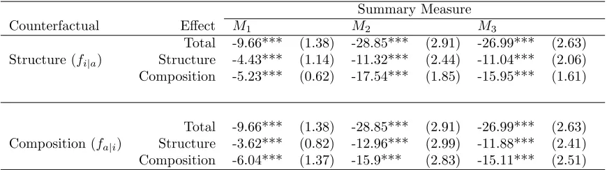
The transition matrix decomposition provides interesting detail regarding differences in mobility at different points
across the distribution, but it can be cumbersome to evaluate. Summary indices are a common and convenient way
to summarize a transition matrix through a single value. Table 5 provides decompositions of the three summary
indices defined in section 2.1. Looking at M1, a measure associated with the trace of the transition matrix, the
decomposition using the structure counterfactual weights the structure and composition effects almost evenly (46%
and 54%) whereas the decomposition using the composition counterfactual puts more weight (63%) on the composition
effect. Conversely, forM2, the composition effect is slightly larger (61%) with the structure counterfactual relative
to the decomposition using the composition counterfactual (55%). The third summary index,M3, yields very similar
splits between the composition and structure effect - the composition effect accounts for a little less than 60% of the
mobility gap and the structure effect a little over 40%. One shortcoming of transition matrices and related summary
indices is that they depend on arbitrary segmentation of the population (e.g., results in Tables 3-5 are based on a
4-by-4 quartile transition matrix). Nonetheless, theM2 andM3 measures appear fairly consistent to the size of the
transition matrix. Varying the matrix from 4-by-4 to 20-by-20, the structure effect for both M2 and M3 remains
fairly consistent at 35-40% of the measured mobility gap. TheM1 decomposition is more dependent on the size of
the matrix; the structure effect ranges between 35 and 60% of the total gap depending on matrix size. However,M1
is based only on the trace of the matrix, and therefore is the most limited of the three summary measures considered.
Given the concerns regarding arbitrary segmentation in the transition matrix, our final set of decompositions evaluates
decomposition is fairly consistent across all probabilities with the composition effect accounting for about two-thirds
of the mobility gap. The composition-structure split is less consistent with the composition counterfactual (Table 7).
In the third panel (τ= 0.2), the composition-structure split hovers around 2/3−1/3, which is similar to the structure
counterfactual results. However, as we lowerτto 0.1 in the second panel and to 0 in the first panel, the structure effect
shrinks such that the composition effect explains most of the measured mobility gap (especially at the lower levels of
s). These results suggest that the reason we see less upward mobility ofanysize in our observed sample relative to
the hypothetical case where offspring incomes are independent of parental income is primarily due to children from
different households having different characteristics. But, as we start to ask about larger upward movements, the
structure effect (i.e., differences in returns to these characteristics) begins to be part of the explanation.
6
Conclusion
A wealth of research over the past few decades has improved our understanding and empirical estimation of
intergen-erational mobility. Much of the recent empirical literature aims at identifying the potential driving forces behind this
intergenerational link and has focused primarily on mean effects. While understanding mean effects is important, it
is also somewhat limiting. A few studies have evaluated driving forces beyond mean effects but are hindered by a
lack of generalizability. In this paper, we proposed a simple, generalizable decomposition method that circumvents
these previous limitations. The method we propose directly decomposes the joint parent-offspring distribution of
incomes. In particular, we decompose the difference between the empirical joint distribution and a hypothetical
independent joint distribution. Our decomposition is built on a simulation of counterfactual joint distributions that
remove the link between parental incomes and offsprings’ characteristics (a composition effect) and/or the link
be-tween parental incomes and returns to these characteristics (a structure effect). These counterfactuals are recast
into multiple common measures of mobility and used to identify the portion of the measured mobility gap that is
structural or compositional in nature. To better understand intergenerational mobility in the U.S., we applied this
method to a cohort of white males surveyed in the 1979 NLSY. Across multiple mobility measures and two different
counterfactuals, we find a fairly consistent pattern where the composition effect explains about 60-70% of the
mea-sured mobility gap. We also find evidence that parental income may have a safety net effect - with the effect being
largest on the lowest quantiles - and this effect seems primarily driven by the composition effect being much larger
References
Altonji J, Bharadwaj P, Lange F. 2012. Changes in the characteristics of american youth: implications for adult outcomes.Journal of Labor Economics 4: 783-828. DOI: 10.1086/666536
Ashenfelter O, Rouse C. 2000. Schooling, intelligence, and income in America. Chapter 5 in D. Arrow D, S. Bowles, and S. Durlauf (eds.),Meritocracy and Economic Inequality. Princeton: Princeton University Press. Becker G, Tomes N. 1979. An equilibrium theory of the distribution of income and intergenerational mobility.
Journal of Political Economy 87: 1153-1189.
Becker G, Tomes N. 1986. Human capital and the rise and fall of families.Journal of Labor Economics4 (3):S1-S39. DOI: 10.1086/298118
Bhattacharya D, Mazumder B. 2011. A nonparametric analysis of black-white differences in intergenerational income mobility in the United States.Quantitative Economics 43(1): 139-172. DOI: 10.3982/QE69
Bj¨orklund A, Lindahl M, Plug E. 2006. The origins of intergenerational associations: lessons from Swedish adoption data.Quarterly Journal of Economics 121(3): 999-1028. DOI: 10.1162/qjec.121.3.999
Black S, Devereux P. 2011. Recent developments in integenerational mobility. Chapter 16 in D. Card and O. Ashenfelter (eds.),Handbook of Labor Economics. Volume 4(B):1487-1541. Elsevier: Amsterdam.
Blanden J, Gregg P, Macmillan L. 2007. Accounting for intergenerational income persistance: noncognitive skills, ability and education.The Economic Journal 117:C43-C60. DOI: 10.1111/j.1468-0297.2007.02034.x
Blinder A. 1973. Wage discrimination: reduced form and structural estimates. Journal of Human Resources
8:436-455. DOI: 10.2307/144855
B¨ohlmark A, Lindquist M. 2007. Life-cycle variations in the association between current and lifetime income: replication and extension for Sweden.Journal of Labor Economics24(4): 879-896. DOI: 10.1086/506489 Bowles S, Gintis H. 2002. The inheritance of inequality. Journal of Economic Perspectives 16(3): 3-30. DOI:
10.1257/089533002760278686
Bureau of Labor Statistics (BLS). 2015. NLSY79 appendix 21: attitudinal scales. Bureau of Labor Statistics - National Longitudinal Survey of Youth 1979. Accessed June 29, 2015. https://www.nlsinfo.org/content/cohorts/nlsy79/other-documentation/codebook-supplement/nlsy79-appendix-21-attitudinal-scales#references
Cardak B, Johnston D, Martin V. 2013. Intergenerational income mobility: a new decomposition of investment and endowment effects.Labour Economics 24: 39-47. DOI:10.1016/j.labeco.2013.05.007
Checchi D, Ichino A, Rustichini A. 1999. More equal but less mobile? Education financing and intergenerational mobility in Italy and in the US.Journal of Public Economics74: 351-393. DOI: 10.1016/S0047-2727(99)00040-7
Chernozhukov V, Fernandez-Val I, Melly B. 2013. Inference on counterfactual distributions.Econometrica 81: 2205-2268. DOI: 10.3982/ECTA10582
DiNardo J, Fortin N, Lemieux T. 1996. Labor market institutions and the distribution of wages, 1973-1992: a semiparametric approach.Econometrica 64: 1001-1044. DOI: 10.2307/2171954
Du Z, Li R, He Q, Zhang L. 2014. Decomposing the Rich Data Effect on Income Inequality using Instrumental Variable Quantile Regression.China Economic Review 31: 379-391. DOI:10.1016/j.chieco.2014.06.007 Eide, E, Showalter, M. 1999. Factors affecting the transmission of earnings across generations: a quantile
regres-sion approach.The Journal of Human Resources34(2): 253-267. DOI: 10.2307/146345
Elder, T, Goddeeris, J, Haider, S. 2010. Unexplained gaps and Oaxaca-Blinder decompositions. Labour Eco-nomics 17: 284-290. DOI: 10.1016/j.labeco.2009.11.002
Firpo, S, Fortin, N, Lemieux, T. 2007. Decomposing wage distributions using
re-centered influence function regressions. Mimeo, University of British Columbia.
http://www.economics.uci.edu/files/docs/micro/f07/lemieux.pdf
Flynn J. 2004. IQ trends over time: intelligence, race, and meritocracy. Chapter 3 in D. Arrow, S. Bowles, and S. Durlauf (eds.),Meritocracy and Economic Inequality. Princeton: Princeton University Press.
Formby J, Smith J, Zheng B. 2004. Mobility measurement, transition matrices and statistical inference.Journal of Econometrics 120: 181-205. DOI: 10.1016/S0304-4076(03)00211-2
Fortin N, Lemieux T, Firpo S. 2011. Decomposition methods in economics. Chapter 1 in O. Ashenfelter, R. Layard, and D. Card (eds.),Handbook of Labor Economics. Volume 4(A): 1 - 102. New Holland.
Haider S, Solon G. 2006. Life-cycle variation in the association betwen current and lifetime earnings.American Economic Review96(4): 1308-1320. DOI: 10.1257/aer.96.4.1308
Koenker R, Bassett G. 1978. Regression quantiles.Econometrica 46: 33-50. DOI: 10.2307/1913643
Koenker R, Leorato S, Peracchi F. 2013. Distributional vs. quantile regression.Center for Economic and Inter-national Studies Working Paper Series 11(15), No. 300. https://ideas.repec.org/p/eie/wpaper/1329.html Lefgren L, Lindquist M, Sims D. 2012. Rich dad, smart dad: decomposing the intergenerational transmission of
income.Journal of Political Economy 120: 268-303. DOI: 10.1086/666590
Liu H, Zeng J. 2009. Genetic ability and intergenerational income mobility.Journal of Population Economics
22: 75-95. DOI: 10.1007/s00148-007-0171-6
Maasoumi E. 1998. On mobility. Chapter 5 in A. Ullah and D. Giles (eds.), Handbook of Applied Economic Statistics. Marcel Dekker: New York.
Machado J, Mata J. 2005. Counterfactual decomposition of changes in wage distributions using quantile regres-sion.Journal of Applied Econometrics 20: 445-465. DOI: 10.1002/jae.788
Mayer S, Lopoo L. 2008. Government spending and intergenerational mobility.Journal of Public Economics92: 139-158. DOI: 10.1016/j.jpubeco.2007.04.003.
Mazumder B. 2005. Fortunate sons: new estimates of intergenerational mobility in the United States using social security income data. The Review of Economics and Statistics 87(2): 235-255. DOI: 10.1162/0034653053970249
Mincer J. 1974.Schooling, Experience and Earnings.New York: National Bureau of Economic Research. Neumark, D. 1988. Employers’ discriminatory behavior and the estimation of wage discrimination.Journal of
Human Resources 23(3): 279-295. DOI: 10.2307/145830
Nopo, H. 2008. An extension of the Blinder-Oaxaca decomposition to a continuum of comparison groups. Eco-nomics Letters100: 292-296. DOI: 10.1016/j.econlet.2008.02.011
Nybom M, Stuhler J. 2015. Biases in standard measures of intergenerational income dependence. Working Paper. Accessed October 9, 2015: https://janstuhler.wordpress.com/research/.
Oaxaca R. 1973. Male-female wage differentials in urban labor markets. International Economic Review 14: 693-709. DOI: 10.2307/2525981.
Richey J, Rosburg, A. 2016. “Decomposing economic mobility transition matrices.” Working paper, https://mpra.ub.uni-muenchen.de/66485/
Rothe C. 2015. Decomposing the composition effect.Journal of Business and Economic Statistics33(3): 323-337. DOI:10.1080/07350015.2014.948959
Shea J. 2000. Does parents’ money matter? Journal of Public Economics111(3): 358-368. DOI: 10.1016/S0047-2727(99)00087-0
Solon G. 1999. Intergenerational mobility in the labor market. Chapter 29 in O. Ashenfelter and D. Card (eds),
Handbook of Labor Economics. Volume 3A. Elsevier: Amsterdam.
Ulrick, Shawn W. 2012. The Oaxaca decomposition generalized to a continuous group variable.Economics Letters
Table 1: Summary Statistics - NLSY79 White Males
Variable Mean St. Dev
Parental income 32,893 18,471 Offspring income 16,202 11,216 Experience 12.8 3.5 Education 13.7 2.6
AFQT 0.49 0.93
Age 33.6 2.2
Rotter 8.5 2.3
Esteem 22.5 4
Perlin 22.6 3.1
Notes: Incomes are constant
Table 2: IGE Measures for While Males in NLSY79
Quantiles
Counterfactual Effect IGE 10th 25th 50th 75th 90th Total 32.35*** 52.42*** 37.64*** 29.17*** 27.23*** 27.34***
(3.82) (12.63) (4.31) (3.23) (3.8) (6.46) Structure (fi|a) Structure 11.26*** 14.94* 14.51*** 12.75*** 13.78*** 12.99***
(2.21) (8.73) (3.23) (2.51) (3.17) (4.62) Composition 21.08*** 37.49*** 23.12*** 16.42*** 13.46*** 14.35***
(2.92) (6.3) (3.16) (2.21) (2.22) (3.23)
Total 32.35*** 52.42*** 37.64*** 29.17*** 27.23*** 27.34*** (3.82) (12.63) (4.31) (3.23) (3.8) (6.46) Composition (fa|i) Structure 12.77*** 15.93** 11.28*** 11.19*** 12.02*** 14.08***
(3.24) (6.69) (3.59) (2.64) (3.28) (4.54) Composition 19.58*** 36.5*** 26.36*** 17.98*** 15.21*** 13.26**
(3.49) (12.37) (4.48) (2.88) (3.08) (5.6)
Notes: Standard errors, based on 200 bootstraps, are in parentheses. Statistical significance is
Table 3: Decomposition of Transition Matrix for White Males in NLSY79 Structure Counterfactual
Parental Child’s Quartiles
Quartile Effect 1st 2nd 3rd 4th
Total 14.49*** (2.28) 4.55** (2.25) -9.38*** (1.83) -9.66*** (1.96) 1st Structural 5.35*** (1.79) 4.05* (2.25) -5.62*** (1.72) -3.78** (1.73)
Composition 9.14*** (1.36) 0.49 (0.78) -3.76*** (0.74) -5.88*** (1)
Total 1.42 (2.14) 2.27 (2.36) 2.56 (2.19) -5.97*** (2.27) 2nd Structural -1.51 (1.89) 0.42 (2.16) 2.75 (2.03) -1.38 (1.9)
Composition 2.93** (1.19) 1.85*** (0.69) -0.19 (0.72) -4.59*** (1.08)
Total -3.41* (2.06) 1.14 (2.11) 4.55** (2.21) -1.7 (2.06) 3rd Structural 0.12 (1.78) 0.93 (2.06) 3.07 (2.05) -3.55* (1.86) Composition -3.53*** (1.17) 0.21 (0.66) 1.47** (0.7) 1.85* (1.09)
Total -12.22*** (1.91) -7.67*** (2.01) 2.56 (2.09) 17.33*** (2.23) 4th Structural -3.84*** (1.44) -5.15*** (1.88) 0.1 (1.93) 8.89*** (1.95) Composition -8.38*** (1.09) -2.52*** (0.81) 2.45*** (0.76) 8.44*** (1.22)
Notes: Standard errors, based on 200 bootstraps, are in parentheses. Statistical significance is
Table 4: Decomposition of Transition Matrix for White Males in NLSY79 Composition Counterfactual
Parental Child’s Quintiles
Quintile Effect 1st 2nd 3rd 4th
Total 14.49*** (2.28) 4.55** (2.25) -9.38*** (1.83) -9.66*** (1.96) 1st Structural 4.9** (2.02) 5.02*** (1.76) -3.04** (1.47) -6.88*** (1.62) Composition 9.59*** (2.24) -0.47 (1.85) -6.34*** (1.65) -2.78 (1.79)
Total 1.42 (2.14) 2.27 (2.36) 2.56 (2.19) -5.97*** (2.27) 2nd Structural 0.84 (1.05) 1.53*** (0.56) -0.05 (0.67) -2.32** (1.02) Composition 0.59 (2.26) 0.75 (2.46) 2.6 (2.23) -3.65 (2.48)
Total -3.41* (2.06) 1.14 (2.11) 4.55** (2.21) -1.7 (2.06) 3rd Structural -2.35* (1.2) -1.65** (0.75) 1.5** (0.68) 2.51** (1.02) Composition -1.06 (2.25) 2.79 (2.04) 3.05 (2.23) -4.21* (2.29)
Total -12.22*** (1.91) -7.67*** (2.01) 2.56 (2.09) 17.33*** (2.23) 4th Structural -3.32** (1.54) -4.92*** (1.34) 1.67 (1.31) 6.57*** (1.68) Composition -8.9*** (1.83) -2.75 (1.92) 0.88 (1.86) 10.76*** (2.03)
Notes: Standard errors, based on 200 bootstraps, are in parentheses. Statistical significance is
Table 5: Summary Indices for While Males in NLSY79
Summary Measure
Counterfactual Effect M1 M2 M3
Total -9.66*** (1.38) -28.85*** (2.91) -26.99*** (2.63) Structure (fi|a) Structure -4.43*** (1.14) -11.32*** (2.44) -11.04*** (2.06)
Composition -5.23*** (0.62) -17.54*** (1.85) -15.95*** (1.61)
Total -9.66*** (1.38) -28.85*** (2.91) -26.99*** (2.63) Composition (fa|i) Structure -3.62*** (0.82) -12.96*** (2.99) -11.88*** (2.41)
Composition -6.04*** (1.37) -15.9*** (2.83) -15.11*** (2.51)
Notes: Standard errors, based on 200 bootstraps, are in parentheses. Statistical significance is
Table 6: Upward Mobility Measures for White Males in NLSY79: P r[F(Yc)−F(Yp)> τ|F(Yp)≤s]
Structure Counterfactual
τ= 0 τ = 0.1 τ= 0.2
s Total Struct. Comp. Total Struct. Comp. Total Struct. Comp.
0.05 -4.64 -0.91 -3.74* -10.36** 1.19 -11.54*** -20.36*** -5.62 -14.74***
(3.14) (2.04) (2.1) (4.88) (3.5) (3.42) (5.98) (4.63) (3.72)
0.10 -12.86*** -4.87** -7.99*** -18.57*** -4.29 -14.28*** -25.71*** -8.96*** -16.76***
(3.06) (2.25) (1.86) (3.81) (2.87) (2.39) (4.08) (3.03) (2.49)
0.15 -10.12*** -3* -7.12*** -15.83*** -4.21* -11.62*** -20.6*** -7.05*** -13.55***
(2.29) (1.77) (1.5) (2.82) (2.22) (1.78) (3.12) (2.38) (1.92)
0.20 -8.51*** -2.76 -5.75*** -13.81*** -4.43** -9.38*** -16.62*** -5.44*** -11.18***
(2.28) (1.71) (1.36) (2.72) (2.16) (1.61) (2.73) (2.1) (1.72)
0.25 -8.58*** -3.51** -5.07*** -13.11*** -4.97*** -8.14*** -15.65*** -6.12*** -9.52***
(1.84) (1.49) (1.13) (2.13) (1.78) (1.33) (2.37) (2) (1.4)
0.30 -8.04*** -2.91** -5.13*** -12.53*** -4.76*** -7.76*** -14.41*** -5.28*** -9.12***
(1.75) (1.39) (0.96) (1.85) (1.61) (1.12) (2.03) (1.74) (1.19)
0.35 -7.7*** -2.63* -5.08*** -11.73*** -4.29*** -7.44*** -12.91*** -4.24** -8.66***
(1.58) (1.38) (0.86) (1.71) (1.46) (1.01) (1.9) (1.65) (1.06)
0.40 -7.76*** -3.07** -4.69*** -11.1*** -4.31*** -6.79*** -12.49*** -4.65*** -7.84***
(1.44) (1.27) (0.79) (1.74) (1.53) (0.9) (1.71) (1.47) (0.94)
0.45 -6.93*** -2.34** -4.59*** -9.75*** -3.29** -6.46*** -10.98*** -3.57*** -7.41***
(1.4) (1.19) (0.77) (1.61) (1.43) (0.83) (1.63) (1.36) (0.89)
0.50 -5.91*** -1.43 -4.48*** -8.59*** -2.38* -6.21*** -10.56*** -3.5*** -7.05***
(1.42) (1.25) (0.72) (1.55) (1.34) (0.76) (1.54) (1.27) (0.82)
Notes: Standard errors, based on 200 bootstraps, are in parentheses. Statistical significance is
denoted by *** for the 1% level, ** for the 5% level, and * for the 10% level. All results are multiplied by 100 for readability.
Table 7: Upward Mobility Measures for White Males in NLSY79: P r[F(Yc)−F(Yp)> τ|F(Yp)≤s]
Composition Counterfactual
τ= 0 τ= 0.1 τ = 0.2
s Total Struct. Comp. Total Struct. Comp. Total Struct. Comp.
0.05 -4.64 0.07 -4.71 -10.36** 0.56 -10.92** -20.36*** -6.19 -14.16**
(3.14) (1.48) (3.31) (4.88) (3.5) (5.42) (5.98) (4.35) (6.46)
0.10 -12.86*** -0.39 -12.46*** -18.57*** -1.62 -16.95*** -25.71*** -5.32 -20.39***
(3.06) (1.39) (3.03) (3.81) (2.63) (3.94) (4.08) (3.31) (4.33)
0.15 -10.12*** -0.85 -9.27*** -15.83*** -2.26 -13.57*** -20.6*** -5.49** -15.11***
(2.29) (1.28) (2.33) (2.82) (2.2) (3.01) (3.12) (2.75) (3.27)
0.20 -8.51*** -1.55 -6.96*** -13.81*** -2.88 -10.93*** -16.62*** -5.78*** -10.84***
(2.28) (1.2) (2.28) (2.72) (1.88) (2.79) (2.73) (2.33) (2.83)
0.25 -8.58*** -2.38** -6.2*** -13.11*** -3.44** -9.67*** -15.65*** -6.06*** -9.59***
(1.84) (1.16) (2.01) (2.13) (1.66) (2.16) (2.37) (2.01) (2.36)
0.30 -8.04*** -2.38** -5.66*** -12.53*** -3.34** -9.19*** -14.41*** -5.81*** -8.6***
(1.75) (1.03) (1.84) (1.85) (1.43) (1.93) (2.03) (1.73) (2.05)
0.35 -7.7*** -1.92** -5.79*** -11.73*** -2.85** -8.88*** -12.91*** -4.97*** -7.93***
(1.58) (0.95) (1.73) (1.71) (1.27) (1.81) (1.9) (1.53) (2.02)
0.40 -7.76*** -2.02** -5.74*** -11.1*** -2.87*** -8.23*** -12.49*** -4.82*** -7.67***
(1.44) (0.85) (1.54) (1.74) (1.11) (1.75) (1.71) (1.34) (1.76)
0.45 -6.93*** -1.93** -5*** -9.75*** -2.81*** -6.94*** -10.98*** -4.48*** -6.5***
(1.4) (0.82) (1.56) (1.61) (1.02) (1.69) (1.63) (1.2) (1.74)
0.50 -5.91*** -1.86*** -4.05*** -8.59*** -2.66*** -5.9*** -10.56*** -4.18*** -6.38***
(1.42) (0.71) (1.53) (1.55) (0.89) (1.58) (1.54) (1.08) (1.65)
Notes: Standard errors, based on 200 bootstraps, are in parentheses. Statistical significance is
denoted by *** for the 1% level, ** for the 5% level, and * for the 10% level. All results are multiplied by 100 for readability.


![Table 7: Upward Mobility Measures for White Males in NLSY79: Pr[F(Yc) − F(Yp) > τ|F(Yp) ≤ s]Composition Counterfactual](https://thumb-us.123doks.com/thumbv2/123dok_us/256392.525044/25.612.129.650.105.375/table-upward-mobility-measures-white-males-composition-counterfactual.webp)
