Munich Personal RePEc Archive
Culture, Diffusion, and Economic
Development
Harutyunyan, Ani and Özak, Ömer
Southern Methodist University, LICOS - Centre for Institutions and
Economic Performance at KU Leuven
4 April 2016
Online at
https://mpra.ub.uni-muenchen.de/70502/
Culture, Diffusion, and Economic Development
∗
Ani Harutyunyan
†and ¨
Omer ¨
Ozak
‡April 4, 2016
Abstract
This research explores the effects of culture on technological diffusion and economic development. It shows that culture’s direct effects on development and barrier effects to technological diffusion are, in general, observationally equivalent. In particular, us-ing a large set of cultural measures, it establishes empirically that pairwise differences in contemporary development are associated with pairwise cultural differences rela-tive to the technological frontier, only in cases where observational equivalence holds. Additionally, it establishes that differences in cultural traits that are correlated with genetic and linguistic distances are statistically and economically significantly corre-lated with differences in economic development. These results highlight the difficulty of disentangling the direct and barrier effects of culture, while lending credence to the idea that common ancestry generates persistence and plays a central role in economic development.
Keywords: Comparative economic development, economic growth, culture, barriers to technological diffusion, genetic distances, linguistic distances
JEL Classification: O10, O11, O20, O33, O40, O47, O57, Z10
∗We wish to thank Klaus Desmet, Oded Galor, Stelios Michalopoulos, Gerard Roland, Assaf Sarid, and
David Weil, as well as seminar participants at Southern Methodist University.
†LICOS - Centre for Institutions and Economic Performance at KU Leuven. E-mail:
1
Introduction
Economists have been studying the effects of culture on economic development at least since Weber (1930) proposed his famous “protestant ethic” thesis, which posited that protes-tantism was conducive to capitalist development due to its emphasis on thrift, hard work, and human capital accumulation (Andersen et al., 2013). Additional cultural determinants of comparative development have been suggested in the literature, including differences in levels of trust, cooperation, family ties, individualism, obedience, and attitudes towards work and other individuals (Alesina and Giuliano, 2010, 2014; Giuliano, 2007; Guiso et al., 2006, 2009; Knack and Keefer, 1997; Zak and Knack, 2001).
This literature has focused mainly on the direct effects of culture on development, i.e. how having a certain absolute level of a cultural trait affects economic development. Thus, for example, analyzing whether being more or less patient affects development through its impact on human and physical capital accumulation (Dohmen et al., 2015; Galor and ¨Ozak, 2014). On the other hand, a more recent strand of the literature has emphasized thebarrier
effect of culture on development, i.e. how relative levels of a cultural trait affect economic
development (Basso and Cuberes, 2016; Guiso et al., 2009; Spolaore and Wacziarg, 2009a). In particular, cultural differences relative to the technological frontier, like not sharing its religion or language, might act as cultural barriers to technological diffusion and thus lower economic development (Spolaore and Wacziarg, 2012, 2013a).
This research further explores the effects of culture on technological diffusion and eco-nomic development. It shows that culture’s direct effects on development and barrier ef-fects to technological diffusion are, in general, observationally equivalent. In particular, using a large set of cultural measures, it establishes empirically that pairwise differences in contemporary development are associated with pairwise cultural differences relative to the technological frontier, only in cases where observational equivalence holds. Additionally, it establishes that differences in cultural traits that are correlated with genetic and linguistic distances are statistically and economically significantly correlated with differences in eco-nomic development. These results highlight the difficulty of disentangling the direct and barrier effects of culture while lending credence to the idea that common ancestry generates persistence and plays a central role in economic development.
distances to the United States, is essential to contemporary economic development. The reasoning behind this approach is that the genetic distance between two populations captures cultural differences as it measures the amount of time elapsed since they diverged from a common ancestral population, allowing the two populations to diverge culturally.
A drawback of these analyses is that they do not identify the cultural traits that generate these results. This prevents the identification of the potential channels behind underdevel-opment and the implementation of policies that might help minimize the lag caused by the barrier effect. Moreover, while the link between genetic and linguistic distances is well es-tablished, its relation to cultural differences relevant for development has not been studied.1
Thus, as a first step, this research explores which cultural differences are associated with genetic distances. In particular, using measures for a large set of cultural traits that have been associated with development, the analysis establishes that cultural differences are associated with differences in ancestral origin as measured by genetic, linguistic and religious distances. Among these, linguistic distances have the strongest association with the largest set of cultural traits. On the other hand, genetic distances are most strongly correlated with differences in levels of generalized trust and individualism, which have been found to play a pivotal role in comparative development (Gorodnichenko and Roland, 2011; Tabellini, 2010). In a second stage, the research explores the association between differences in contempo-rary income per capita levels and cultural differences between countries and their cultural differences relative to the technological frontier, i.e. the United States. It establishes that differences in measures of individualism, vertical hierarchy, family ties, and generalized trust are statistically and economically significantly associated with differences in contemporary income. On the other hand, linguistic distances are the only cultural difference relative to the United States that is statistically and economically significantly associated with differ-ences in contemporary income. Moreover, although genetic distances remain economically and statistically significantly associated with income differences once the above mentioned cultural traits are accounted for, genetic distances relative to the US cease to be so.
Although these findings might suggest that the barrier effect is mostly generated by barriers to communication, the results could be capturing the barrier effect of other traits, e.g individualism. In particular, given that the United States is the most individualistic country in the sample, differences in individualism and differences in individualism relative to the US are perfectly correlated. Thus, it is not possible to disentangle the direct and barrier effects in this case, i.e. they are observationally equivalent. Moreover, while the case
1
of Individualism is extreme, the correlation between absolute and relative cultural distances is generally high. Since these measures are widely used to identify direct and barrier effects, this observational equivalence can confound many previous empirical results.
Interestingly, this observational equivalence of absolute and relative cultural distances has not been previously identified in the literature and could play an important role in identifying and understanding the direct and barrier effects of culture. In particular, since the direct and barrier effects might generate completely different policy recommendations it seems important to further understand and disentangle the cultural mechanisms behind each.
The rest of the paper is structured as follows. Section 2 presents a model that exemplifies the problem of observational equivalence. Section 3 introduces the data used in the analysis. Section 4 presents the main empirical results. Section 5 concludes.
2
Model
This section explores theoretically the relation between cultural differences and economic development. In particular, using an open economy model with technological diffusion in a world without trade, it shows the problem of observational equivalence between the effect of absolute and relative cultural differences.
2.1
Setup
Consider a world withN Ramsey type economies in continuous time, which interact with each other only through technological exchange, i.e. in which they cannot trade with each other. For simplicity, assume all economies have the same constant returns to scale production function
Yi(t) =Ki(t)α(Ai(t)Li(t))1
−α
(1)
where Yi(t) is output, Ki(t) is the aggregate stock of capital, Li(t) the number of workers,
and Ai(t) the level of technology, all for economy i in period t. Thus, output per effective
worker can be written as
yi(t) =ki(t)α (2)
whereyi(t) = Yi(t)/(Ai(t)Li(t)) is output per effective worker, andki(t) =Ki(t)/(Ai(t)Li(t))
is capital per effective worker. Assume population in economy i grows at rate ni > 0 and
every period capital depreciates at rate δi ∈(0,1).
global technological frontier and through domestic innovation. In particular, letting A(t) denote the level of technology in the global technological frontier, which is assumed to grow at an exogenous rateg >0, the change of technology in economy i is given by
˙
Ai(t) = σi(A(t)−Ai(t)) +ηiAi(t). (3)
Hereσi(A(t)−Ai(t)) withσi >0 represents the change in technology due to the process of
catching up with the global technological frontier through imitation. Additionally, ηiAi(t)
with ηi ∈[0, g] represents the accumulation of technology through domestic innovation. Let
f denote countries at the technological frontier, i.e. Af(t) =A(t) for all t. This implies, in
particular, that ηf =g.
Let ai(t) =Ai(t)/A(t) denote the inverse technological distance from the frontier. Then
this distance evolves according to
˙
ai(t) =σi+ (ηi−σi−g)ai(t). (4)
Assume each economy has a representative agent with preferences given by
Ui =
Z ∞
0
e−(ρi−ni)tci(t)
1−θi
−1 1−θi
dt (5)
where θi >0 is her constant relative risk aversion coefficient, andρi > ni her discount rate.
It is known that in a steady state, each economy ihas income per effective worker given by
y∗
i =
α ρi +δi+θig
1α
−α
=⇒lny∗
i =
α
1−αlnα− α
1−αln(ρi+δi+θig) (6)
and the steady state technological distance is
a∗
i =
σi
σi+g−ηi
. (7)
This implies that the steady state level of income per capita is
ˆ
yi(t) =A
∗
i(t)y
∗
i =
σi
σi+g−ηi
α ρi+δi+θig
1α
−α
A(t). (8)
Thus, for any two countries i, j
(ln ˆyi(t)−ln ˆyj(t)) =(lnσi−lnσj)−(ln(σi+g−ηi)−ln(σj +g−ηj))
− α
1−α
ln(ρi+δi+θig)−ln(ρj +δj +θjg)
Culture in this model is captured by the preference parametersρi,θi,ηi, and ˜σi a parameter
underlying the effectiveness in imitation of country i, σi. In particular, assume that σi =
σ(|σ˜f −σ˜i|), so that diffusion and imitation of technology in economy i is determined by
its cultural distance relative to the frontier f in terms of ˜σ. On the other hand, assume innovation depends only on other cultural aspects particular to each country i as captured by ηi. Under these assumptions, equation (9) shows the relationship between differences in
culture and development.
2.2
Homogeneous Diffusion and Innovation
Consider the case when countries are identical in the cultural traits that determine the diffusion and innovation of technology, i.e. ˜σi = ˜σ, ηi = η, and δi = δ for all i 6= f. If
˜
σ = ˜σf and η =ηf, then the model is equivalent to the case when all economies are closed.
In particular, under these conditions, culture would only have a direct effect on income and no barrier effect on diffusion. The barrier effect would be absent since all economies would have the same level of technology, Ai(t) = A(t), and thus, would never imitate. Moreover,
the country with the highest income per capita would be the one with the lowest value of ρi +δi +θig. Denote this economy with m, i.e. m = arg mini{ρi+δi+θig}, so that
ˆ
ym(t)≥yˆi for all i. Then,
ln ˆyi(t) = ln ˆym(t)−
α
1−α
ln(ρi+δi+θig)−ln(ρm+δm+θmg)
= ln ˆym(t)−
α
1−αdim,
(10)
where dim≡
ln(ρi+δi+θig)−ln(ρm+δm+θmg)
measures the cultural distance between
i and m. Let dij denote the similar cultural distance between any two countries i and j.
Notice that
ln ˆyi(t)−ln ˆyj(t)
=
α
1−α
dim−djm
=
α
1−αdij. (11)
Thus, the absolute value of the difference of log-incomes between countries i and j is ulti-mately a function of the cultural distance between i and j. But, since that distance will be perfectly correlated with the relative cultural distance of i and j with respect to m,
dR ij =
dim−djm
, it can be misleadingly represented as a function of this relative distance,
as shown in figures 1(a) and 1(b).
Consider now the poorest economy n, which has the highest value ofρi+δi+θig. Then,
similarly,
ln ˆyi(t)−ln ˆyj(t)
=
α
1−α
din−djn
=
α
lny∗
i
ln(ρi+δi+θig)
m
lny∗ m
i
lny∗ i
j
lny∗ j
dim dij
djm
(a) Income and Culture
lny∗
i
dim
m
lny∗ m
i
lny∗ i
j
lny∗ j
dim dij
djm
(b) Income and Cultural Distance to Richest Economy
lny∗
i
ln(ρi+δi+θig)
r
lny∗ r
i
lny∗ i
j
lny∗ j
dir drj
dij
(c) Income and Culture
lny∗
i
dir
r
lny∗ r
dir
i
lny∗ i
djr
j
lny∗ j
(d) Income and Cultural Distance to Random Economy
Figure 1: Culture and Steady-State Income per Capita
Thus, again cultural distances between i and j cause income differences, but relative dis-tances to n correlate perfectly with “absolute” cultural distances and can be mistakenly seen as causing income differences. Moreover, taking any economy r the level of income of economy i can be written as
ln ˆyi(t) = ln ˆyr(t)
−1−ααdir if ρr+δr+θrg ≤ρi+δi+θig + α
1−αdir if ρr+δr+θrg > ρi+δi+θig.
Letγir = (ρi+δi+θig)−(ρr+δr+θrg), then for any pair of countries i and j
ln ˆyi(t)−ln ˆyj(t)
=
α
1−α
dir−djr
if γirγjr≥0
α
1−α
dir+djr
if γirγjr<0
= α 1−αdij.
(14)
Again, absolute log-income differences between i and j are a function of their cultural dis-tances, but can be misleadingly be represented by their relative cultural difference or the sum of their cultural differences, as shown in figures 1(c) and 1(d).
Proposition 2.1. Under homogeneous diffusion, absolute log-income differences between
any pair of countries i and j are caused by their “absolute” cultural differences. Their
cul-tural differences relative to another country r have no causal effect on income differences.
Moreover, their cultural differences relative to the poorest and richest countries are
obser-vationally equivalent to their absolute cultural differences, i.e. dij = dRmij ≡ |dim−djm| and
dij =dRnij ≡ |din−djn|.
The effect of cultural differences can be estimated by a regression of the form
|ln ˆyi−ln ˆyj|=β0+β1dij +eij, (15)
whereβ1 >0 anddij is an exogenous measure of cultural distance. If instead of the absolute
cultural distance dij, the estimation uses relative cultural distances to r, |dir−djr|, it will
generate an unbiased estimate ofβ1only if countryris the country with the lowest or highest
value of the cultural trait. In any other case the estimate will be biased, with the size and sign of the bias depending on the correlation between|dir−djr| and|dir+djr| and the share
of economies with a higher value of the cultural trait than r.
Notice that the frontier f does not play any role in the previous results. Thus, a similar result follows for all pairs of countries (i, j) withi6=f and j 6=f, ifσ 6=σf orη 6=ηf.
2.3
Homogeneous Consumers
Consider the case when all economies have identical consumers, i.e. ρi = ρ, θi = θ and
ni =n for all i. This implies that ˆyf(t)≥yˆi(t) and
ln ˆyi(t) = ln ˆyf(t) + lnσi−ln(σi +|ηf −ηi|) (16)
for all i. Thus,
ln ˆyi(t)−ln ˆyj(t) = (lnσi−lnσj)−
ln(σi +|ηf −ηi|)−ln(σj+|ηf −ηj|)
. (17)
So, the absolute log-difference in income per capita between economies i and j is
|ln ˆyi(t)−ln ˆyj(t)|=
ln
1 + |ηf −ηi|
σ(|σ˜f −σ˜i|)
−ln
1 + |ηf −ηj|
σ(|σ˜f −σ˜j|)
≃
|ηf −ηi|
σ(|σ˜f −σ˜i|)
− |ηf −ηj|
σ(|σ˜f −σ˜j|)
(18)
Notice that for pairs of economies for which ˜σi = ˜σj, so that σi =σj =σ,
|ln ˆyi(t)−ln ˆyj(t)| ≃
1
σ|ηi−ηj|=
1
ση
R
ij, (19)
where ηR
ij = ||ηi−ηf| − |ηi−ηf||. This captures the effect of cultural differences between
i and j that affect development directly through innovation. In this case, the frontier f
plays a similar role as economy m in the previous subsection, since it has the best value of this cultural trait for development. Clearly, the same result holds for the economy with the lowest value of ηi.
On the other hand, if ηi =ηj, then
|ln ˆyi(t)−ln ˆyj(t)|=˜η
1
σ(|σ˜f −σ˜i|)
− 1
σ(|σ˜f −σ˜j|)
(20)
where ˜η = |ηf −ηi| = |ηf −ηj|. Clearly, the cultural distance relative to the technological
frontier f plays a fundamental causal role through its effect on imitation. On the other hand, the absolute cultural distance between country i and j does not play a causal role in this case. Still, if instead of σ one where to measure the cultural trait µi = 1/σi, one could
rewrite the relation as
which would erroneously associate a causal effect to absolute differences.
Finally, if ηi 6=ηj and ˜σi 6= ˜σj, equation (18) implies that the relative cultural differences
play both a causal a non-causal role. Thus, in this case, although the presence of obser-vational equivalence is less clear, the observed causal effect of relative cultural differences might be overstated.
Proposition 2.2. If consumer’s are homogeneous, absolute log-income differences between
any pair of countries i and j are caused by their relative cultural differences. Their absolute
cultural differences have no causal effect on income differences. Moreover, an estimation of the effect of relative cultural differences on income differences might overestimate its causal effect.
2.4
Heterogeneous Economies
Consider now the general case and assume the technological frontier f also has the highest income per effective worker, i.e. ρf +δf+θfg ≤ρi+δi+θig. The results from the previous
subsections imply that
|ln ˆyi(t)−ln ˆyj(t)| ≃
|ηf −ηi|
σ(|σ˜f −σ˜i|)
− |ηf −ηj|
σ(|˜σf −˜σj|)
− α
1−α(dif −djf)
. (22)
Clearly, the absolute log-difference in income per capita between two countries with similar consumers or diffusion processes will be as above. More generally, letting γij be defined as
before and ˜γi =|ηf −ηi|/σ(|˜σf −σ˜i|), then if the element in the absolute value on the right
hand side of equation (22) is non-negative,
|ln ˆyi(t)−ln ˆyj(t)| ≃
|ηf−ηi|
σ(|σ˜f−˜σi|)−
|ηf−ηj|
σ(|˜σf−σ˜j|)
− α
1−αdij if γij ≥0,γ˜i ≥γ˜j
−
|ηf−ηi|
σ(|σ˜f−˜σi|)−
|ηf−ηj|
σ(|˜σf−σ˜j|)
− α
1−αdij if γij ≥0,γ˜i <˜γj
|ηf−ηi|
σ(|σ˜f−˜σi|)−
|ηf−ηj|
σ(|˜σf−σ˜j|)
+ α
1−αdij if γij <0,˜γi ≥˜γj
−
|ηf−ηi|
σ(|σ˜f−˜σi|)−
|ηf−ηj|
σ(|˜σf−σ˜j|)
+ α
1−αdij if γij <0,˜γi <γ˜j
and if it is negative, then
|ln ˆyi(t)−ln ˆyj(t)| ≃
−
|ηf−ηi|
σ(|σ˜f−˜σi|)−
|ηf−ηj|
σ(|˜σf−σ˜j|)
+ α
1−αdij if γij ≥0,γ˜i ≥γ˜j
|ηf−ηi|
σ(|σ˜f−˜σi|)−
|ηf−ηj|
σ(|˜σf−σ˜j|)
+ α
1−αdij if γij ≥0,γ˜i <˜γj
−
|ηf−ηi|
σ(|σ˜f−˜σi|)−
|ηf−ηj|
σ(|˜σf−σ˜j|)
− α
1−αdij if γij <0,˜γi ≥˜γj
|ηf−ηi|
σ(|σ˜f−˜σi|)−
|ηf−ηj|
σ(|˜σf−σ˜j|)
− α
1−αdij if γij <0,˜γi <γ˜j
(24)
This implies, that the results of the previous sections still apply in this case. In particular, notice that dij = d
Rf
ij . Thus, there exists observational equivalence between relative and
absolute distances. Moreover, the estimated effect of relative distances will overestimate its true causal effect.
The analysis of the previous two subsections showed that absolute and relative cultural distances play different roles in the determination of comparative development. In particular, it showed that if higher (lower) levels of a cultural trait increase innovation or the steady-state level of income per effective worker, i.e. are better for development, then the effect of this cultural trait on pairwise comparative levels of development is captured by the pairwise absolute cultural distances dij, which are identical to the cultural distances relative to the
economy that has the best or worst level of the particular cultural trait. On the other hand, cultural traits that affect imitation can be classified as good or bad for developmentonly in relation to the level of the cultural trait in the technological frontier. Thus, only relative cultural distances relative to the frontier can affect comparative levels of development. The problem in the general case is that both types of relations are determined by the technological frontier. Thus, identifying the importance of the barrier and direct effects becomes extremely difficult in such a setting.
3
Data
This section introduces the data used in the empirical analysis. In particular, it introduces the measures of culture, genetic, linguistic and religious distances.
3.1
Cultural Distances
analysis are two of the most widely used cross-cultural databases in economics, Hofstede et al. (2010) and World Value Survey(1981-2014).
Hofstede (1980, 1991) identified six cultural dimensions that capture cultural traits that distinguish countries from each other. Hofstede et al. (2010) presents updated data on the six Hofstede Cultural Dimensions, namely (i) Power Distance (PDI), which measures the extent to which the less powerful members accept and expect that power is distributed unequally; (ii) Individualism vs. Collectivism (IDV), which measures the degree to which individuals are expected to fend for themselves; (iii) Competition vs. Cooperation (CVC), which refers to level of cooperation and competition among members of society; (iv) Un-certainty Avoidance (UAI), which measures the extent to which members of a culture feel threatened by ambiguous and unknown situations; (v) Long-Term Orientation (LTO), which measures the extent to which a culture fosters virtues oriented towards future rewards, in particular perseverance and thrift, (vi) Indulgence vs. Restraint (IVR), which measures the extent to which a culture allows enjoying life and having fun through free gratification of human drives or suppresses them through strict social norms. The empirical analysis uses all six Hofstede cultural dimensions for the sample of countries for which all measures are available. Table 1 shows the pairwise correlations between the Hofstede dimensions across countries. Clearly, most dimensions are uncorrelated with each other, except for (PDI) and (IDV), (PDI) and (IVR), and (LTO) and (IVR). Thus, one can expect each dimension to capture specific cultural elements that are not captured by the others (Hofstede et al., 2010).
Table 1: Correlation between Hofstede Cultural Dimensions (Levels)
Correlation Coefficient
PDI IDV CVC UAI LTO IVR Power Distance 1.00
Individualism -0.65*** 1.00 Competition/Cooperation 0.15 0.03 1.00 Uncertainty Avoidance 0.21* -0.19 0.03 1.00 Long-Term Orientation 0.03 0.09 0.02 -0.02 1.00
Indulgence/Restraint -0.31** 0.16 0.08 -0.07 -0.51*** 1.00
Notes: *** denotes statistical significance at the 1% level, ** at the 5% level, and * at the 10% level, all for two-sided hypothesis tests.
uses the data provided by all six survey waves covering the period from 1981 to 2014 and considers the average values across survey waves if a country is surveyed more than once.
The first two measures based on the WVS are Survival vs. Self-Expression Values (SSV) and Traditional vs. Secular-Rational Values (TRV). These measures explain more than 70 percent of the cross-national variance in a factor analysis of ten indicators (Inglehart and Welzel, 2005, 2010). Traditional societies emphasize the importance of parent-child ties, deference to authority, absolute standards and traditional family values; they reject divorce, abortion, euthanasia, and suicide, express high levels of national pride and a nationalistic outlook. On the other hand, Self-expression emphasizes environmental protection, tolerance of diversity, gender equality, rising demands for participation in decision making in economic and political life, interpersonal trust placing less emphasis on economic and physical security, with relatively less ethnocentric outlooks. Figure A.1 in the Appendix illustrates a cultural map depicting countries in the two dimensional space spanned by these values.
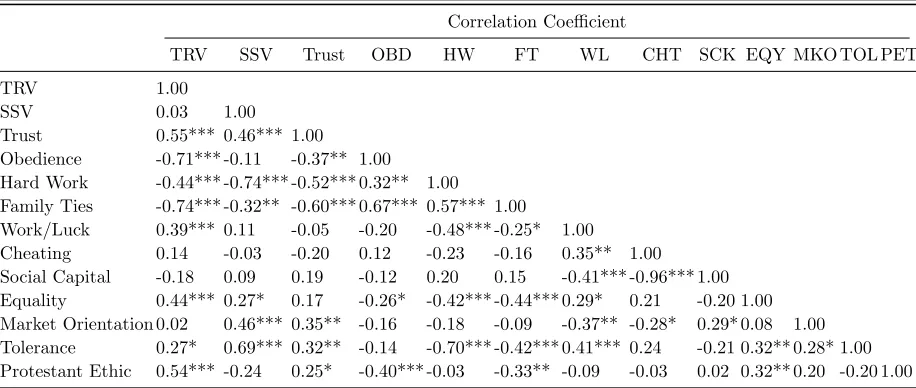
Additionally, the research analyzes other country-level cultural measures, which have been previously been used in the literature or which should capture elements highlighted by it. In particular, it focuses on the following additional 12 measures: Generalized Trust (Trust), Obedience (OBD), Hard Work (HW), Family Ties (FT), Work vs. Luck (WL), Cheating (CHT), Social Capital (SCK), Caring about Equality (EQY), Market Orientation (MKO), Tolerance (TOL), and Protestant Ethic (PET). Table 2 shows the pairwise correla-tions between the WVS measures across countries. As expected, Survival-Self-Expression and Traditional-Rational Values are highly correlated with the other cultural measures. More-over, and in contrast to the Hofstede measures, many WVS based measures are highly correlated with each other, suggesting they capture similar elements. In particular, cultural traits like Family Ties, Obedience and Trust correlate strongly with each other.2
For each Hofstede and WVS cultural dimension two distance measures are constructed for each country pair. In particular, given a cultural trait X, the absolute pairwise distance
between countriesiandj,Xij, is given byXij =|Xi−Xj|, and therelative pairwise distance
between countries i and j, XR
ij, is given by XijR =|XiU S−XjU S|, where it is assumed that
the technological frontier is the US, andXiU S is the absolute distance between countryiand
the US. Interestingly, while the correlation between the different measures of culture can be low, as shown in Table 1, the absolute cultural differences are generally highly correlated as shown in Tables A.1-A.2.
Finally, in order to capture a general level of cultural difference, an additional measure is constructed based on the Survival-Self-Expression and Traditional-Rational Values. This
2
Table 2: Correlation between WVS Cultural Measures (Levels)
Correlation Coefficient
TRV SSV Trust OBD HW FT WL CHT SCK EQY MKO TOL PET
TRV 1.00
SSV 0.03 1.00
Trust 0.55*** 0.46*** 1.00
Obedience -0.71*** -0.11 -0.37** 1.00
Hard Work -0.44*** -0.74*** -0.52*** 0.32** 1.00
Family Ties -0.74*** -0.32** -0.60*** 0.67*** 0.57*** 1.00
Work/Luck 0.39*** 0.11 -0.05 -0.20 -0.48*** -0.25* 1.00
Cheating 0.14 -0.03 -0.20 0.12 -0.23 -0.16 0.35** 1.00
Social Capital -0.18 0.09 0.19 -0.12 0.20 0.15 -0.41*** -0.96*** 1.00
Equality 0.44*** 0.27* 0.17 -0.26* -0.42*** -0.44*** 0.29* 0.21 -0.20 1.00
Market Orientation 0.02 0.46*** 0.35** -0.16 -0.18 -0.09 -0.37** -0.28* 0.29* 0.08 1.00
Tolerance 0.27* 0.69*** 0.32** -0.14 -0.70*** -0.42*** 0.41*** 0.24 -0.21 0.32** 0.28* 1.00
Protestant Ethic 0.54*** -0.24 0.25* -0.40*** -0.03 -0.33** -0.09 -0.03 0.02 0.32** 0.20 -0.20 1.00
Notes: *** denotes statistical significance at the 1% level, ** at the 5% level, and * at the 10% level, all for two-sided hypothesis tests.
WVS cultural distance is defined as the Manhattan distance between countries on the plane
determined by these two measures. Based on this measure, the largest cultural distance in the sample is between Sweden and Tanzania and the smallest is between Mexico and the Dominican Republic. Therelative WVS cultural distance is constructed in the same manner as other relative distances.
3.2
Genetic Distances
The analysis employs genetic distances as a measure of the time since two populations diverged from a common ancestor. The genetic distance data employed in the analysis is taken from Spolaore and Wacziarg (2009a), who constructed genetic distances between countries based on ethnic-level data from Cavalli-Sforza et al. (1994). Spolaore and Wacziarg (2009a) provide 3 measures of genetic distance for each country pair: (i) FST-dominant,
which is the distance between the major ethnic groups of each country in a pair; (ii) FST
-weighted, which is the ethnic-level weighted genetic distance between two randomly selected
individuals (one from each country); and (iii) FST-1500, which proxies the genetic distance
between countries as of 1500. The analysis employsFST-weightedas the main genetic distance
measure, since it better represents the average genetic distance between countries and is the measure used in the main analysis of Spolaore and Wacziarg (2009a,b, 2012, 2013a,b).3
Based on these genetic distances, the analysis constructs relative genetic distances for each country pair in a similar fashion as other relative distances.
3
3.3
Additional Controls
Cultural differences between societies are not only affected by the time since they shared a common ancestor, but also by other elements that affect ancestry, like religion and language, and by differences in other determinants of culture like geography (Alesina et al., 2013; Galor and ¨Ozak, 2014). Thus, in order to overcome potential biases due to omitted factors, this research accounts for a large set of additional pairwise differences. In particular, the analysis accounts for geographic, linguistic and religious distances, differences in a large set of geographical conditions (absolute latitude, elevation, agricultural and caloric suitability, being landlocked or islands, climatic conditions, etc.), and a full set of pairwise continental fixed effects (whether one or both or none of the countries in the pair are in a specific continent). Importantly, the analysis accounts for country fixed effects, which ensures that only non-linear pairwise omitted factors could potentially bias the results.
4
Empirical Analysis
This section explores empirically the relation between absolute and relative cultural distances and economic development. Additionally, it examines the relation between differences in cultural traits and various proxies of cultural differences used in the literature. In particular, it analyzes the relation between the Hofstede and WVS cultural distances introduced in the previous section and genetic, linguistic, and religious distances.
4.1
Cultural Differences and Genetic Distances
This section analyzes the association between cultural differences and genetic, linguistic, and religious distances across countries. Genetic distances have played an essential role in the literature as a proxy of cultural differences. Thus, it is only natural that it also plays a central role in the following analysis. In particular, while the interpretation of genetic distances as a measure of the time since two populations shared a common ancestor is well established, which cultural differences are captured by genetic distances is poorly understood. For example, using genetic distances among European regions, Desmet et al. (2011) find suggestive evidence that genetic distances capture generic cultural differences among these regions. On the other hand, Giuliano et al. (2006) suggest that genetic distances among European regions capture transportation costs and not cultural differences.4
4
This research differs from the previous literature in various aspects: (i) it explores the relation between genetic distances and actual measures of differences in cultural values that ought to be relevant to economic development at the country level. This allows the identifi-cation of the potential cultural channels that genetic distance is proxying. (ii) It accounts for the effect of other geographical distances and country fixed effects. Thus, accounting for the potential effect of transportation costs and other geographically determined effects. (iii) It accounts for linguistic and religious distances, which also capture common ancestry, in order to identify the main channels though which ancestry can play a role in cultural differences. (iv) It includes a large sample of countries and is not limited to a specific region or continent.
The general empirical specification used in this section is
Cultural distanceij =α+βGGDij +βLLDij+βRRDij +
X
k
γkXijk +ci+cj+ǫij,
whereGDij is the genetic distance between countriesiandj,LDij is their linguistic distance,
RDij is their religious distance,
Xk
ij kis a large set of additional pairwise controls, including
geographic distances and differences in geographic factors (absolute latitude, landlocked, island, close to cost or river, terrain ruggedness, agricultural and caloric suitability, climatic zones, etc.), common history (ever same country, ever in colonial relationship, have common colonizer), difference in the number of years since the Neolithic transition, a complete set of continental fixed effects (whether one, both or none of the countries in the pair belong to a specific continent),ci andcj are country fixed effects, andǫij is an error term. Given that the
construction of cultural differences can potentially generate correlation across observations for each country i, the analysis clusters standard errors at two levels, one for each country in the pair (Cameron et al., 2011).
4.1.1 Hofstede Cultural Dimensions
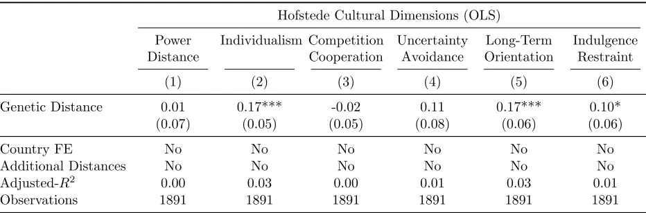
This section uses differences in Hoftsede’s cultural dimensions as the dependent variables in the analysis. Table 3 shows the results of the Ordinary Least Squares (OLS) regres-sion between differences in Hofstede’s cultural dimenregres-sions and genetic distances without any additional controls. As can be seen there, differences in Individualism, Long-Term Orien-tation, and Indulgence vs. Restraint are significantly correlated with genetic distances. In particular, the estimated coefficients imply that a one-standard deviation increase in genetic distance between countriesiandjis associated with about a half standard deviation increase in their difference in Individualism.5
5
Table 3: Hofstede’s Cultural Dimensions and Genetic Distances (Unconditional)
Hofstede Cultural Dimensions (OLS) Power
Distance
Individualism Competition Cooperation
Uncertainty Avoidance
Long-Term Orientation
Indulgence Restraint
(1) (2) (3) (4) (5) (6)
Genetic Distance 0.01 0.17*** -0.02 0.11 0.17*** 0.10*
(0.07) (0.05) (0.05) (0.08) (0.06) (0.06)
Country FE No No No No No No
Additional Distances No No No No No No
Adjusted-R2
0.00 0.03 0.00 0.01 0.03 0.01
Observations 1891 1891 1891 1891 1891 1891
[image:18.612.73.544.324.476.2]Notes: This table shows the simple correlation between each of Hofstede’s cultural dimensions and genetic distance. Coefficients are standardized betas. Two-way clustered standard errors in parentheses. *** denotes statistical significance at the 1% level, ** at the 5% level, and * at the 10% level, all for two-sided hypothesis tests.
Table 4: Hofstede’s Cultural Dimensions and Genetic Distances (Fixed Effects)
Hofstede Cultural Dimensions (OLS) Power
Distance
Individualism Competition Cooperation
Uncertainty Avoidance
Long-Term Orientation
Indulgence Restraint
(1) (2) (3) (4) (5) (6)
Genetic Distance 0.18** 0.48*** 0.01 0.16** 0.07 0.11**
(0.08) (0.09) (0.02) (0.08) (0.05) (0.06)
Country FE Yes Yes Yes Yes Yes Yes
Additional Distances No No No No No No
Adjusted-R2
0.42 0.27 0.55 0.33 0.30 0.37
Observations 1891 1891 1891 1891 1891 1891
Notes: This table shows the correlation between each of Hofstede’s cultural dimensions and genetic distance after accounting for country fixed effect. Coefficients are standardized betas. Two-way clustered standard errors in parentheses. *** denotes statistical significance at the 1% level, ** at the 5% level, and * at the 10% level, all for two-sided hypothesis tests.
Table 4 accounts for country fixed effects in order to capture any unobserved time-invariant country specific characteristics. The results show that once country specific unob-servables are accounted for, the coefficients generally increase both in terms of magnitude and significance, particularly for Power distance. Still, genetic distances might be capturing the confounding effect of other differences among countries.
The potential confounding effect of other differences among countries is explored in Table 5. This table establishes that once one accounts for country fixed effects, pairwise differ-ences in geographical characteristics and continental fixed effects, Individualism is the only cultural distance that remains economically and statistically significantly correlated with
Table 5: Hofstede’s Cultural Dimensions and Genetic Distances (Geography + FE)
Hofstede Cultural Dimensions (OLS) Power
Distance
Individualism Competition Cooperation
Uncertainty Avoidance
Long-Term Orientation
Indulgence Restraint
(1) (2) (3) (4) (5) (6)
Genetic Distance 0.14 0.32** -0.01 0.08 -0.09 -0.01
(0.10) (0.14) (0.04) (0.07) (0.13) (0.10)
Country FE Yes Yes Yes Yes Yes Yes
Additional Distances Yes Yes Yes Yes Yes Yes
Adjusted-R2
0.45 0.42 0.55 0.38 0.38 0.43
Observations 1830 1830 1830 1830 1830 1830
Notes: This table shows the correlation between each of Hofstede’s cultural dimensions and genetic distance after accounting for country fixed effects, pairwise geographical differences, and continental fixed effects. Coefficients are standardized betas. Two-way clustered standard errors in parentheses. *** denotes statistical significance at the 1% level, ** at the 5% level, and * at the 10% level, all for two-sided hypothesis tests.
genetic distance. This suggests that among the cultural values identified by Hofstede et al. (2010), Individualism is potentially the main cultural value that genetic distance is proxying for. Moreover, these results suggest that Individualism is the only trait for which common ancestry, as measured by genetic distance, plays a role.
In order to further analyze the role of common ancestry, Table 6 additionally accounts for linguistic and religious distances, which also capture common ancestry and historical expe-rience. Interestingly, except for the Competition-Cooperation value, all cultural differences are positively correlated with either linguistic or genetic distances. In particular, Power Distance, Individualism, Uncertainty Avoidance, Long-Term Orientation, and Indulgence vs Restraint are statistically and economically significantly correlated with linguistic distances. On the other hand, only Individualism remains statistically significantly correlated with ge-netic distances. Furthermore, religious distance is not statistically significantly correlated with any of the differences in cultural dimensions across countries. These results support the view that common ancestry plays a central role in the generation of cultural differences. Moreover, they suggest that linguistic distances capture a wider set of cultural differences than genetic distances, which seem to only correlate with differences in Individualism.
Table 6: Hofstede’s Cultural Dimensions and Genetic Distances (Linguistic and Religious Distances)
Hofstede Cultural Dimensions (OLS) Power
Distance
Individualism Competition Cooperation
Uncertainty Avoidance
Long-Term Orientation
Indulgence Restraint
(1) (2) (3) (4) (5) (6)
Genetic Distance 0.13 0.31** -0.03 0.06 -0.09 -0.03
(0.09) (0.13) (0.05) (0.08) (0.11) (0.08)
Linguistic Distance 0.31*** 0.35** 0.04 0.33*** 0.16*** 0.23***
(0.11) (0.18) (0.07) (0.09) (0.06) (0.09)
Religious Distance 0.10* 0.05 0.07 0.06 0.04 0.06
(0.06) (0.04) (0.06) (0.09) (0.09) (0.07)
Country FE Yes Yes Yes Yes Yes Yes
Additional Distances Yes Yes Yes Yes Yes Yes
Adjusted-R2
0.47 0.44 0.54 0.40 0.38 0.45
Observations 1711 1711 1711 1711 1711 1711
Notes: This table shows the correlation between each of Hofstede’s cultural dimensions and genetic distance after accounting for country fixed effects, pairwise geographical differences, continental fixed effects, and linguistic and religious distances. Coefficients are standardized betas. Two-way clustered standard errors in parentheses. *** denotes statistical significance at the 1% level, ** at the 5% level, and * at the 10% level, all for two-sided hypothesis tests.
results do not change, they weaken the statistical significance of the positive association between genetic distance and Individualism, and increase the significance of the negative association between genetic distance and differences between Indulgence vs. Restraint.
Overall, the analysis of this subsection suggests that genetic distances capture mostly the effects of Individualism, while linguistic distances capture the effects of differences in a larger set of cultural values. These results might explain the economic and statistical significance of both Individualism and genetic distances found in the literature (Gorodnichenko and Roland, 2011; Spolaore and Wacziarg, 2009a). Additionally, it supports the view that common ancestry explains commonality in cultural values and the persistence of culture (Alesina and Giuliano, 2013; Galor and ¨Ozak, 2014; Galor et al., 2016; Guiso et al., 2006).
4.1.2 WVS Cultural Measures
Table 7: Hofstede’s Cultural Dimensions and Genetic Distances (IV)
Hofstede Cultural Dimensions (IV) Power
Distance
Individualism Competition Cooperation
Uncertainty Avoidance
Long-Term Orientation
Indulgence Restraint
(1) (2) (3) (4) (5) (6)
Genetic Distance 0.04 0.29* -0.10 0.13 -0.22 -0.26**
(0.11) (0.16) (0.09) (0.10) (0.14) (0.11)
Linguistic Distance 0.30*** 0.35** 0.04 0.34*** 0.16*** 0.22**
(0.10) (0.16) (0.06) (0.09) (0.05) (0.09)
Religious Distance 0.11** 0.05 0.07 0.05 0.06 0.09
(0.05) (0.04) (0.06) (0.08) (0.08) (0.07)
Country FE Yes Yes Yes Yes Yes Yes
Additional Distances Yes Yes Yes Yes Yes Yes
Adjusted-R2
0.44 0.41 0.52 0.37 0.35 0.41
Observations 1711 1711 1711 1711 1711 1711
F-statistic (first stage) 15.82 15.82 15.82 15.82 15.82 15.82
Notes: This table shows the causal relationship between each of Hofstede’s cultural dimensions and genetic distance after accounting for country fixed effects, pairwise geographical differences, continental fixed effects, and linguistic and religious distances. Genetic distance in 1500CE is used as an instrument for contemporary genetic distance. Coefficients are stan-dardized betas. Two-way clustered standard errors in parentheses. *** denotes statistical significance at the 1% level, ** at the 5% level, and * at the 10% level, all for two-sided hypothesis tests.
the expected effect that genetic distance ought to have on cultural distances due to common ancestry.
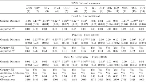
The negative correlation between genetic distance and Survival-Self-Expression and Mar-ket Orientation might be generated due to omitted variable bias. In particular, as estab-lished in Table 8-Panel B, once one accounts for country fixed effects, the coefficient on genetic distance becomes non-negative for all WVS cultural values including the Survival-Self-Expression and Market Orientation. Moreover, the coefficient increases in economic and statistical significance for the Tradition-Rational, Generalized Trust, Obedience, Hard Work and Family Ties.
Table 8-Panel C establishes that genetic distances are not statistically and economically significantly correlated with Tradition-Rational and Survival-Self-Expression once one ad-ditionally accounts for other geographical and historical differences. On the other hand, Generalized Trust, Obedience, Hard Work and Family Ties remain statistically and econom-ically significantly correlated with genetic distances. This suggests that genetic distances capture mainly differences in cultural traits that are expected to have economic effects.
Table 8: WVS Cultural Measures and Genetic Distances
WVS Cultural measures
WVS TRV SSV Trust OBD HW FT WL CHT SCK EQY MKO TOL PET
(1) (2) (3) (4) (5) (6) (7) (8) (9) (10) (11) (12) (13) (14)
Panel A: Unconditional
Genetic Distance -0.06 0.17*** -0.19*** 0.12** 0.36*** 0.22** 0.13* -0.00 0.03 0.03 0.05 -0.14** -0.09** 0.07
(0.05) (0.06) (0.04) (0.06) (0.07) (0.09) (0.07) (0.06) (0.05) (0.05) (0.06) (0.06) (0.04) (0.05)
Adjusted-R2
0.00 0.02 0.03 0.01 0.10 0.05 0.01 0.00 0.00 0.00 0.00 0.02 0.01 0.00
Panel B: Fixed Effects
Genetic Distance 0.09 0.33*** 0.12** 0.20*** 0.38*** 0.35*** 0.27*** 0.08 -0.00 0.00 0.10 0.00 0.09* 0.12*
(0.06) (0.08) (0.05) (0.04) (0.10) (0.10) (0.08) (0.06) (0.01) (0.01) (0.07) (0.03) (0.05) (0.07)
Country FE Yes Yes Yes Yes Yes Yes Yes Yes Yes Yes Yes Yes Yes Yes
Adjusted-R2
0.61 0.26 0.53 0.53 0.41 0.34 0.46 0.48 0.44 0.45 0.32 0.52 0.42 0.30
Panel C: Geography + Fixed Effects
Genetic Distance 0.04 0.08 0.05 0.13** 0.23** 0.34*** 0.16*** 0.03 -0.03* -0.03 0.06 -0.00 -0.01 0.04
(0.05) (0.07) (0.05) (0.05) (0.10) (0.09) (0.06) (0.06) (0.02) (0.03) (0.06) (0.03) (0.05) (0.07)
Country FE Yes Yes Yes Yes Yes Yes Yes Yes Yes Yes Yes Yes Yes Yes
Additional Distances Yes Yes Yes Yes Yes Yes Yes Yes Yes Yes Yes Yes Yes Yes
Adjusted-R2
0.62 0.57 0.54 0.56 0.53 0.39 0.58 0.49 0.44 0.45 0.36 0.52 0.46 0.35
Observations 3486 3486 3486 4005 1891 1485 2080 3570 3655 3655 2850 2701 3828 4005
Notes: This table shows correlation between each of the WVS cultural measures and genetic distance. Panel A shows the correlation without any controls. Panel B accounts for country fixed effects. Panel C additionally accounts for pairwise geographical differences and continental fixed effects. Each column shows the relation to with respect to one measure, where the WVS measures are WVS distance, Survival vs. Self-Expression Values (SSV), Traditional vs. Secular-Rational Values (TRV), Generalized Trust (Trust), Obedience (OBD), Hard Work (HW), Family Ties (FT), Work vs. Luck (WL), Cheating (CHT), Social Capital (SCK), Caring about Equality (EQY), Market Orientation (MKO), Tolerance (TOL), and Protestant Ethic (PET), see section 3 for additional information on measures. Coefficients are standardized betas. Two-way clustered standard errors in parentheses. *** denotes statistical significance at the 1% level, ** at the 5% level, and * at the 10% level, all for two-sided hypothesis tests.
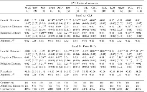
Survival-Self-Expression, Tolerance and Protestant Ethic. On the other hand, and also in contrast to the analysis based on the Hofstede measures, religious distances are statistically and economically significantly correlated with various measures, including the Survival-Self-Expression, Hard Work, and Tolerance.
Table 9: WVS Cultural Measures and Ancestry
WVS Cultural measures
WVS TRV SSV Trust OBD HW FT WL CHT SCK EQY MKO TOL PET
(1) (2) (3) (4) (5) (6) (7) (8) (9) (10) (11) (12) (13) (14)
Panel A: OLS
Genetic Distance 0.03 0.07 0.03 0.13** 0.23** 0.31** 0.15*** 0.02 -0.03* -0.03 0.05 -0.01 -0.03 0.03
(0.05) (0.07) (0.04) (0.05) (0.09) (0.12) (0.06) (0.05) (0.02) (0.02) (0.06) (0.03) (0.06) (0.07)
Linguistic Distance 0.07 0.03 0.21** -0.02 0.09 0.05 0.02 -0.01 0.00 0.00 0.06 0.15 0.17** 0.19**
(0.07) (0.04) (0.10) (0.05) (0.05) (0.11) (0.05) (0.04) (0.04) (0.04) (0.05) (0.09) (0.08) (0.09)
Religious Distance 0.02 0.04* 0.20*** 0.03 -0.03 0.24*** 0.08* 0.07 0.04 0.03 0.04 -0.01 0.14*** -0.02
(0.03) (0.03) (0.04) (0.02) (0.03) (0.08) (0.05) (0.05) (0.03) (0.03) (0.04) (0.02) (0.05) (0.04)
Adjusted-R2
0.62 0.58 0.58 0.55 0.53 0.42 0.58 0.50 0.44 0.45 0.36 0.52 0.47 0.36
Panel B: Panel B: IV
Genetic Distance -0.01 0.03 -0.02 0.10** 0.11 0.34*** 0.12* -0.02 -0.06*** -0.06*** 0.02 -0.06** -0.16*** -0.15**
(0.03) (0.05) (0.04) (0.04) (0.08) (0.08) (0.06) (0.04) (0.01) (0.01) (0.05) (0.03) (0.05) (0.06)
Linguistic Distance 0.08 0.04 0.25** -0.02 0.07* 0.04 0.03 -0.01 0.00 0.01 0.06 0.16* 0.21** 0.23**
(0.07) (0.05) (0.11) (0.05) (0.04) (0.10) (0.05) (0.05) (0.04) (0.04) (0.04) (0.09) (0.10) (0.10)
Religious Distance 0.02 0.05* 0.21*** 0.03 -0.03 0.25*** 0.09** 0.08 0.04 0.03 0.04 -0.01 0.15*** -0.02
(0.03) (0.02) (0.04) (0.02) (0.03) (0.07) (0.04) (0.05) (0.03) (0.03) (0.04) (0.02) (0.05) (0.04)
F-statistic 91.34 91.34 91.34 88.29 36.32 141.59 33.47 56.52 90.66 90.66 90.48 86.86 90.15 88.29
Adjusted-R2
0.61 0.56 0.56 0.54 0.51 0.39 0.56 0.49 0.43 0.43 0.34 0.51 0.45 0.33
Country FE Yes Yes Yes Yes Yes Yes Yes Yes Yes Yes Yes Yes Yes Yes
Additional Distances Yes Yes Yes Yes Yes Yes Yes Yes Yes Yes Yes Yes Yes Yes
Observations 3486 3486 3486 3916 1891 1485 2080 3486 3655 3655 2850 2701 3741 3916
Notes: Panel A of the table shows the coefficients of an Ordinary Least Squares (OLS) regression between each of the WVS cultural measures and genetic distance after accounting for country fixed effects, pairwise geographical differences, continental fixed effects, and linguistic and religious distances. Panel B uses an instrumental variable (IV) approach to show the casual effect of the genetic distance on each of WVS cultural measures after accounting for all controls. Each column shows the relation to with respect to one measure, where the WVS measures are WVS distance, Survival vs. Self-Expression Values (SSV), Traditional vs. Secular-Rational Values (TRV), Generalized Trust (Trust), Obedience (OBD), Hard Work (HW), Family Ties (FT), Work vs. Luck (WL), Cheating (CHT), Social Capital (SCK), Caring about Equality (EQY), Market Orientation (MKO), Tolerance (TOL), and Protestant Ethic (PET), see section 3 for additional information on measures. Coefficients are standardized betas. Two-way clustered standard errors in parentheses. *** denotes statistical significance at the 1% level, ** at the 5% level, and * at the 10% level, all for two-sided hypothesis tests.
element behind comparative development. Finally, given the high correlation between Indi-vidualism and Generalized Trust, it is reassuring to find similar results using both measures, even though the results are based on different samples.
4.2
Income and Cultural Differences
The analysis generalizes the empirical specification in Spolaore and Wacziarg (2009a) in order to include absolute and relative cultural differences. Thus, the empirical specification used in the analysis is
yij =α+βGRGD R
ij +βCCij +βCRCij +βLLDij+βLRLD R
ij +βRRDij +βRRRD R ij
+X
k
γkXijk +ci +cj+ǫij,
where the dependent variable, yij, is the absolute value of the pairwise difference in log
income per capita in 1995 between country i and j, GDR
ij is the relative genetic distance
to the US between countries i and j, CDij is their cultural distance, CDijR is their relative
cultural distance, LDij is their linguistic distance, LDRij is their relative linguistic distance,
RDij is their religious distance,RDijRis their relative religious distance,
Xk
ij k is a large set
of additional pairwise controls, including geographic distances and differences in geographic factors (absolute latitude, landlocked, island, close to cost or river, terrain ruggedness, agri-cultural and caloric suitability, climatic zones, etc.), common history (ever same country, ever in colonial relationship, have common colonizer), difference in the number of years since the Neolithic transition, a complete set of continental fixed effects (whether one, both or none of the countries in the pair belong to a specific continent), ci and cj are country fixed
effects, and ǫij is an error term.6 Given that the construction of differences can potentially
generate correlation across observations for each country i, the analysis clusters standard errors at two levels, one for each country in the pair (Cameron et al., 2011).
4.2.1 Hofstede Cultural Dimensions
This section explores the direct and barrier effects of the Hofstede cultural dimensions. Table 10 explores the correlation between differences in economic development, relative genetic distances and cultural distances. Column 1 shows that genetic distance relative to frontier is significantly associated with income differences for the subset of countries for which the cultural Hofstede dimensions is available.7
Columns 2-7 account for the absolute cultural distances in Individualism, Power
Dis-6
In order to facilitate comparison with Spolaore and Wacziarg (2009a), the results shown in the main body of the paper use only the subset of controls used by them. The appendix includes the full set of controls, which were employed in section 4.1.
7
tance, Competition vs Cooperation, Uncertainty Avoidance, Long-Term Orientation, and Indulgence vs Restraint, while columns 9-14 account for the relative distances for these same cultural values. The results show that absolute and relative distances in Individualism and Power Distance are positively economically and statistically associated with differences in economic development. Additionally, relative distances in Indulgence vs Restraint are also strongly associated with economic development. Columns 8 and 15 respectively account for all absolute and relative cultural distances jointly with similar results.
The results of columns 2 and 9 establish that once one accounts for differences in Indi-vidualism, the genetic distance relative to the US ceases to be associated with differences in economic development. This suggests that genetic distances relative to the US might be capturing the effect of differences in Individualism. This view is supported by the re-sults of section 4.1.1, which established the strong association between genetic distances and differences in Individualism. Furthermore, as shown in Table B.3, relative distances in Individualism are the only relative cultural trait that is economically and statistically significantly correlated with relative genetic distances.
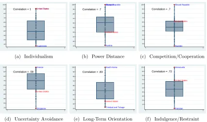
While these results suggest that relative genetic distances might be capturing the barrier effect of Individualism, this interpretation is subject to the problem of observational equiv-alence. In particular, given that the US has the highest value of Individualism (see Figure 2), the absolute and relative distances are observationally equivalent. So, although column 9 would suggest a barrier effect of individualism, this might just be capturing the direct effect that has been obscured by the observational equivalence. Moreover, in light of this observational equivalence, the results of section 4.1.1 and Tables B.4-B.6, it is possible that relative genetic distances do not capture the barrier effect, but instead the direct effects of culture.
Although these results suggest one potential mechanism being captured by relative ge-netic distances, it does not help in the identification of the direct vs barrier effects of these various cultural values. In order to analyze this further, Table 11 accounts jointly for both absolute and relative cultural distances. The results show that only absolute distances in Individualism and Power Distance, and relative distances in Indulgence vs Restraint are positively economically and statistically significantly associated with differences in economic development. A horse race between the absolute and relative distances of all the Hofstede cultural values finds that only Individualism and Indulgence vs Restraint remain positively strongly associated with economic development.
Table 10: Hofstede Cultural Dimensions
Differences in log per capita income (1995)
Direct Effect of Culture Barrier Effect of Culture
(1) (2) (3) (4) (5) (6) (7) (8) (9) (10) (11) (12) (13) (14) (15) Genetic Distance 0.15** 0.10 0.14** 0.15** 0.14** 0.15** 0.15** 0.11** 0.10 0.14** 0.15** 0.15** 0.15** 0.15** 0.11* relative to US (0.07) (0.06) (0.06) (0.07) (0.07) (0.07) (0.07) (0.06) (0.06) (0.07) (0.07) (0.07) (0.07) (0.07) (0.06) Individualism 0.21*** 0.15**
(0.07) (0.07)
Power Distance 0.20*** 0.15**
(0.06) (0.06)
Compet/Cooper -0.07** -0.11*** (0.03) (0.03)
Uncertainty Avoid 0.06 0.04
(0.05) (0.05) Long-Term Orient -0.06 -0.06
(0.04) (0.05) Indulgence/Restraint 0.11 0.10
(0.07) (0.06)
Individualism, 0.21*** 0.16**
relative to US (0.07) (0.07)
Power Distance, 0.15** 0.09
relative to US (0.07) (0.07)
Compet/Cooper, -0.03 -0.06**
relative to US (0.03) (0.03)
Uncertainty Avoid, -0.00 -0.02
relative to US (0.03) (0.03)
Long-Term Orient, -0.06* -0.07*
relative to US (0.03) (0.04)
Indulg/Restraint, 0.22*** 0.20***
relative to US (0.07) (0.06)
Adjusted-R2
0.02 0.06 0.06 0.03 0.03 0.03 0.03 0.11 0.06 0.04 0.02 0.02 0.03 0.07 0.12 Observations 1830 1830 1830 1830 1830 1830 1830 1830 1830 1830 1830 1830 1830 1830 1830
Notes: This table shows correlation between absolute log-differences in income per capita in 1995 and absolute and relative cultural distances based on Hofstede et al. (2010) cultural values. Coefficients are standardized betas. Two-way clustered standard errors in parentheses. *** denotes statistical significance at the 1% level, ** at the 5% level, and * at the 10% level, all for two-sided hypothesis tests.
United States
Guatemala
United States
Correlation = 1
10 20 30 40 50 60 70 80 90 100 .5 1.5 (a) Individualism Malaysia Slovak Republic Austria United States
Correlation = .7
10 20 30 40 50 60 70 80 90 100 .5 1.5
(b) Power Distance
Slovak Republic
Sweden
United States
Correlation = .7
10 20 30 40 50 60 70 80 90 100 .5 1.5 (c) Competition/Cooperation Greece Singapore United States
Correlation = .58
10 20 30 40 50 60 70 80 90 100 .5 1.5
(d) Uncertainty Avoidance
South Korea
Trinidad and Tobago
United States
Correlation = .83
10 20 30 40 50 60 70 80 90 100 .5 1.5
(e) Long-Term Orientation
Venezuela
Pakistan
United States
Correlation = .72
[image:27.612.94.520.73.324.2]10 20 30 40 50 60 70 80 90 100 .5 1.5 (f) Indulgence/Restraint
Figure 2: Location of U.S. in the Distribution of Hofstede Dimensions
economic development. Furthermore, neither relative genetic distances nor any of the other distances is statistically significantly associated with economic development. The results of Table 12 also show that in a horse race with all absolute and relative distances, only the absolute distance in Power Distance remains statistically and economically associated with economic development.
Given the potential bias due to omitted variables, Table 13 additionally accounts for geo-graphical differences, pairwise continental fixed effects, other measures of common ancestry, as well as relative linguistic and religious distances. The results are qualitatively and quanti-tatively similar to the previous ones. In particular, absolute distances in Individualism and Power Distance, and relative distance in Indulgence vs Restraint are positive economically statistically significantly associated with differences in economic development. In particular, the estimates suggest that a one standard deviation increase in the absolute distance in In-dividualism is associated with a 0.24 standard deviation increase in log-absolute differences in income per capita. Similarly, a one standard deviation increase in the absolute distance in Power Distance is associated with a 0.41 standard deviation increase in log-absolute dif-ferences in income per capita. On the other hand, a one standard deviation increase in the relative distance in Indulgence vs Restraint is associated with a 0.28 standard deviation increase in log-absolute differences in income per capita.
Table 11: Hofstede Cultural Dimensions and Income (Unconditional)
Differences in log per capita income (1995)
(1) (2) (3) (4) (5) (6) (7) (8)
Genetic Distance relative to US 0.15** 0.10 0.14** 0.15** 0.14** 0.15** 0.15** 0.10* (0.07) (0.06) (0.07) (0.07) (0.07) (0.07) (0.07) (0.05)
Individualism 0.21*** 0.14**
(0.07) (0.07)
Power Distance 0.20*** 0.11*
(0.05) (0.06)
Compet/Cooper -0.11*** -0.11**
(0.04) (0.04)
Uncertainty Avoid 0.10 0.10
(0.07) (0.07)
Long-Term Orient 0.00 0.09
(0.14) (0.15)
Indulgence/Restraint -0.09*** -0.09***
(0.02) (0.03)
Individualism relative to US 0.00 0.00
(0.00) (0.00)
Power Distance relative to US 0.00 0.03
(0.08) (0.08)
Compet/Cooper relative to US 0.05 0.01
(0.04) (0.04)
Uncertainty Avoid relative to US -0.07 -0.09
(0.05) (0.06)
Long-Term Orient relative to US -0.07 -0.14
(0.13) (0.14)
Indulg/Restraint relative to US 0.28*** 0.25***
(0.07) (0.07)
Adjusted-R2 0.02 0.06 0.06 0.03 0.03 0.03 0.08 0.14
Observations 1830 1830 1830 1830 1830 1830 1830 1830
Notes: This table explores the direct and barrier effects of Hofstede’s cultural values by running a horse race between absolute and relative cultural distances. Coefficients are standardized betas of an Ordinary Least Squares (OLS) regression without additional controls. Two-way clustered standard errors in parentheses. *** denotes statistical significance at the 1% level, ** at the 5% level, and * at the 10% level, all for two-sided hypothesis tests.
Table 12: Hofstede Cultural Dimensions and Income (Fixed Effects)
Differences in log per capita income (1995)
(1) (2) (3) (4) (5) (6) (7) (8)
Genetic Distance relative to US 0.14* 0.06 0.11* 0.14* 0.14* 0.14* 0.12* 0.06 (0.08) (0.10) (0.07) (0.08) (0.07) (0.08) (0.07) (0.06)
Individualism 0.25*** 0.15
(0.09) (0.09)
Power Distance 0.43*** 0.27***
(0.08) (0.09)
Compet/Cooper 0.03 0.01
(0.05) (0.05)
Uncertainty Avoid 0.06 0.07*
(0.06) (0.04)
Long-Term Orient 0.13 0.13
(0.11) (0.11)
Indulgence/Restraint -0.07 -0.03
(0.06) (0.06)
Individualism relative to US 0.00 0.00
(0.00) (0.00)
Power Distance relative to US -0.12 -0.08
(0.09) (0.08)
Compet/Cooper relative to US -0.00 -0.01
(0.04) (0.04)
Uncertainty Avoid relative to US -0.02 -0.07 (0.04) (0.06) Long-Term Orient relative to US -0.12 -0.13
(0.11) (0.11) Indulg/Restraint relative to US 0.26*** 0.17*
(0.10) (0.09)
Country FE Yes Yes Yes Yes Yes Yes Yes Yes
Adjusted-R2
0.44 0.49 0.51 0.44 0.44 0.44 0.47 0.53 Observations 1830 1830 1830 1830 1830 1830 1830 1830
Notes: This table explores the direct and barrier effects of Hofstede’s cultural values by running a horse race between absolute and relative cultural distances. Coefficients are standardized betas of an Ordinary Least Squares (OLS) regression after accounting for country fixed effects. Two-way clustered standard errors in parentheses. *** denotes statistical significance at the 1% level, ** at the 5% level, and * at the 10% level, all for two-sided hypothesis tests.
Table 13: Hofstede Cultural Dimensions and Income (All Controls)
Differences in log per capita income (1995)
(1) (2) (3) (4) (5) (6) (7) (8)
Genetic Distance relative to US 0.11 0.06 0.10 0.11 0.11 0.11 0.11 0.07 (0.10) (0.08) (0.07) (0.09) (0.07) (0.08) (0.07) (0.06)
Individualism 0.24*** 0.15*
(0.08) (0.09)
Power Distance 0.41*** 0.26***
(0.09) (0.09)
Compet/Cooper 0.00 -0.01
(0.05) (0.05)
Uncertainty Avoid 0.07 0.05
(0.06) (0.04)
Long-Term Orient 0.10 0.11
(0.10) (0.09)
Indulgence/Restraint -0.09 -0.04
(0.07) (0.06)
Individualism relative to US 0.00 0.00
(0.00) (0.00)
Power Distance relative to US -0.12 -0.07
(0.10) (0.09)
Compet/Cooper relative to US -0.00 0.01
(0.05) (0.04)
Uncertainty Avoid relative to US -0.03 -0.07
(0.05) (0.06)
Long-Term Orient relative to US -0.13 -0.12
(0.10) (0.10)
Indulg/Restraint relative to US 0.28** 0.20*
(0.11) (0.10) Linguistic Distance 0.12* 0.09 0.05 0.12* 0.12* 0.12* 0.13* 0.06
(0.07) (0.06) (0.06) (0.07) (0.07) (0.06) (0.07) (0.07) Religious Distance -0.10 -0.07 -0.12 -0.10 -0.11 -0.09 -0.08 -0.08
(0.13) (0.13) (0.12) (0.13) (0.13) (0.13) (0.13) (0.13) Linguistic Distance relative to the US 0.13* 0.07 0.07 0.13* 0.14* 0.14* 0.05 -0.00
(0.07) (0.06) (0.07) (0.07) (0.07) (0.07) (0.08) (0.07) Religious Distance relative to the US 0.15 0.10 0.13 0.15 0.15 0.15 0.12 0.08
(0.11) (0.11) (0.10) (0.11) (0.12) (0.11) (0.11) (0.10)
Country FE Yes Yes Yes Yes Yes Yes Yes Yes
Geo Controls Yes Yes Yes Yes Yes Yes Yes Yes
Historical Controls Yes Yes Yes Yes Yes Yes Yes Yes
Adjusted-R2
0.47 0.51 0.53 0.47 0.48 0.47 0.50 0.56
Observations 1653 1653 1653 1653 1653 1653 1653 1653
although the observational equivalence is present only in the case of Individualism, the correlation between absolute and relative distances is high for both Power Distance and Indulgence vs Restraint, increasing the potential for a misidentification of the effects of culture.
4.2.2 WVS Cultural Measures
This section further explores the direct and barrier effects of culture. Unlike the previous section, the analysis uses differences in the WVS cultural values as the main independent variables. Table 14 presents the first set of results. In particular, each column in Table 14 explores the association between absolute log-differences in income per capita in 1995 and absolute and relative distances of a specific WVS cultural measure. As explained in section 3, the WVS measures include a general cultural WVS distance (WVS), and 13 cultural distances: Tradition-Rational (TRV), Survival-Self-Expression (SSV), Generalized Trust (Trust), Obedience (OBD), Hard Work (HW), Family Ties (FT), Work vs. Luck belief (WL), Cheating (CHT), Social Capital (SCK), Caring about Equality (EQY), Market Orientation (MKO), Tolerance (TOL), and Protestant Ethic (PET). Additionally, in order to analyze the potential channels captured by genetic distances, all columns account for the effect of genetic distance relative to the US.8
Table 14-Panel A explores the correlation between differences in income per capita, rela-tive genetic distances and absolute cultural distances. It shows that relarela-tive genetic distances are economically and statistically significantly correlated with differences in economic devel-opment. Additionally, it establishes that absolute cultural distances in Tradition-Rational, Survival-Self-Expression, Generalized Trust, Obedience, Hard Work, Family Ties, Caring about Equality, Market Orientation are statistically significantly positively correlated with difference in income per capita. This result supports previous findings in the literature that link some of these cultural values to development.
Table 14-Panel B explores the association between differences in income per capita, rel-ative genetic distances and relrel-ative cultural distances. The results for relrel-ative genetic dis-tances remain basically unchanged compared to Panel A. On the other hand, the only relative cultural distances that are positive and statistically significantly correlated with economic development are Survival-Self-Expression and Hard Work.
In order to better understand the role of direct and barrier effects, Table 14-Panel C accounts jointly for absolute and relative cultural distances. Although the estimated
coef-8
Table 14: WVS Cultural Dimensions and Income
Differences in log per capita income (1995)
WVS TRV SSV Trust OBD HW FT WL CHT SCK EQY MKO TOL PET
(1) (2) (3) (4) (5) (6) (7) (8) (9) (10) (11) (12) (13) (14)
Panel A: Pairwise Absolute Differences
Genetic Distance 0.33*** 0.31*** 0.33*** 0.33*** 0.27*** 0.18*** 0.29*** 0.30*** 0.33*** 0.33*** 0.33*** 0.33*** 0.33*** 0.34***
Relative to US (0.06) (0.06) (0.06) (0.06) (0.08) (0.06) (0.08) (0.07) (0.06) (0.06) (0.06) (0.07) (0.06) (0.06)
Absolute Distance 0.12*** 0.05*** 0.09*** 0.16*** 0.19** 0.19*** 0.08** 0.01 -0.00 -0.00 0.02** 0.01*** 0.04* -0.01
(0.03) (0.02) (0.01) (0.05) (0.08) (0.02) (0.04) (0.01) (0.01) (0.00) (0.01) (0.00) (0.02) (0.02)
Adjusted-R2
0.14 0.15 0.21 0.14 0.14 0.39 0.13 0.08 0.11 0.11 0.13 0.13 0.12 0.12
Panel B: Pairwise Relative Differences
Genetic Distance 0.33*** 0.34*** 0.33*** 0.34*** 0.30*** 0.17*** 0.30*** 0.30*** 0.33*** 0.33*** 0.33*** 0.33*** 0.33*** 0.34***
relative to US (0.06) (0.06) (0.06) (0.06) (0.09) (0.06) (0.09) (0.07) (0.06) (0.06) (0.07) (0.07) (0.06) (0.06)
Relative Distance 0.01 0.02 0.07*** 0.02 0.07 0.12*** 0.02 -0.00 -0.01 -0.00 0.00 0.01*** 0.00 0.00
(0.02) (0.01) (0.01) (0.04) (0.05) (0.02) (0.03) (0.00) (0.01) (0.00) (0.01) (0.00) (0.01) (0.02)
Adjusted-R2
0.12 0.12 0.21 0.12 0.12 0.37 0.11 0.08 0.11 0.11 0.12 0.13 0.11 0.12
Panel C: Pairwise Absolute and Relative Differences