Do Markets (Institutions) Drive Out Lemmings or Vice Versa?

Munich Personal RePEc Archive

Do Markets (Institutions) Drive Out

Lemmings or Vice Versa?

Morone, Andrea and Nuzzo, Simone

6 October 2016

Online at

https://mpra.ub.uni-muenchen.de/74322/

Do Markets (institutions) Drive Out

Lemmings-or Vice Versa?

Andrea Morone

, and Simone Nuzzo

a_{Dipartimento di Economia, Management e Diritto dell'Impresa, Università degli Studi di Bari, Aldo Moro, Bari, Italia}

b _{Departamento de Economia, Universitat Jaume I, Castellón, España}

Abstract

We investigate, by mean of a lab experiment, a market inspired by two strands of literature on one hand we have herd behaviour in non-market situations, and on the other hand aggregation of private informat ion in markets. The former suggests that socially undesirable herd behaviour may result when informat ion is private; the latter suggests that socially undesirable behaviour may be eliminated through the market. As the trad ing mechanism might be a compounding factor, we investigate two kinds of market mechanism: the double auction, where b ids, asks and trades take place in continuous time throughout a trading period; and the clearing house, where bids and asks are placed once in a t rading period, and wh ich are then cleared by an aggregating device. As a main result, this paper shows that double auction markets are, in several instances, superior to clearing house markets in terms of informat ional efficiency. Moreover, the emp loyed trading institutions do not exh ibit significant differences in both market volu me and price volatility.

1.

Introduction

Financial markets differ from other markets for at least two reasons: the informational role of prices

and the duality of traders’ behavio

ur (Sunder, 1995). While the first feature refers to the evidence

that prices convey information from informed to uninformed traders, the second one denotes that

traders can take long as well as short positions in the same market, i.e. traders can buy and sell

assets in exchange for money.

The informational role of prices is strictly connected with financ

ial markets’ efficiency. Many

authors like Fama (1965, 1970, 1991, 1998), Samuelson (1965) and Bachelier (1900) have

produced empirical evidence about the statistical properties of prices. According to Fama (1965), a

market is efficient whenever prices “fully reveal” the available information.

Experimental studies about market efficiency are subdivided into three strands of literature.

The first one is the dissemination of information from informed to uninformed traders. The second

strand involves studies about the aggregation of information among the market participants. The

third one focuses on the simultaneous equilibrium in asset and information markets. Anyway, these

three strands of literature are strongly related. Comprehensive surveys on experimental asset pricing

can be found in Noussair and Tucker (2013), Palan (2013), Powell and Shestakova (2016), Morone

and Nuzzo (2016).

Typically, experiments on financial markets use a double-auction mechanism in which

traders are, at any moment, free to post their bid and ask prices and/or to accept existing bids and

ask. This mechanism has the property to be symmetric and several studies showed its

appropriateness in reaching the efficient equilibrium (Smith, 1962, 1964, 1976; Plott and Smith,

1978; Ketcham, Smith and Williams 1984; Holt, Langan and Villamil, 1986; Davis and Williams,

1986; Smith and Williams, 1989; Gode and Sunder, 1989, 1991; Da vids, Harrison and Williams,

1993; Mestelman and Welland, 1992; Holt, 1995). Recently, Kirchler and Huber (2007), and

Morone (2008) provided experimental evidence explaining a number of stylized facts associated

with the behaviour of financial returns, suc h as leptokurtic returns, a slowly decaying

autocorrelation function of absolute returns, and the persistence in their volatility.

Several studies (see Sunder, 1995) show that the continuous double auction trading

mechanism succeeds in the complicated task of disseminating the information from informed to

uninformed traders. Plott and Sunder (1982) and Forsythe et al. (1984) showed that, for a one

converged towards the fundamental value of the asset. In other words uninformed traders were able

to infer the information held by informed traders and no relevant differences between informed and

uninformed traders' profits were found.

By means of a laboratory experiment, Hey and Morone (2004) studied a (double auction)

market where, on one hand when information is private, socially undesirable herd behaviour may

result; on the other hand private information may be aggregated efficiently through the price

mechanism. The latter therefore suggests that socially undesirable behaviour may be eliminated

through the market. They found that socially undesirable behaviour may result

–

agents acting on

their private information mislead the market. Misinformed individuals may mislead the market.

As the trading mechanism might be a compounding factor, we investigate two kinds of

market mechanism: the double auction, where bids, asks and trades take place in continuous time

throughout a trading period; and the clearing house, where bids and asks are placed once in a

trading period, and which are then cleared by an aggregating device.

Differently from Hey and Morone (2004) before trading starts we have exogenously

assigned to subjects some signals. As explained in detail in section 2.2, treatments differ in the two

trading institutions through which negotiation is conducted and in the accuracy of private

information.

2.

The Design of the Experiment

2.1 General Design

We consider 12 markets where a total of 96 agents (8 per market) trade a generic asset. Each agent

is provided with 2000 units of

“experimental currency units” (ECU)

and 10 units of a generic asset.

At the end of each trading period, the asset pays out a risky dividend. The value of the dividend

could be either 20 or 10, depending on two equally likely states of the world. At the beginning of

each trading period, with a 50-50 chance, one of the two states is determined, and not revealed to

participants. Nevertheless, traders are exogenously provided with some partially informative signals

on the true state of the world. Signals may take either the value 10 or the value 20. More precisely

the probability of getting a signal of 20 is

p

if the true state of the world is that the dividend is 20

and the probability of getting a signal of 10 is

q

if the true state of the world is that the dividend is

20. In most respects this is identical to Hey and Morone (2004), though the experimental set-up

differs in a crucial point. Signals are freely distributed before the trading period starts. Since agents

cannot buy at any time during the trading period as many or as few signals as they want, private

The experiment runs over four treatments. They differ in terms of the parameters we use.

The key parameters of the experiment are the two market mechanisms, and the two probabilities

p

and

q

. In particular, we consider two pairs of values for

p

and

q

(i.e. low information precision and

high information precision). In order to keep the experiment as simple as possible, we assign

p

= 1

–

q

. We thus have four treatments, the pairwise combinations of low precision/high precision

information with double auction/clearing house. Further details about treatments design are reported

in paragraph 2.2 (treatments and information release).

The experiment was programmed using the Z-tree software of Urs Fischbacher (2007). It

was run at the laboratory LEE at the University Jaume I of Castellon. After reading the instructions

(reported in Appendix A), subjects got involved in a practice session in which they were asked to

perform particular tasks (make a bid, make an ask, buy, and sell). The briefing period (including

reading instructions, asking questions about any doubts, playing the two trial periods) lasted some

20 minutes. Real trading (playing seven real periods) ran over about 25-30 minutes.

2.2

Treatments and information release

At the beginning of each trading period, the dividend value was randomly chosen. It could be either

10 ECU (Bad State) or 20 ECU (Good State) with a 50% chance. Traders were revealed the value

of the dividend only at the end of the trading period. Before trading started, traders (or at least some

of them, depending on the treatment) were provided with some information on the fundamental

value of the asset. Information took the form of partially informative signal(s) on the dividend

value. Therefore, each signal could take either the value 10 or 20. More precisely

p

and

q

were the

probabilities to receive a correct and a non-correct signal respectively. At the beginning of each

trading period, information is randomly distributed among traders. In particular, from a bowl of 80

signals, 8 of them are randomly drawn and assigned to market participants. Then, each trader

receives 1 signal. Traders could not share as well as buy/sell signals throughout the trading period.

Therefore, the information distribution was fixed within the trading period.

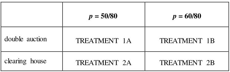
This experiment runs over 4 treatments. They crucially differ from one another in the market

institution (double auction/clearing house) and in the values we assign to the probabilities

p

and

q.

In table 1 we report the four possible combinations (treatments) we obtain by mixing the two

p

= 50/80

p

= 60/80

double auction

TREATMENT 1A

TREATMENT 1B

clearing house

TREATMENT 2A

TREATMENT 2B

Table 1: Treatments

On one hand, keeping the quantity of information (total number of signals) as a constant

parameter, moving from treatment 1 to treatment 2 we switch the trading institution. On the other

hand, moving from group A to group B treatments, we increase the likelihood for a signal to be

trusted. This latter feature leads to the following further consideratio ns.

While in the A treatments subjects receive the correct signal with a 63% chance, in B

treatments they receive the correct signal with a 75% chance.

2.3 Trading Institution

We should now describe the trading process. On one hand, we use a single-unit double-auction

mechanism, since it is well known from countless experiments (in simpler contexts) that this

mechanism can reach the competitive equilibrium quickly and efficiently. On the other hand, we

use a clearing house

–

in which subjects enter effectively a (price, quantity) pair which are then

aggregated to clear the market by the experimenter.

Note that, in both cases, agents can make losses. To avoid some of the problems associated

with subjects making real losses in experiments, we endowed all agents with a participation fee,

which could be used (if the subject agreed) to offset losses (all subjects which experienced losses

chose this option), or they can leave (none chose to leave). Subjects were informed that once this

participation fee was exhausted, any further losses had to be covered by the subjects themselves

–

but this case never happened in the experiment.

In a continuous double auction mechanism, each trader, at any moment during the trading

period, is free to enter a bid (an offer to buy one unit of the asset for a specific amount of cash) or

an ask (an offer to sell one unit of the asset for a specific amount of cash). When a trade proposal is

submitted, it appears on the book and it becomes public information. Traders can also accept

outstanding bids and/or asks. When an existing bid or ask is accepted by another trader, then a

1

We note that this is not the s ame as Goeree and Lindsay’s (2102b) schedule market, though it does have some features

transaction is completed and the price at which the contract has been closed also appears on the

book and becomes public information. Traders can buy/sell one unit at a time and as often as they

want (compatible with their budget constrain) in each trading period. Plott and Sunder (1982)

showed that a double auction trading mechanism performs particularly well in disseminating the

information, because it involves a continuous type of trading. In particular, each subject, while

trading, can observe the other traders

’

behaviours in the market. This feature produces the

information dissemination among traders. If the dissemination process is complete and immediate,

actual prices should reveal at any moment all the aggregate information in the market. However, in

the clearing house mechanism, each trader privately submits his purchase or sale order. For a single

unit of the asset, the purchase order consists of the highest acceptable purchase price and the sale

order represents the lowest acceptable sale price. When the trading (sub ) period closes, all the

orders previously submitted are collected and processed. In particular, purchase orders are ordered

from the highest to the lowest and the demand function is derived. Sale orders are ordered from the

lowest to the highest and the supply function is derived. The intersection point of the demand and

supply function determines the

clearing price

at which the orders will be executed. Nevertheless,

there is no guarantee that all the submitted orders will be executed. In particular, only the purchase

orders at a price equal to or above the clearing value and only the sale orders at a price equal to or

below the equilibrium value will be executed. Then, the clearing system provides the market with a

uniform price for each call. Typically, there could be more than one call per period. In our

experiment there are four calls in each trading period. In this kind of trading mechanism, each

trader, when submitting his proposal, cannot observe whether the other market participants are

operating as sellers or buyers and at which price they would like to sell or buy the asset. Only at the

end of each trading (sub) period does each trader observe the demand and supply functions and the

clearing price, realizing whether or not his proposal was executed. Therefore, in a call auction

system, a discrete type of time trading takes place.

In our particular framework, in the clearing house treatments, traders had the chance to

choose among three options: buying, selling or no-trading. If traders decided to be buyers (sellers)

they were asked to submit the price at which they would like to buy (sell) the asset and how many

units they would like to buy (sell) at that price. The state and the signal remained the same in the 4

sub-periods of each period. Only at the end of each period was the dividend revealed to the market

participants.

In the determination of the equilibrium price (clearing price), some particular cases can arise

in the clearing house

mechanism. In fact, traders’ orders can lead to situations in which there is an

the aggregate demand curve intersects with a horizontal segment of the aggregate supply curve. In

this case, there is an overlapping of quantities. Similarly, it may be that a vertical segment of the

aggregate demand curve intersects with a vertical segment of the aggregate supp ly curve. In this

case, there is an overlapping of prices. To explain how, in equilibrium, price and quantity are

determined in these special cases, first we report an example of quantities overlapping. Suppose that

6 subjects are trading in the market and that three of them are buyers and the other three are sellers.

Among the buyers, the first subject (subject 1) would like to buy 2 units at 17 ECU, the second

subject (subject 2) desires to buy 3 units at 15 ECU and the third subject (subject 3) wants to buy 2

units at 13 ECU. Among sellers, the first subject (subject 4) would like to sell 2 units at 11 ECU,

the second subject (subject 5) desires to sell 2 units at 15 ECU and the third subject (subject 6)

wants to buy 3 units at 16 ECU. The buyer and seller orders are summarized in table 2; the demand

and supply functions are drawn as in figure 1.

Demand side

Supply side

Buyer

Price

Quantity

Seller

Price

Quantity

Subject 1

17

2

Subject 4

11

2

Subject 2

15

3

Subject 5

15

2

Subject 3

13

2

Subject 6

16

3

Table 2

As we can see in figure 1, quantities overlap in the range from 2 to 4 units. The equilibrium

price is 15 ECU, where the demand and supply functions intersect. In this case, quantities are split

in the following way: the first buyer (subject 1) who offered to buy 2 units at 17 ECU will buy 2

units at 15 ECU, the second buyer (subject 2) who offered to buy 3 units at 15 ECU will buy only 2

units at 15 ECU. Subject 2 was not able to additionally buy the third unit because there were only

two units left at a price equal or below 15 ECU. The third buyer (subject 3) who offered to buy 2

units at 13 ECU bought no units because there were no units left at a price equal to or below 13

ECU. Similarly, the first seller (subject 4) who asked to sell 2 units at 11 ECU, sold 2 units at 15

ECU. The second seller (subject 5) who asked to sell 2 units at 15 ECU, sold 2 units at 15 ECU.

The third seller (subject 6) who asked to sell 3 units at 16 ECU did not buy anything because there

Figure 1

Second, we report an example where prices overlap. Suppose that 4 subjects are trading in

the market and that two of them are buyers and the other two are sellers. Among buyers, the first

subject (subject 1) would like to buy 2 units at 15 ECU and the second subject (subject 2) desires to

buy 2 units at 14 ECU. Among sellers, the first subject (subject 3) would like to sell 2 units at 10

ECU and the second subject (subject 4) desires to sell 2 units at 17 ECU.

Demand side

Supply side

Buyer

Price

Quantity

Seller

Price

Quantity

Subject 1

15

2

Subject 3

10

2

Subject 2

14

2

Subject 4

17

2

Table 3

Figure 2

The buyer and seller orders are summarized in table 2; the demand and supply functions are

The equilibrium quantity is unique and equal to 2 units. By definition, a competitive equilibrium

occurs at any price that equates the offered and demanded quantities. In this special case, the

demand and supply functions intersect along the vertical segment between 14 and 15. As a

consequence, any point on this vertical line is potentially a competitive price, which leads to the

same welfare. For concreteness, in cases with no-unique price solution, we compute the equilibrium

price as the mid-point of all the possible competitive prices. So, in this particular case, the

competitive price is assumed to be 14.5, which is the midpoint between 14 and 15. In particular, the

first buyer (subject 1), who offered to buy 2 units at 15 ECU, bought 2 units at 14.5 ECU and the

first seller (subject 3), who asked to sell 2 units at 10 ECU, sold 2 units at 14.5 ECU. Both the

second buyer (subject 2) and the second seller (subject 4) did not buy anything because their

proposals were respectively below and above the equilibrium price.

We will compare the two markets mechanisms in terms o f informational efficiency, standard

deviation and market volume. Friedman (1993) provides an early experimental study comparing the

double auction and the clearing house, though in the context of non- monetised trading. He

concludes that “clearinghouse

markets are as informationally efficient as double auction markets

and almost as allocationally

efficient”, while Cason and Friedman (2008) summarise a wealth of

experimental evidence by

saying that “price deviations from competitive equilibrium tend to be th

e

smallest with the SCM [clearing house], while volume is hi

ghest in CDA [double auction]”.

2.4 Earnings

At the beginning of each trading period, subjects start with their endowment of experimental money

and shares. During the trading process they can increase or decrease the number of units of the asset

that they own and, depending upon the prices at which they trade, their amount of experimental

money will increase or decrease during the period. At the end of each market period the dividend

value is announced and distributed in experimental money to the asset owners. Accordingly, at the

end of each trading period, agents will end up with a stock of experimental money which may be

more or less than that which they started that period with.

In any trading period, a

n agent’s trading profit is

computed as the difference between the

final stock of experimental money and the initial stock. For the experiment as a whole, the payment

to an agent is simply the sum of the profits over all the 7 real trading periods of the experiment.

Earnings were expressed in terms of Experimental Currency Units (ECU), which were

3

Experimental Results

In this section we present the experimental results derived from the comparison between the two

employed trading institutions. In particular, in line with the presented literature, our analysis has

been carried out taking into account price efficiency, market volume and market volatility. To begin

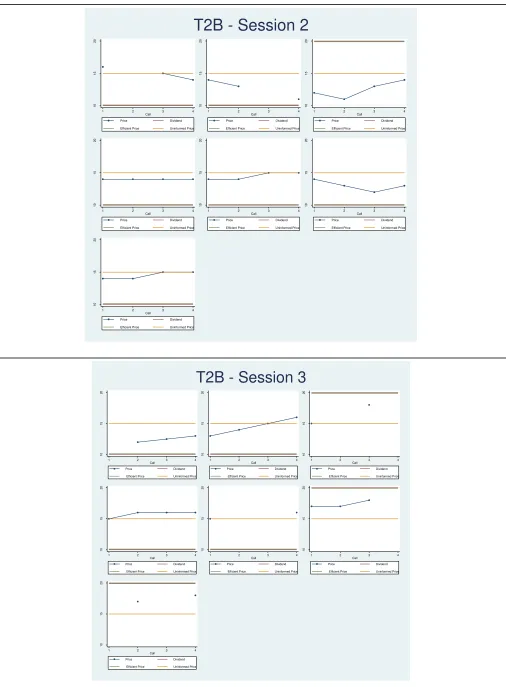
with, Figures B1 and B2 (Appendix B) show trading prices sub-divided by trading period (and

calls) in the double auction and clearing house treatments respectively. Price time series is

complemented with three benchmarks; i.e. the asset dividend, the expected value of the asset

(otherwise called “uninformed price”) and the “efficient price” (whose meaning and formulation

will be explained in the next lines). Furthermore, descriptive statistics are collected and reported in

Appendix C. In double auction treatments, market volume, mean and standard deviation of trading

prices are computed both over the entire trading period and at sub- intervals of 45 seconds each. In

clearing house treatments, since each call is cleared at a uniform price, market volume is computed

in each of the four calls and overall as a sum of the stocks traded in each call. Mean and standard

deviation of trading prices are computed over the whole trading period.

Price Efficiency

Following Vernon Smith (1962), we measure the accuracy of price discovery process by computing

the root mean square error between each of the

n

transaction prices

(for i=1…n)

over a given period

and the equilibrium price of that period, expressed as a percentage of the equilibrium price.

Substantially,

the Smith’s Alpha captures the standard deviation of actual prices over the theoretical

equilibrium value. Then, a lower value of this index is desirable, since it would imply that trading

prices exhibit smaller deviations from the market equilibrium price.





1 n

1 i

i

2

EP

TP

n

1

EP

1

SmithAlpha





















where:



EP

represents the equilibrium price;



TP

i

represents the actual price of transaction i;



n stands for the total number of transactions.

The challenging feature of our experimental design is in the fact that, in both treatments, no traders

know for sure the fundamental value of the asset. Depending on the treatment, at the start of each

62.5% (class A treatments) or 75% (class B treatments). Therefore, the fundamental value of the

asset is not a reliable proxy for testing market efficiency. Consequently, we resort to the concept of

“efficient price”

. We recall that the market is efficient if, at any instant of time, all the available

information is incorporated into trading prices. In our framework, this would mean that each agent

trades as if he or she knew both his or her signal

plus

other agents’ signal

as well. Through the use

of the Bayes rule principle, the efficient price formulation incorporates this inference process.

In particular, following Alfarano et al. (2015), we compute the efficient price as follows:

)

I

|

10

D

Pr(

10

)

I

|

20

D

Pr(

20

Price

Efficient













where I stands for the information set in a given trading period of a generic market. Recurring

to the Bayes rule, the probabilities that a certain dividend is realized conditional on the

market information set are defined as follows:

1

p

q

1

)

I

Pr(

)

20

D

Pr(

)

20

D

|

I

Pr(

)

I

|

20

D

Pr(











































q

p

1

)

I

|

20

D

Pr(

1

)

I

|

10

D

Pr(









































.

with:

X

x

2







where:



p is the probability that a single private signal is correct;



q = 1

−

p is the probability that a single private signal is incorrect;



x

is the number of

“20”

signals in a given market;



X

is the total number of signals in a given market.

Following the efficient price formulation, in class A treatments (where 5 correct signals are

exogenously and ex-ante injected in the market) the efficient price is equal to 17.35 ECU in periods

where the good state (Dividend 20) is the realized one and to 12.65 ECU in periods where the bad

state (Dividend 10) occurs. In class B treatments (where 6 correct signals are exogenously and

ex-ante injected in the market) the efficient price is equal to 19.88 ECU and 10.12 ECU in good and

bad states respectively. These values constitute the benchmarks against which actual prices are

As a main contribution, the overall market efficiency is investigated by comparing the two

trading institutions regardless of the number of correct signals in the market; i.e. for each trading

institutions, aggregating data from class A and class B treatments. Figure 3 shows the box-plot of

the call market and double auction Smith’s Alpha distribution

s computed on the efficient price. The

double auction distribution is visibly downward shifted with respect to the call market one,

implying that a closer benchmark tracking is detected when trading is conducted through the double

auction rules. A non-parametric two-sided Mann-Whitney U test shows that this achievement is

statistically significant (z = 2.51, p = 0.0119).

Figure 3: Efficient Price Smith’s Alpha

A closer inspection has been carried out performing pairwise comparisons of treatments. The

following results

have been achieved. While the double auction performs better than the call

market when only five correct signals are in the market (z = -2.578, p = 0.0099), the two trading

institutions provide a similar level of informational efficiency when six correct signals are in the

market. One possible explanation for this achievement might be in the fact that, when there is

“enough” trustable information in the market, the adopted trading institution does not play a major

role in promoting the price discovery. Very interestingly, double auction markets with only five

correct signals outperform clearing house markets with six correct signals ( z = -2.126, p = 0.0335).

In line with this last evidence, the informational efficiency of double auction markets with six

correct signals is higher than that of call markets with five correct signals (z = -2.050, p = 0.0403).

In clearing house markets, a significant improvement in informational efficiency is detected when

moving from five to six correct signals in the market. Surprisingly, double auction markets with

five correct signals stimulate higher efficiency than double auction markets with six correct signals.

2

Box-Plots and statistical tests are available in Appendix D

0

.5

1

1

.5

2

Result 1: In several instances, the double auction institution promotes higher informational

efficiency than the call market one.

Volatility

Figure 4 presents price volatility grouped by treatment, and measured in terms of standard deviation

of trading prices. Figure G1 (Appendix G) provides further grouping by session. Overall, we find

that clearing house markets promote lower average volatility than double auction markets but this

achievement is not statistically significant

.

Figure 4: Average standard deviation of trading prices

A pairwise comparison between T1A and T2A, as well as between T1B and T2B show that clearing

house markets reduce the average price volatility, keeping constant the number of correct signals in

the market. Nevertheless, our results

report that this evidence is not statistically significant. The

only significant achievements show that double auction markets with 5 correct signals exhibit lower

volatility than double auction markets with 6 correct signals and that clearing house markets with

five correct signals promote lower volatility than double auction markets with six correct signals.

Result 2: None of the two employed trading institutions is superior in te rms of promoting

lower volatility of actual prices

3

A non-parametric two-sided Mann-Whitney U test shows that this achievement is statistically significant (z = -1.34, p = 0.2569).

4

Statistical tests are reported in Appendix E

0

.5

1

1

.5

Market Volume

Contrarily to the theoretical prediction of the No-Trade theorem by Milgrom and Stokey (1982), our

experimental evidence shows that sustained trading occurred in all markets. Figure 5 reports market

volume grouped by treatment and measured as number of traded stocks. Figure G2 (Appendix G)

shows further grouping by session. Putting together data from treatments 1A and 1B (i.e.

considering market volume in double auction markets), as well as data from treatments 2A and 2B

(i.e. considering market volume in call auction markets), we find no significant differences in

market volume between the two trading institutions

.

Figure 5:

Keeping equal the number of correct signals in the market, a decrease in market volume is observed

when switching from double auction to call auction markets, i.e. moving from T1A to T2A and

from T1B to T2B. Anyway, in both the case this reduction in volume is not significant

. The

remaining pairwise comparisons over treatments lead to significant results. Indeed, being equal the

adopted trading institution, an increase in the number of correct signals (i.e. moving from T1A to

T1B and from T2A to T2B) does significantly reduce market volume. Finally, call auction markets

with six correct signals exhibit lower volume than double auction markets with five correct signals

(see comparison T1A vs. T2B) and double auction markets with 6 correct signals promote lower

volume than call markets with five correct signals (see comparison T1B vs. T2A).

5

A non-parametric two-sided Mann-Whitney U test shows that this achievement is statistically significant (z = -0.663, p = 0.5076).

6

Statistical tests on market volume are reported in reported in Appendix F

0

10

20

30

40

Result 3: Double auction and call auction markets do not exhibit significantly dive rse market

volume. Within a trading institution, an increase in the numbe r of correct signals generates

lower volume.

4.

Conclusion

In this paper we have compared, by mean of a lab experiment, two market institution: the double

auction and the clearing house. One clear message emerges from this experiment: the observed

price converge faster to the equilibrium when the trading institution is the double auction. To be

more precise in this experiment we compare the two market institutions in terms of price efficiency,

market volume and market volatility.

Concerning price efficiency, we first compared the two trading institutions regardless of the

information present in the markets, under low and high information precision. The double auction

distribution is downward shifted with respect to the clearing house one, implying that a closer

benchmark tracking is detected when trading is conducted through the double auction rules. More

precisely, on one hand, contrary to Friedman (1993) the double auction performs better than the

clearing house when information precision in the market is low; on the other hand, accordingly to

Friedman (1993) when information precision in the market is high, the two market mechanisms are

not statistically different. Very interestingly, double auction markets with poor information

outperform clearing house markets with abundant information.

Regarding Market Volatility

–

accordingly to Friedman (1993)

–

we found that clearing house

markets promote lower average volatility than double auction markets, but this achievement is not

statistically significant. Also comparing the two market mechanisms under low and high

information precision environments show that clearing house markets reduce the average price

volatility, but the reduction in volatility is not statistically significant. Concerning market volatility

we can state that none of the two employed trading institutions is superior in terms of promoting

lower volatility of actual prices

Observing Market Volume

–

accordingly to Friedman (1993)

–

we found no significant

differences between the two market institutions. Comparing the two market mechanisms in low and

high information precision environments a decrease in market volume is observed when switching

from double auction to clearing house. Anyway, this reduction in volume is not significant.

Concerning market volume double auction and call auction markets do not exhibit statistically

significantly difference.

We can conclude that the double auction mechanism is better then the clearing market in

References

Alfarano, Simone, Eva Camacho, and Andrea Morone (2011) The role of public and private

information in a laboratory financial market. IVIE.

Angrisani, Marco, Antonio Guarino, Steffen Huck and Nathan C. Larson (2011) No-Trade in the

Laboratory.

The B.E. Journal of Theoretical Economics, 11(1), 1-58.

Bachelier, Louis (1900) Théorie de la spéculation. Gauthier-Villars.

Banerjee, Abhijit V. (1992) A simple model of herd behavior. The Quarterly Journal of Economics

797-817.

Bikhchandani, Sushil, David Hirshleifer, and Ivo Welch (1992) A theory of fads, fashion, custom,

and cultural change as informational cascades.

Journal of political Economy 992-1026.

Cason, Timothy N., and Daniel Friedman (1996) Price formation in double auction markets.

Journal of Economic Dynamics and Control 20(8), 1307-1337.

Cason, Timothy N., and Daniel Friedman (1997) Price formation in single call markets.

Econometrica, 311-345.

Cason, Timothy, and Daniel Friedman (1999) Price formation and exchange in thin markets: A

laboratory comparison of institutions. Money, Markets, and Method: Essays in Honour of

Robert W. Clower 155-179.

Easley, David, and John Ledyard (1993) Theories of price formation and exchange in double oral

auctions. The double auction market: Institutions, theories, and evidence 15.

Fama, Eugene F. (1965) The behavior of stock-market prices.

Journal of business, 34-105.

Fama, Eugene F. (1970) Efficient capital markets: A review of theory and empirical work.

The

journal of Finance 25(2), 383-417.

Fama, Eugene F. (1991) Efficient capital markets: II. The journal of finance, 46(5), 1575-1617.

Fama, Eugene F. (1998) Market efficiency, long-term returns, and behavioral finance.

Journal of

financial economics 49(3), 283-306.

Fischbacher, Urs (2007) z-Tree: Zurich toolbox for ready-made economic experiments.

Experimental Economics 10(2), 171-178.

Fiore, Annamaria, and Andrea Morone (2008) A Simple Note on Informational Cascades

Economics - The Open-Access, Open-Assessment E-Journal, 2, 1-21.

Friedman, Daniel (1984) On the Efficiency of Experimental Double Auction Markets.

American

Economic Review

, 74(1), 60-72.

Friedman, Daniel (1993) How trading institutions affect financial market performance: Some

Hey, John D. and Andrea Morone (2004) Do markets drive out lemmings

—

or vice versa?.

Economica 71(284): 637-659.

Hinterleitner, Gernot, U. Leopold-Wildburger, Roland Mestel, and Stefan Palan (2015) A Good

Beginning Makes a Good Market: The Effect of Different Market Opening Structures on

Market Quality.

The Scientific World Journal

.

Morone, Andrea (2008) Financial markets in the laboratory: an experimental analysis of some

stylized facts.

Quantitative Finance 8(5), 513-532.

Morone, Andrea (2012) A simple model of herd behavior, a comment. Economics Letters, 114(2),

208-211.

Morone, Andrea and Simone Nuzzo (2016) Asset markets in the lab: a literature review. Mimeo

Morone, Andrea and Eleni Samanidou (2008) A simple note on herd behaviour.

Journal of

Evolutionary Economics, 18(5), 639-646.

Morone, Andrea, Serena Sandri, and Annamaria Fiore (2009) On the absorbability of informational

cascades in the laboratory.

Journal of Behavioral and Experimental Economics 38(5),

728-738.

Noussair, Charles N., and Steven Tucker (2013) Experimental research on asset pricing.

Journal of

Economic Surveys

27.3, 554-569

Palan, Stefan (2013) A review of bubbles and crashes in experimental asset markets.

Journal of

Economic Surveys

27.3, 570-588.

Plott, Charles R. (2000) Markets as information gathering tools. Southern Economic Journal 67(1):

2-15.

Powell, Owen, and Natalia Shestakovaa, (2016) Experimental asset markets: A survey of recent

developments.

Journal of Behavioral and Experimental Finance 12, 14–22

Schnitzlein, C.R. (1996) Call and continuous trading mechanisms under asymmetric information:

an experimental investigation.

Journal of Finance

51, 613-636.

Smith, Vernon L., Arlington W. Williams (1982) An experimental comparison of alternative rules

for competitive market exchange, in: Engelbrecht-Wiggans, R., Shubik, M., Stark, R. (Eds.)

Auctions, Bidding and Contracting: Uses and Theory. New York University Press, New

York, pp. 172-200.

Theissen, E. (2000) Market structure, informational efficiency and liquidity. An experimental

Appendix A: Instrucciones

Treatment 1A

Bienvenidos al experimento

En este experimento, se te pedirá que tomes decisiones en un mercado financiero. El experimento es sencillo y las instrucciones son fáciles de entender. Si las sigues cuidadosamente, puedes ganar una cantidad considerable de dinero que se te pagará en efectivo al final del experimento.

Presentación del experimento

Este experimento se basa en un mercado, compuesto por diferentes períodos de intercambio. En este mercado sólo hay un tipo de bien, que llamaremos "acción", que se intercambia. En cualquier mo ment o durante cada período de intercambio, tu puedes comprar y/o vender las acciones. La moneda en la que se negocian las acciones se llama "ECU". Tu pago en efectivo al final del experimento será en Euros. La tasa de conversión será igual a 1 euro cada 75 "EC U". Durante este experimento se puede ganar tanto de la venta de las acciones como de los dividendos de las mismas acciones.

Instrucciones Generales

El mercado se compone de 8 participantes y diferentes períodos de intercambio, unos son de prueba y unos re ales. Los periodos de prueba serán útiles para comprender el funcionamiento del programa informático. En los periodos de prueba, no se te pagará por tus ganancias. Sólo los períodos reales se tendrán en cuenta para el cálculo de tus ganancias. Al principio de cada período de intercambio recib irás una dotación de 2.000 ECU y 10 acciones. Al final de cada periodo de intercambio, cada una de las acciones pagará un dividendo de 10 o 20. El valor del d ividendo, al emp iece de cada período se determinará al azar y no será revelado a los participantes. Más precisamente, con una probabilidad del 50%, el dividendo será 10 y con una probabilidad del 50% el dividendo será 20.

Al princip io de cada período de intercambio, en el mercado habrán 80 señales de información sob re el valor del dividendo. De estas 80 señales de información, 50 serán correctas y 30 incorrectas. Según una regla completamente aleatoria, en cada período, cada sujeto recibirá una de las ochenta señales presentes en el mercado. Por lo tanto, existe una probabilidad del 63% (50/80) de que tu recibas la señal correcta y una probabilidad del 37% (30/ 80) de que recibas la señal incorrecta.

Por ejemplo, si el valor extraído del dividendo es igual a 20, con un 63% de probabilidad recibirás una señal que te indica que el dividendo es 20 (señal correcta) y con un 37% de probabilidad recibirás una señal que te indica que el dividendo es 10 (señal incorrecta). Del mismo modo, si el valor extraído del dividendo es igual a 10, con un 63% de probabilidad recib irás una señal que te indica que el dividendo es 10 (señal co rrecta) y con un 37% de probabilidad recibirás una señal que te indica que el dividendo es 20 (señal incorrecta).

Negociación

Figura 5: Mercado

Podrás participar en las siguientes cuatros formas:

1. For mul ando una oferta de venta de la acción, introduciendo el preci o al que estás dispuesto a ve nder.

Para formu lar una oferta de venta, tienes que introducir el precio al que deseas vender en el cuadro " Introduce aquí tu oferta de venta" en la primera colu mna a la izquierda de la pantalla; a continuación, haz clic en "Envías al mercado tu oferta de venta" en la misma colu mna. En la segunda columna a la derecha podrás ver la lista de las ofertas presentadas por los diferentes participantes. La oferta de venta más baja, siempre se colocará al final de la lista. Tu oferta de venta se mostrará en azul.

2. For mul ando una oferta de compra de la acci ón, introduciendo el precio al que estás dispuesto a compr ar. Para formu lar una oferta de co mpra, t ienes que introducir el precio al que deseas comprar en el cuadro " Introduce aquí tu oferta de co mpra" en la primera colu mna a la derecha de la pantalla, luego, haz clic en " Envías al mercado tu oferta de compra" a continuación en la misma colu mna. La segunda columna de la izquierda muestra una lista de ofertas presentadas por los diferentes participantes. La o ferta de co mpra más alta siempre se colocará en la parte inferior de la lista. Tu oferta de compra se mostrará en azul.

3. Vender una acci ón me diante la ace ptación de una oferta de c ompr a. Puedes seleccionar una oferta de compra de la segunda columna de la izquierda, haciendo clic en él. A l hacer clic en el botón " Vende" al fondo de la mis ma co lu mna, estarás vendiendo una acción al precio indicado. No puedes vender acciones a ti mismo. Cuando aceptas una oferta de compra, la mis ma desaparecerá de la lista. Si has enviado previamente al mercado una oferta de venta, la mis ma oferta desaparecerá de la lista de ofertas de venta porque ya has vendido la acción.

4. Comprar una acción, ace ptando una oferta de ve nta. Puedes seleccionar una oferta de venta de la segunda columna a la derecha haciendo clic en ella. Al hacer clic en el botón "Compra" al fondo de la mis ma colu mna, estarás comprando una acción al precio indicado. No puedes comprar acciones de ti mis mo. Cuando aceptas una oferta de venta, la misma desaparecerá de la lista. Si has enviado previamente al mercado una oferta de compra, la misma desaparecerá de la lista de ofertas de compra, porque ya has comprado la acción.

Cada vez que aceptas una oferta de venta o de co mpra un nuevo contrato se ha cerrado y su precio aparece en la columna "Precios de negociación ".

Tus ganancias

Co mo se muestra en la Figura 6, al final de cada período, tus ganancias serán iguales a "Moneda antes de cobrar el dividendo" menos "Moneda inicial" más "Dividendo Total".

Figura 6: Tus ingresos en el período

Tu ganancia total del experimento será la suma de tus ingresos en cada uno de los 7 períodos "reales".

El siguiente esquema muestra el desglose de tus ganancias en cada período de negociación

1. Moneda – (Nº de acciones compradas x el precio de compra) + (Nº de acciones vendidas x el precio de venta)

= Moneda antes de cobrar el dividendo

2. Dividendo del período x (Nº de acciones al final del período) = Dividendo total

3. Moneda antes de cobrar el dividendo – Moneda inicial + Dividendo total = Ganancia total (al final del

período) 4.

Treatment 1B

Bienvenidos al experimento

En este experimento, se te pedirá que tomes decisiones en un mercado financiero. El experimento es sencillo y las instrucciones son fáciles de entender. Si las sigues cuidadosamente, puedes ganar una cantidad considerable de dinero que se te pagará en efectivo al final del experimento.

Presentación del experimento

Este experimento se basa en un mercado, compuesto por diferentes períodos de intercambio. En este mercado sólo hay un tipo de bien, que llamaremos "acción", que se intercambia. En cualquier mo mento durante cada período de intercambio, tu puedes comprar y/o vender las acciones. La moneda en la que se negocian las acciones se llama "ECU". Tu pago en efectivo al final del experimento será en Euros. La tasa de conversión será igual a 1 euro cada 75 "ECU". Durante este experimento se puede ganar tanto de la venta de las acciones como de los dividendos de las mismas acciones.

Instrucciones Generales

El mercado se compone de 8 participantes y diferentes períodos de intercambio, unos son de prueba y unos reales. Los periodos de prueba serán útiles para comprender el funcionamiento del p rograma informático. En los periodos de prueba, no se te pagará por tus ganancias. Sólo los períodos reales se tendrán en cuenta para el cálculo de tus ganancias. Al principio de cada período de intercambio recib irás una dotación de 2.000 ECU y 10 acciones . Al final de cada periodo de intercambio, cada una de las acciones pagará un dividendo de 10 o 20. El valor del d ividendo, al emp iece de cada período se determinará al azar y no será revelado a los participantes. Más precisamente, con una probabilidad del 50%, el dividendo será 10 y con una probabilidad del 50% el dividendo será 20.

Al princip io de cada período de intercambio, en el mercado habrán 80 señales de información sobre el valor del dividendo. De estas 80 señales de información, 60 serán correctas y 20 incorrectas. Según una regla completamente aleatoria, en cada período, cada sujeto recibirá una de las ochenta señales presentes en el mercado. Por lo tanto, existe una probabilidad del 75% (60/80) de que tu recibas la señal correcta y una probabilid ad del 25% (20/ 80) de que recibas la señal incorrecta.

Por ejemplo, si el valor extraído del dividendo es igual a 20, con un 75% de probabilidad recibirás una señal que te indica que el dividendo es 20 (señal correcta) y con un 25% de probabilidad recibirás una señal que te indica que el dividendo es 10 (señal incorrecta). Del mismo modo, si el valor extraído del dividendo es igual a 10, con un 75% de probabilidad recib irás una señal que te indica que el dividendo es 10 (señal co rrecta) y con un 25% de pr obabilidad recibirás una señal que te indica que el dividendo es 20 (señal incorrecta).

Negociación

Figura 5: Mercado

Podrás participar en las siguientes cuatros formas:

5. For mul ando una oferta de venta de la acción, introduciendo el preci o al que estás dispuesto a ve nder.

Para formu lar una oferta de venta, tienes que introducir el precio al que deseas vender en el cuadro " Introduce aquí tu oferta de venta" en la primera colu mna a la izquierda de la pantalla; a continuación, haz clic en "Envías al mercado tu oferta de venta" en la misma colu mna. En la segunda columna a la derecha podrás ver la lista de las ofertas presentadas por los diferentes participantes. La oferta de venta más baja, siempre se colocará al final de la lista. Tu oferta de venta se mostrará en azul.

6. For mul ando una oferta de compra de la acci ón, introduciendo el precio al que estás dispuesto a compr ar. Para formu lar una oferta de co mpra, t ienes que introducir el precio al que deseas comprar en el cuadro " Introduce aquí tu oferta de co mpra" en la primera colu mna a la derecha de la pantalla, luego, haz clic en " Envías al mercado tu oferta de compra" a continuación en la misma colu mna. La segunda columna de la izquierda muestra una lista de ofertas presentadas por los diferentes participantes. La o ferta de co mpra más alta siempre se colocará en la parte inferior de la lista. Tu oferta de compra se mostrará en azul.

7. Vender una acci ón me diante la ace ptación de una oferta de c ompr a. Puedes seleccionar una oferta de compra de la segunda columna de la izquierda, haciendo clic en él. A l hacer clic en el botón " Vende" al fondo de la mis ma co lu mna, estarás vendiendo una acción al precio indicado. No puedes vender acciones a ti mismo. Cuando aceptas una oferta de compra, la mis ma desaparecerá de la lista. Si has envia do previamente al mercado una oferta de venta, la mis ma oferta desaparecerá de la lista de ofertas de venta porque ya has vendido la acción.

8. Comprar una acción, ace ptando una oferta de ve nta. Puedes seleccionar una oferta de venta de la segunda columna a la derecha haciendo clic en ella. Al hacer clic en el botón "Compra" al fondo de la mis ma colu mna, estarás comprando una acción al precio indicado. No puedes comprar acciones de ti mis mo. Cuando aceptas una oferta de venta, la misma desaparecerá de la lista. Si has enviado previamente al mercado una oferta de compra, la misma desaparecerá de la lista de ofertas de compra, porque ya has comprado la acción.

la colu mna central de la pantalla, "Precios de negociación ", podrás ver los precios a los que las acciones se negocian en el período actual.

Cada vez que aceptas una oferta de venta o de co mpra un nuevo contrato se ha cerrado y su precio aparece en la columna "Precios de negociación ".

Tus ganancias

Co mo se muestra en la Figura 6, al final de cada período, tus ganancias serán iguales a "Moneda antes de cobrar el dividendo" menos "Moneda inicial" más "Dividendo Total".

Figura 6: Tus ingresos en el período

Tu ganancia total del experimento será la suma de tus ingresos en cada uno de los 7 períodos "reales".

El siguiente esquema muestra el desglose de tus ganancias en cada período de negociación

5. Moneda – (Nº de acciones compradas x el precio de compra) + (Nº de accio nes vendidas x el precio de venta)

= Moneda antes de cobrar el dividendo

6. Dividendo del período x (Nº de acciones al final del período) = Dividendo total

7. Moneda antes de cobrar el dividendo – Moneda inicial + Dividendo total = Ganancia total (al final del

período)

Treatment 2A

Bienvenidos al experimento

En este experimento, se te pedirá que tomes decisiones en un mercado financiero. El experimento es sencillo y las instrucciones son fáciles de entender. Si las sigues cuidadosamente, puedes ganar una cantidad considerable de dinero que se te pagará en efectivo al final del experimento.

Presentación del experimento

Este experimento se basa en un mercado, compuesto por diferentes períodos de intercambio. En este me rcado sólo hay un tipo de bien, que llamaremos "acción", que se intercambia. En cualquier mo mento durante cada período de intercambio, tu puedes comprar y/o vender las acciones. La moneda en la que se negocian las acciones se llama "ECU". Tu pago en efectivo al final del experimento será en Euros. La tasa de conversión será igual a 1 euro cada 75 "ECU". Durante este experimento se puede ganar tanto de la venta de las acciones como de los dividendos de las mismas acciones.

Instrucciones Generales

El mercado se compone de 8 participantes y diferentes períodos de intercambio, unos son de prueba y unos reales. Los periodos de prueba serán útiles para comprender el funcionamiento del programa informático. En los periodos de prueba, no se te pagará por tus ganancias. Sólo los períodos reales se tendrán en cuenta para el cálculo de tus ganancias. Al principio de cada período de intercambio recib irás una dotación de 2.000 ECU y 10 acciones. Al final de cada periodo de intercambio, cada una de las acciones pagará un d ividendo de 10 o 20. El valor del d ividendo, al emp iece de cada período se determinará al azar y no será revelado a los participantes. Más precisamente, con una probabilidad del 50%, el dividendo será 10 y con una probabilidad del 50% el dividendo será 20.

Al princip io de cada período de intercambio, en el mercado habrán 80 señales de información sobre el valor del dividendo. De estas 80 señales de información, 50 serán correctas y 30 incorrectas. Según una regla completamente aleatoria, en cada período, cada sujeto recibirá una de las ochenta señales presentes en el mercado. Por lo tanto, existe una probabilidad del 63% (50/80) de que tu recibas la señal correcta y una probabilidad del 37% (30/ 80) de que recibas la señal incorrecta.

Por ejemplo, si el valor extraído del dividendo es igual a 20, con un 63% de probabilidad recibirás una señal que te indica que el dividendo es 20 (señal correcta) y con un 37% de probabilidad recibirás una señal que te indica que el dividendo es 10 (señal incorrecta). Del mismo modo, si el valor extraído del dividendo es igual a 10, con un 63% de probabilidad recib irás una señal que te indica que el dividendo es 10 (señal co rrecta) y con un 37% de probabilidad recibirás una señal que te indica que el dividendo es 20 (señal incorrecta).

Negociación

El mercado se compone de 9 períodos de intercambio, de los cuales 2 de prueba y 7 reales. Cada período de intercamb io se divide en cuatro sub-períodos. Cada sub-período tendrá una duración de 60 segundos. El valor del div idendo extraído seguirá siendo el mis mo para los 4 sub-períodos que componen el período. La señal recibida seguirá siendo la mis ma para los 4 sub-períodos que componen el período.

Al co mienzo de cada sub-periodo (Figura 1), el programa informát ico te enseñará en la parte superior izquierda, el período y el sub-período en el que la negociación se está llevando a cabo y en la parte superior derecha el t iempo restante (en segundos) antes el cierre del sub-período.

En la segunda línea en el panel izquierdo, la pantalla muestra tu cantidad total de dinero disponible y el número de tus acciones, en el panel derecho de la pantalla se te enseñará tu señal.

Figura 1: Métodos de negociación

En concreto, en cada sub-período puedes tomar las tres decisiones siguientes (panel grande de Figura 1):

1. Vender acciones

2. Comprar acciones

3. No participar a la negociación

Figura 2: Quiero ser vendedor

Además de los parámetros generales descritos anteriormente ( moneda, nú mero de acciones, tiempo disponible y señal), esta pantalla mostrará, en la segunda línea en la parte superior izquierda, tu posición de " Vendedor". En la parte central de la pantalla, se te pedirá que introduzca el precio de venta y el número de acciones que te gustaría vender a ese precio. El mis mo procedimiento se seguirá en caso de que decidas comprar. En ese caso, la pantalla mostrará, en la segunda línea en la parte superior izquierda, la posición de "Co mprador". En la parte principal de la pantalla, se te pedirá que introduzca el p recio de co mpra y el nú mero de acciones que desea comprar a ese precio. Por últ imo, si decides por la opción "No quiero intercambiar", no to maras parte en la negociación. Por lo tanto la cantidad de dinero y el nú mero de acciones de tu propiedad no van a cambiar.

En este mercado, tus pedidos de venta y de comp ra representan sólo una propuesta y no hay ninguna garantía de que tus pedidos se ejecutarán. La ejecución de los pedidos depende de lo siguiente.

Figura 3: demanda y oferta

Tras la determinación del precio de equilibrio, sólo si tu orden de venta será ejecutado (es decir, si habías

propuesto un precio de venta igual o menor que el precio de equilibrio), el nú mero de tus acciones se disminuirá del número de acciones que ofreciste vender y el dinero a tu d isposición se incrementará en una cantidad igual al número d e acciones vendidas multiplicado por el precio de venta (es decir, el precio de equilibrio) de cada acción.

Tras la determinación del precio de equilibrio, sólo si tu orden de co mpra será ejecutado (es decir, si ofreciste un precio de compra igual o mayor que el precio de equilibrio), el número de acciones en tu cartera aumentará el número de acciones que propusiste comprar y el dinero a tu d isposición se reducirá por un impo rte igual al número de acciones compradas, multiplicado por el precio de compra (es decir, el precio de equilibrio) de cada acción.

Tus ganancias

Al final de cada sub-período recibirás una información actualizada sobre tu actividad en el sub -período. La actualización inclu irá el nú mero de acciones y el dinero al principio del sub-periodo, tu pedido de compra o venta con su precio, número de acciones compradas o vendidas con su precio de ejecución del pedidos, número de acciones y el resto del dinero que te queda. Además de estas informaciones, tal co mo se muestra en el Figura 4, sólo en el ú ltimo sub-período de cada sub-período (es decir, al final de cada sub-período), se te dará a conocer el valor del d ividendo y la ganancia total del período.

Figura 4: Ganancia el último sub-período del período

Treatment 2B

Bienvenidos al experimento

En este experimento, se te pedirá que tomes decisiones en un mercado financiero. El experimento es sencillo y las instrucciones son fáciles de entender. Si las sigues cuidadosamente, puedes ganar una cantidad considerable de dinero que se te pagará en efectivo al final del experimento.

Presentación del experimento

Este experimento se basa en un mercado, compuesto por diferentes períodos de intercambio. En e ste mercado sólo hay un tipo de bien, que llamaremos "acción", que se intercambia. En cualquier mo mento durante cada período de intercambio, tu puedes comprar y/o vender las acciones. La moneda en la que se negocian las acciones se llama "ECU". Tu pago en efectivo al final del experimento será en Euros. La tasa de conversión será igual a 1 euro cada 75 "ECU". Durante este experimento se puede ganar tanto de la venta de las acciones como de los dividendos de las mismas acciones.

Instrucciones Generales

Al princip io de cada período de intercambio, en el mercado habrán 80 señales de información sobre el valor del dividendo. De estas 80 señales de información, 60 serán correctas y 20 incorrectas. Según una regla completamente aleatoria, en cada período, cada sujeto recibirá una de las ochenta señales presentes en el mercado. Por lo tanto, existe una probabilidad del 75% (60/80) de que tu recibas la señal correcta y una probabilidad del 25% (20/ 80) de que recibas la señal incorrecta.

Por ejemplo, si e l valor extraído del dividendo es igual a 20, con un 75% de probabilidad recibirás una señal que te indica que el dividendo es 20 (señal correcta) y con un 25% de probabilidad recibirás una señal que te indica que el dividendo es 10 (señal incorrecta). Del mismo modo, si el valor extraído del dividendo es igual a 10, con un 75% de probabilidad recib irás una señal que te indica que el dividendo es 10 (señal co rrecta) y con un 25% de probabilidad recibirás una señal que te indica que el dividendo es 20 (señal incorrecta).

Negociación

El mercado se compone de 9 períodos de intercambio, de los cuales 2 de prueba y 7 reales. Cada período de intercamb io se divide en cuatro sub-períodos. Cada sub-período tendrá una duración de 60 segundos. El valor del div idendo extraído seguirá siendo el mis mo para los 4 sub-períodos que componen el período. La señal recibida seguirá siendo la mis ma para los 4 sub-períodos que componen el período.

Al co mienzo de cada sub-periodo (Figura 1), el programa informát ico te enseñará en la parte superior izquierda, el período y el sub-período en el que la negociación se está llevando a cabo y en la parte superior derecha el t iempo restante (en segundos) antes el cierre del sub-período.

En la segunda línea en el panel izquierdo, la pantalla muestra tu cantidad total de dinero disponible y el número de tus acciones, en el panel derecho de la pantalla se te enseñará tu señal.

En el panel grande te enseñará el conjunto de tus opciones.

Figura 1: Métodos de negociación

1. Vender acciones

2. Comprar acciones

3. No participar a la negociación

Si decides vender o comprar acciones, la siguiente pantalla te preguntará a que precio quieres vender o comprar acciones y el número de acciones que deseas vender o comprar. Por ejemp lo, si decides vender acciones, se te entra la siguiente pantalla (Figura 2):

Figura 2: Quiero ser vendedor

Además de los parámetros generales descritos anteriormente (moneda, nú mero de acciones, tiempo disponible y señal), esta pantalla mostrará, en la segunda línea en la parte superior izquierda, tu posición de " Vendedor". En la parte central de la pantalla, se te pedirá que introduzca el precio de venta y el número de acciones que te gustaría vender a ese precio. El mis mo procedimiento se seguirá en caso de que decidas comprar. En ese caso, la pantalla mostrará, en la segunda línea en la parte superior izquierda, la posición de "Co mprador". En la parte principal de la pantalla, se te pedirá que introduzca el p recio de co mpra y el nú mero de acciones que desea comprar a ese precio. Por últ imo, si decides por la opción "No quiero intercambiar", no to maras parte en la negociación. Por lo tanto la cantidad de dinero y el nú mero de acciones de tu propiedad no van a cambiar.

En este mercado, tus pedidos de venta y de comp ra representan sólo una propuesta y no hay ninguna garantía de que tus pedidos se ejecutarán. La ejecución de los pedidos depende de lo siguiente.

sólo las órdenes de compra a un precio igual o mayor que el precio de equilibrio se realizarán así como sólo se realizarán las órdenes de venta a un precio igual o por debajo del precio de equilibrio.

Figura 3: demanda y oferta

Tras la determinación del precio de equilibrio, sólo si tu orden de venta será ejecutado (es decir, si habías

propuesto un precio de venta igual o menor que el precio de equilibrio), el nú mero de tus acciones se disminuirá del número de acciones que ofreciste vender y el dinero a tu d isposición se incrementará en una cantidad igual al número d e acciones vendidas multiplicado por el precio de venta (es decir, el precio de equilibrio) de cada acción.

Tras la determinación del precio de equilibrio, sólo si tu orden de co mpra será ejecutado (es decir, si ofreciste un precio de compra igual o mayor que el precio de equilibrio), el número de acciones en tu cartera aumentará el número de acciones que propusiste comprar y el dinero a tu d isposición se reducirá por un impo rte igual al número de acciones compradas, multiplicado por el precio de compra (es decir, el precio de equilibrio) de cada acción.

Tus ganancias

Al final de cada sub-período recibirás una información actualizada sobre tu actividad en el sub -período. La actualización inclu irá el nú mero de acciones y el dinero al principio del sub -periodo, tu pedido de compra o venta con su precio, número de acciones compradas o vendidas con su precio de ejecución del pedidos, número de acciones y el resto del dinero que te queda. Además de estas informacione