Munich Personal RePEc Archive
A Nonparametric Option Pricing Model
Using Higher Moments
Cayton, Peter Julian
Research School of Finance, Actuarial Studies, and Applied
Statistics, College of Business and Economics, The Australian
National University, School of Statistics, University of the
Philippines Diliman
April 2015
Online at
https://mpra.ub.uni-muenchen.de/63755/
A Nonparametric Option Pricing Model Using
Higher Moments
Peter Julian Cayton
∗April 20, 2015
Abstract
A nonparametric model that includes non-Gaussian characteristics of
skewness and kurtosis is proposed based on the cubic market capital asset
pricing model. It is an equilibrium pricing model but risk-neutral
valua-tion can be introduced through return data transformavalua-tion. The model
complies with the put-call parity principle of option pricing theory. The
properties of the model are studied through simulation methods and
com-pared with the Black-Scholes model. Simulation scenarios include cases on
nonnormality in skewness and kurtosis, nonconstant variance, moneyness,
contract duration, and interest rate levels. The proposed model can have
negative prices in cases of out-of-money options and in simulation cases
that are different from real-market situations, but the frequency of
neg-ative prices is reduced when risk-neutral valuation is implemented. The
model is more adaptive and more conservative in pricing options compared
to the Black-Scholes model when nonnormalities exist in the returns data.
1
Introduction
The paper proposes a nonparametric option pricing model that accounts for
higher-moment features of the underlying asset returns data. This model
ex-tends the technology developed by [4] in which the capital asset pricing model
[CAPM] was used to derive an option pricing model. The extended version of
the model is based on the Cubic Market Model [9, 15]. This model complies
with the Four-Moment CAPM model [9, 7] which incorporates non-Gaussian
information such as skewness and kurtosis. The derived model also complies
with the put-call parity principle of option pricing modeling [18]. The proposed
model is based on a equilibrium asset pricing principle similar to [4] but
risk-neutral valuation [5] can also be integrated by appropriate adjustment of returns
∗[email protected] . Research School of Finance, Actuarial Studies, and Statistics,
data that will preserve other distribution characteristics.
The properties of the proposed model is studied and compared with the
Black-Scholes model through simulation methods by changing the assumptions on
moneyness, interest rate, duration, and return distribution characteristics in
terms of variance, skewness, and kurtosis.
2
Review of Literature
2.1
CAPM for Option Pricing
The capital asset pricing model [17, 8, 4] is specified as follows: at time
t, let
R
it= 1 plus unannualized rate of return of asset
i,
R
f t= 1 plus unannualized
rate of return of a risk-free asset at time
t,
R
mt= 1 plus the unannualized rate
of return of a market portfolio of assets, and
E
t(
•
) be the expectation operator
based on the information set available at time
t; then
E
t(R
it) =
R
f t+
β
im[E
t(R
mt)
−
R
f t]
.
(1)
The beta in equation (1) is the index of systematic risk for the asset
i
and is
expressed as the following:
β
im=
Cov
t(R
it, R
mt)
V ar
t(R
mt)
(2)
The term
Cov
t(R
it, R
mt) is the covariance between the asset
i
and market
port-folio, while
V ar
t(R
mt) is the market portfolio variance, both values based on
available information at time
t.
To derive an option pricing model [4], the terms of the CAPM were replaced as
follows: let
t
and
T
be fractions of time in a year and
T > t,
C
t,T,Kthe price of
a call option at time
t
with time-to-maturity
T
−
t
and strike price
K, implying
that
C
T,T,K= max
{
S
T−
K,
0
}
, and
R
t,T=
S
T/S
t= 1 plus the unannualized
rate of return of the underlying asset with respect to its price held from time
t
to
T
, and
R
f,t,T= (1 +
r
A)
T−t= 1 plus the unannualized rate of return of
a risk-free asset from time
t
to
T
where
r
Ais the annual effective rate of the
risk-free asset; then
E
tC
T,T,KC
t,T,K=
R
f,t,T+
β
t,T,K[E
t(R
t,T)
−
R
f,t,T]
.
(3)
and the
β
t,T,Kis defined as such below:
β
t,T,K=
Cov
t C T ,T ,KCt,T ,K
, R
t,TBy defining
C
∗t,T,K
=
Ct,T ,KSt
,
K
∗
t
=
KSt, and thus making
C
∗
T,T,K
=
CT ,T ,KSt
=
max
{
R
t,T−
K
t∗,
0
}
, then equations (3) and (4) are restated as follows:
E
tC
∗ T,T,KC
∗ t,T,K!
=
R
f,t,T+
β
t,T,K[E
t(R
t,T)
−
R
f,t,T]
(5)
β
t,T,K=
Cov
t C∗T ,T ,K
C∗
t,T ,K
, R
t,TV ar
t(R
t,T)
.
(6)
To solve for the adjusted call option price
C
∗t,T,K
, the solution given by [4] is:
C
∗t,T,K
=
E
tC
T,T,K∗R
f,t,T+
β
t,T,K[E
t(R
t,T)
−
R
f,t,T]
(7)
The
β
t,T,Kof equation (7) is equation (6), which contains
C
t,T,K∗. Iterative
methods are used to jointly solve for
β
t,T,Kand
C
t,T,K∗. The expectations are
solved using the method of moments estimation on the returns data
{
R
t,T,1, . . . , Rt,T,n}
where
R
t,T,i=
Si Si−N(T−t)
where
N
is the number of time periods in a year of
which the data was disaggregated; for example
N
= 252 for trading days in a
year for daily data. From the model, expectation operations are replaced with
arithmetic mean summations. In this case, the estimator for the call option
price would be:
˜
C
∗ t,T,K=
1 n nX
i=1max
{
R
t,T,i−
K
t∗,
0
}
R
f,t,T+ ˜
β
t,T,K"
1 n nX
i=1(R
t,T,i)
−
R
f,t,T#
(8)
with
˜
β
t,T,K=
1
n n
X
i=1
max
{
R
t,T,i−
K
t∗,
0
}
C
∗ t,T,KR
t,T,i!
−
"
1
n
nX
i=1max
{
R
t,T,i−
K
t∗,
0
}
C
∗ t,T,K!#
¯
R
t,T 1 n nX
i=1R
t,T,i−
R
¯
t,T2
.
(9)
where ¯
R
t,T=
n1 nX
i=1
R
t,T,i.
may persist in the future, so the data is scaled by multiplying ˜
v
t,Tthrough the
transformation below to produce a new set of returns, ¨
R
t,T,ito produce a
vari-ance equal to the most recent 5 years of data:
¨
R
t,T,i=
˜
v
t,Ts
Rt,T ,iR
t,T,i−
R
¯
t,T+ ¯
R
t,T(10)
where
s
Rt,T ,i= overall historical standard deviation of the data. This
transfor-mation does not change the mean of the data.
So the method of [4] involves an iterative method of evaluating ˜
C
∗t,T,K
, ˜
β
t,T,K,
and ˜
v
t,Tfrom equations (10) and the two equations below:
˜
C
∗t,T,K
=
1
n n
X
i=1
max
n
R
¨
t,T,i−
K
t∗,
0
o
R
f,t,T+ ˜
β
t,T,K"
1
n n
X
i=1
¨
R
t,T,i−
R
f,t,T#
(11)
with
˜
β
t,T,K=
1
n n
X
i=1
max
n
R
¨
t,T,i−
K
t∗,
0
o
C
∗t,T,K
¨
R
t,T,i
−
1
n
n
X
i=1
max
n
R
¨
t,T,i−
K
t∗,
0
o
C
∗t,T,K
¯
R
t,T1
n n
X
i=1
h
¨
R
t,T,i−
R
¯
t,Ti
2.
(12)
The call option price
C
t,T,K=
C
t,T,K∗×
S
t.
The method of [4] is nonparametric since it does not assume a specific
dis-tribution on the returns of the underlying. However, it uses the information on
the mean and variance of the returns being used. Based on their valuation on
real data, the method eliminates the volatility smile seen [6] in the Black-Scholes
model [2].
One problem of the method is that the CAPM does not account the
non-Gaussian characteristics of the stock returns [19] such as skewness and heavy
tails as measured by kurtosis. By these means, an extension of the CAPM with
respect to using higher moments of the return distributions is sought.
2.2
Higher-Moments Extensions of the CAPM Model
general form:
E
t(R
it)
−
R
f t=
c1β
im+
c2γ
im(13)
The terms of the model are:
R
it= 1 plus unannualized rate of return of
as-set
i
at time
t,
R
f t= 1 plus unannualized rate of return of a risk-free asset
at time
t, and
E
t(
•
) be the expectation operator based on the information set
available at time
t,
β
imis the same as equation (2), and
γ
imis defined as follows:
γ
im=
Coskew
t[R
it, R
mt]
µ3
t[R
mt]
(14)
The term
Coskew
t[R
it, R
mt] =
E
tn
[R
it−
E
t(R
it)] [R
mt−
E
t(R
mt)]
2o
is
de-fined as the coskewness between the return of asset
i
and the market portfolio
return. The term
µ3
t[R
mt] =
E
tn
[R
mt−
E
t(R
mt)]
3o
is the unadjusted
skew-ness of the market portfolio return. Taken together,
γ
imis the systematic
skew-ness of the return of asset
i
with respect to the market portfolio. The terms
c1
and
c2
are called the risk premiums due to systematic covariance
β
imand
systematic skewness
γ
im, respectively.
The three-moment CAPM generates the simple CAPM by setting
c2
= 0 and
let-ting the market risk premium
c1
be the portfolio market risk premium
E
t(R
mt)
−
R
f t.
The special case of the three-moment CAPM is the quadratic market model
[1], with model specifications as follows:
E
t[R
it] =
R
f t+
α1
im[E
t(R
mt)
−
R
f t] +
α2
imE
th
(R
mt−
R
f t)
2i
(15)
The quadratic market model complies with the specifications of the
three-moment CAPM [1] as
α1
imand
α2
imcan be expressed in terms of
β
imand
γ
imand is solvable given that the quantities are known [1, 15]:
β
im=
α1
im+
α2
imCov
th
(R
mt−
R
f t)
2, R
mti
V ar
(R
mt)
(16)
γ
im=
α1
im+
α2
imCoskew
th
(R
mt−
R
f t)
2, R
mti
µ3
t(R
mt)
(17)
If
α2
im= 0, the quadratic market model reduces to the CAPM as
β
im=
α1
imbut also implies that
β
im=
γ
im, that is, systematic variance is equal to
A further extension of the CAPM includes the kurtosis of the market
port-folio returns [9, 7], the four-moment CAPM. The specification of the model is
shown below:
E
t(R
it)
−
R
f t=
c1β
im+
c2γ
im+
c3δ
im(18)
The model terms are similar to equation (13) except for the additional
δ
im,
which is defined as follows:
δ
im=
Cokurt
t[R
it, R
mt]
µ4
t[R
mt]
(19)
The term
Cokurt
t[R
it, R
mt] =
E
tn
[R
it−
E
t(R
it)] [R
mt−
E
t(R
mt)]
3o
is
de-fined as the cokurtosis between the return of asset
i
and the market portfolio
return. The term
µ4
t[R
mt] =
E
tn
[R
mt−
E
t(R
mt)]
4o
is the unadjusted
kurto-sis of the market portfolio return. Taken together,
δ
imis the systematic kurtosis
of the return of asset
i
with respect to the market portfolio. The term
c3
is the
risk premium due to systematic kurtosis.
From the four-moment CAPM, the three-moment CAPM can be generated by
setting
c3
= 0, and the simple CAPM will be generated by setting
c2
=
c3
= 0
and letting
c1
=
E
t(R
mt)
−
R
f t.
A special case of the four-moment CAPM is the cubic market model [9, 15],
specified below:
E
t[R
it] =
R
f t+
α1
im[E
t(R
mt)
−
R
f t] +
α2
imE
th
(R
mt−
R
f t)
2i
+
α3
imE
th
(R
mt−
R
f t)
3i
(20)
The cubic market model complies with the specifications of the four-moment
CAPM [9] as
α1
im,
α2
im, and
α3
imcan be expressed in terms of
β
im,
γ
im, and
β
im=
α1
im+
α2
imCov
th
(R
mt−
R
f t)
2, R
mti
V ar
t(R
mt)
+
α3
imCov
th
(R
mt−
R
f t)
3, R
mti
V ar
t(R
mt)
(21)
γ
im=
α1
im+
α2
imCoskew
th
(R
mt−
R
f t)
2, R
mti
µ3
t(R
mt)
+
α3
imCoskew
th
(R
mt−
R
f t)
3, R
mti
µ3
t(R
mt)
(22)
δ
im=
α1
im+
α2
imCokurt
th
(R
mt−
R
f t)
2, R
mti
µ4
t(R
mt)
+
α3
imCokurt
th
(R
mt−
R
f t)
3, R
mti
µ4
t(R
mt)
(23)
Setting
α3
im= 0 will produce the quadratic market model and letting
α2
im=
α3
im= 0 will produce the simple CAPM since
β
im=
α1
im.
Research on the extensions of the CAPM highlight these main points: first,
under the presence of skewness and kurtosis on asset return distributions, the
excess expected asset return
E(R
it)
−
R
f twould be related to the systematic
variance, systematic skewness [14], and systematic kurtosis [9, 7]; second, that
investors tend to take into account the variance, skewness, and kurtosis of the
asset returns, in the sense that they have aversion to variance and prefer positive
skewness [14] and have aversion towards kurtosis [7], which in turn investors are
compensated with higher returns when they take assets with high systematic
variance, i.e., beta, and high systematic kurtosis, and are not concerned with
being compensated for higher systematic skewness [9].
3
Derivation of Option Pricing Model
Using the cubic market model as described in [15], its terms are substituted
similar to [4] and the resulting system of equations will be the following:
E
tC
T,T,K
C
t,T,K=
R
f,t,T+
α1
,t,T,K[E
t(R
t,T)
−
R
f,t,T] +
α2
,t,T,KE
th
(R
t,T−
R
f,t,T)
2i
+
α3
,t,T,KE
th
(R
t,T−
R
f,t,T)
3i
(24)
with
t
and
T
as fractions of time in a year and
T > t,
C
t,T,Kas the call
price at time
t
with time-to-maturity
T
−
t
and strike price
K,
C
T,T,K=
max
{
S
T−
K,
0
}
,
R
t,T=
S
T/S
t= 1 plus the unannualized rate of return of
the underlying asset with respect to its price held from time
t
to
T
,
R
f,t,T=
(1 +
r
A)
T−t= 1 plus the unannualized rate of return of a risk-free asset from
time
t
to
T
where
r
Ais the annual effective rate of the risk-free asset, and
α1
,t,T,K,
α2
,t,T,K, and
α3
,t,T,Ksuch that
β
t,T,K=
α1
,t,T,K+
α2
,t,T,KCov
th
(R
t,T−
R
f,t,T)
2, R
t,Ti
V ar
(R
t,T)
+
α3
,t,T,KCov
th
(R
t,T−
R
f,t,T)
3R
t,Ti
V ar
t(R
t,T)
(25)
γ
t,T,K=
α1
,t,T,K+
α2
,t,T,KCoskew
th
(R
t,T−
R
f,t,T)
2, R
t,Ti
µ3
t(R
t,T)
+
α3
,t,T,KCoskew
th
(R
t,T−
R
f,t,T)
3, R
t,Ti
µ3
t(R
t,T)
(26)
δ
t,T,K=
α1
,t,T,K+
α2
,t,T,KCokurt
th
(R
t,T−
R
f,t,T)
2, R
t,Ti
µ4
t(R
t,T)
+
α3
,t,T,KCokurt
th
(R
t,T−
R
f,t,T)
3, R
t,Ti
µ4
t(R
t,T)
(27)
β
t,T,K=
Cov
t C T ,T ,KCt,T ,K
, R
t,TV
t(R
t,T)
(28)
γ
t,T,K=
Coskew
t C T ,T ,KCt,T ,K
, R
t,Tµ3
t(R
t,T)
(29)
δ
t,T,K=
Cokurt
t C T ,T ,KCt,T ,K
, R
t,Tµ4
t(R
t,T)
(30)
Letting
C
∗t,T,K
=
Ct,T ,KSt
,
K
∗
t
=
KSt, and
C
∗
T,T,K
=
CT ,T ,KSt
= max
{
R
t,T−
K
∗
t
,
0
}
,
equations (24), (28), (29) and (30) are changed to
E
t"
C
∗T,T,K
C
∗t,T,K
#
=
R
f,t,T+
α1
,t,T,K[E
t(R
t,T)
−
R
f,t,T]
+
α2
,t,T,KE
th
(R
t,T−
R
f,t,T)
2i
+
α3
,t,T,KE
th
(R
t,T−
R
f,t,T)
3i
(31)
β
t,T,K=
Cov
t C∗T ,T ,K
C∗
t,T ,K
, R
t,TV
t(R
t,T)
(32)
γ
t,T,K=
Coskew
t C∗T ,T ,K
C∗
t,T ,K
, R
t,Tµ3
t(R
t,T)
(33)
δ
t,T,K=
Cokurt
t C∗T ,T ,K
C∗
t,T ,K
, R
t,Tµ4
t(R
t,T)
(34)
the
C
t,T,Kis taken out of the expectation, moment, and comoment operations
similar to [4], thus changing equations (31) to (34) to
E
tC
∗T,T,K
C
∗t,T,K
=
R
f,t,T+
α1
,t,T,K[E
t(R
t,T)
−
R
f,t,T]
+
α2
,t,T,KE
th
(R
t,T−
R
f,t,T)
2i
+
α3
,t,T,KE
th
(R
t,T−
R
f,t,T)
3i
β
t,T,K=
Cov
tC
T,T,K∗, R
t,TC
∗t,T,K
×
V
t(R
t,T)
(36)
γ
t,T,K=
Coskew
tC
T,T,K∗, R
t,TC
∗t,T,K
×
µ3
t(R
t,T)
(37)
δ
t,T,K=
Cokurt
tC
T,T,K∗, R
t,TC
∗t,T,K
×
µ4
t(R
t,T)
(38)
Multiplying
C
∗t,T,K
in equations (35) to (38) will produce
E
tC
T,T,K∗=
C
∗t,T,K
R
f,t,T+
C
t,T,K∗α1
,t,T,K[E
t(R
t,T)
−
R
f,t,T]
+
C
∗t,T,K
α2
,t,T,KE
th
(R
t,T−
R
f,t,T)
2i
+
C
∗t,T,K
α3
,t,T,KE
th
(R
t,T−
R
f,t,T)
3i
(39)
C
∗t,T,K
β
t,T,K=
Cov
tC
T,T,K∗, R
t,TV
t(R
t,T)
(40)
C
∗t,T,K
γ
t,T,K=
Coskew
tC
T,T,K∗, R
t,Tµ3
t(R
t,T)
(41)
C
∗t,T,K
δ
t,T,K=
Cokurt
tC
T,T,K∗, R
t,Tµ4
t(R
t,T)
(42)
If the multiplication was also done on equations (25) to (27), then
C
∗t,T,K
β
t,T,K=
C
t,T,K∗α1
,t,T,K+
C
t,T,K∗α2
,t,T,KCov
th
(R
t,T−
R
f,t,T)
2, R
t,Ti
V ar
(R
t,T)
+
C
∗t,T,K
α3
,t,T,KCov
th
(R
t,T−
R
f,t,T)
3R
t,Ti
V ar
t(R
t,T)
(43)
C
∗t,T,K
γ
t,T,K=
C
∗
t,T,K
α1
,t,T,K+
C
∗
t,T,K
α2
,t,T,KCoskew
th
(R
t,T−
R
f,t,T)
2, R
t,Ti
µ3
t(R
t,T)
+
C
∗t,T,K
α3
,t,T,KCoskew
th
(R
t,T−
R
f,t,T)
3, R
t,Ti
µ3
t(R
t,T)
(44)
C
∗t,T,K
δ
t,T,K=
C
t,T,K∗α1
,t,T,K+
C
t,T,K∗α2
,t,T,KCokurt
th
(R
t,T−
R
f,t,T)
2, R
t,Ti
µ4
t(R
t,T)
+
C
∗t,T,K
α3
,t,T,KCokurt
th
(R
t,T−
R
f,t,T)
3, R
t,Ti
µ4
t(R
t,T)
By re-expressing the parameters
β
∗t,T,K
=
C
∗
t,T,K
β
t,T,K,
γ
∗t,T,K=
C
∗
t,T,K
γ
t,T,K,
δ
∗t,T,K
=
C
∗
t,T,K
δ
t,T,K, and
α
∗i,t,T,K=
C
∗
t,T,K
α
i,t,T,Kfor
i
= 1,
2,
3, then
equa-tions (39) to (45) are restated as
E
tC
T,T,K∗=
C
∗t,T,K
R
f,t,T+
α
∗1,t,T,K[E
t(R
t,T)
−
R
f,t,T]
+
α
∗2,t,T,K
E
th
(R
t,T−
R
f,t,T)
2i
+
α
∗3,t,T,K
E
th
(R
t,T−
R
f,t,T)
3i
(46)
β
∗t,T,K
=
Cov
tC
T,T,K∗, R
t,TV
t(R
t,T)
(47)
γ
∗t,T,K
=
Coskew
tC
T,T,K∗, R
t,Tµ3
t(R
t,T)
(48)
δ
∗t,T,K
=
Cokurt
tC
T,T,K∗, R
t,Tµ4
t(R
t,T)
(49)
β
∗t,T,K
=
α
∗
1,t,T,K
+
α
∗
2,t,T,K
Cov
th
(R
t,T−
R
f,t,T)
2, R
t,Ti
V ar
(R
t,T)
+
α
∗3,t,T,K
Cov
th
(R
t,T−
R
f,t,T)
3R
t,Ti
V ar
t(R
t,T)
(50)
γ
∗t,T,K
=
α
∗
1,t,T,K
+
α
∗
2,t,T,K
Coskew
th
(R
t,T−
R
f,t,T)
2, R
t,Ti
µ3
t(R
t,T)
+
α
∗3,t,T,K
Coskew
th
(R
t,T−
R
f,t,T)
3, R
t,Ti
µ3
t(R
t,T)
(51)
δ
∗t,T,K
=
α
∗
1,t,T,K
+
α
∗
2,t,T,K
Cokurt
th
(R
t,T−
R
f,t,T)
2, R
t,Ti
µ4
t(R
t,T)
+
α
∗3,t,T,K
Cokurt
th
(R
t,T−
R
f,t,T)
3, R
t,Ti
µ4
t(R
t,T)
(52)
From equation (46), the solution for
C
∗t,T,K
will be
C
∗t,T,K
=
1
R
f,t,T×
E
tC
T,T,K∗−
α
∗1,t,T,K
[E
t(R
t,T)
−
R
f,t,T]
−
α
∗2,t,T,K
E
th
(R
t,T−
R
f,t,T)
2i
−
α
∗3,t,T,K
E
th
(R
t,T−
R
f,t,T)
3io
The values of
α
∗1,t,T,K
,
α
∗
2,t,T,K
, and
α
∗
3,t,T,K
are derived from equations (47)
to (52), which has a closed-form solution since equations (50) to (52) is a
sys-tem of linear equations. The call option price will finally be
C
t,T,K=
C
t,T,K∗×
S
t.
To solve the estimated call option price ˆ
C
t,T,K= ˆ
C
t,T,K∗×
S
t, the method
of moments estimation on the returns data
{
R
t,T,1, . . . , Rt,T,n}
where
R
t,T,i=
SiSi−N(T−t)
is used, where
N
is the number of time periods in a year of which
the data was disaggregated; for example
N
= 252 for trading days in a year
for daily data. The expectation operations are replaced with arithmetic mean
summations. The estimators for the quantities in the model are as follows:
ˆ
E
tC
∗ T,T,K
=
1
n
nX
i=1max
R
t,T,i−
K
S
t,
0
(54)
ˆ
E
t(R
t,T) = ¯
R
t,T=
1
n
n
X
i=1
R
t,T,i(55)
ˆ
E
th
(R
t,T−
R
f,t,T)
2i
=
1
n
nX
i=1h
(R
t,T,i−
R
f,t,T)
2i
(56)
ˆ
E
th
(R
t,T−
R
f,t,T)
3i
=
1
n
nX
i=1h
(R
t,T,i−
R
f,t,T)
3i
(57)
ˆ
V ar
(R
t,T) =
1
n
n
X
i=1
R
t,T,i−
R
¯
t,T2
(58)
ˆ
µ3
t(R
t,T) =
1
n
n
X
i=1
R
t,T,i−
R
¯
t,T3
(59)
ˆ
µ4
t(R
t,T) =
1
n
n
X
i=1
R
t,T,i−
R
¯
t,T 4(60)
ˆ
β
∗ t,T,K=
1 n nX
i=1max
R
t,T,i−
K
S
t,
0
−
E
ˆ
tC
∗
T,T,K
R
t,T,i−
R
¯
t,T 1 n nX
i=1R
t,T−
R
¯
t,T2
(61)
ˆ
γ
∗ t,T,K=
1 n nX
i=1max
R
t,T,i−
K
S
t,
0
−
E
ˆ
tC
∗
T,T,K
R
t,T,i−
R
¯
t,T 2 1 n nX
i=1R
t,T−
R
¯
t,T 3ˆ
δ
∗ t,T,K=
1 n nX
i=1max
R
t,T,i−
K
S
t,
0
−
E
ˆ
tC
T,T,K∗R
t,T,i−
R
¯
t,T3
1 n nX
i=1R
t,T−
R
¯
t,T4
(63)
ˆ
Cov
th
(R
t,T−
R
f,t,T)
2, R
t,Ti
=
1
n
nX
i=1nh
(R
t,T,i−
R
f,t,T)
2−
E
ˆ
th
(R
t,T−
R
f,t,T)
2ii
R
t,T,i−
R
¯
t,To
(64)
ˆ
Cov
th
(R
t,T−
R
f,t,T)
3, R
t,Ti
=
1
n
nX
i=1nh
(R
t,T,i−
R
f,t,T)
3−
E
ˆ
th
(R
t,T−
R
f,t,T)
3ii
R
t,T,i−
R
¯
t,To
(65)
ˆ
Coskew
th
(R
t,T−
R
f,t,T)
2, R
t,Ti
=
1
n
nX
i=1nh
(R
t,T,i−
R
f,t,T)
2−
E
ˆ
th
(R
t,T−
R
f,t,T)
2ii
R
t,T,i−
R
¯
t,T2
o
(66)
ˆ
Coskew
th
(R
t,T−
R
f,t,T)
3, R
t,Ti
=
1
n
nX
i=1nh
(R
t,T,i−
R
f,t,T)
3−
E
ˆ
th
(R
t,T−
R
f,t,T)
3ii
R
t,T,i−
R
¯
t,T 2o
(67)
ˆ
Cokurt
th
(R
t,T−
R
f,t,T)
2, R
t,Ti
=
1
n
nX
i=1nh
(R
t,T,i−
R
f,t,T)
2−
E
ˆ
th
(R
t,T−
R
f,t,T)
2ii
R
t,T,i−
R
¯
t,T3
o
(68)
ˆ
Cokurt
th
(R
t,T−
R
f,t,T)
3, R
t,Ti
=
1
n
nX
i=1nh
(R
t,T,i−
R
f,t,T)
3−
E
ˆ
th
(R
t,T−
R
f,t,T)
3ii
R
t,T,i−
R
¯
t,T3
o
(69)
The adjusted call option price estimator ˆ
C
∗t,T,K
is finally equal to
ˆ
C
∗t,T,K
=
1
R
f,t,T×
n
ˆ
E
tC
T,T,K∗−
α
ˆ
∗1,t,T,K
h
ˆ
E
t(R
t,T)
−
R
f,t,Ti
−
α
ˆ
∗2,t,T,K
E
ˆ
th
(R
t,T−
R
f,t,T)
2i
−
α
ˆ
∗3,t,T,K
E
ˆ
th
(R
t,T−
R
f,t,T)
3io
(70)
The values of ˆ
α
∗1,t,T,K
, ˆ
α
∗
2,t,T,K
, and ˆ
α
∗
3,t,T,K
are solutions to the system of linear
ˆ
β
∗t,T,K
= ˆ
α
∗
1,t,T,K
+ ˆ
α
∗
2,t,T,K
ˆ
Cov
th
(R
t,T−
R
f,t,T)
2, R
t,Ti
ˆ
V ar
(R
t,T)
+ ˆ
α
∗3,t,T,K
ˆ
Cov
th
(R
t,T−
R
f,t,T)
3R
t,Ti
ˆ
V ar
t(R
t,T)
(71)
ˆ
γ
∗t,T,K
= ˆ
α
∗
1,t,T,K
+ ˆ
α
∗
2,t,T,K
ˆ
Coskew
th
(R
t,T−
R
f,t,T)
2, R
t,Ti
ˆ
µ3
t(R
t,T)
+ ˆ
α
∗3,t,T,K
ˆ
Coskew
th
(R
t,T−
R
f,t,T)
3, R
t,Ti
ˆ
µ3
t(R
t,T)
(72)
ˆ
δ
∗t,T,K
= ˆ
α
∗
1,t,T,K
+ ˆ
α
∗
2,t,T,K
ˆ
Cokurt
th
(R
t,T−
R
f,t,T)
2, R
t,Ti
ˆ
µ4
t(R
t,T)
+ ˆ
α
∗3,t,T,K
ˆ
Cokurt
th
(R
t,T−
R
f,t,T)
3, R
t,Ti
ˆ
µ4
t(R
t,T)
(73)
The call option price estimator will finally be ˆ
C
t,T,K= ˆ
C
t,T,K∗×
S
t.
With using the formula in its current state, it assumes that the historical mean
and the standard deviation of data will persist in future price movements of the
asset. Adjusting the pricing model to account for desired mean and variance
assumptions on the returns of the asset, ˇ
µ
t,T,iand ˇ
σ
t,T,i2respectively, the
fol-lowing transformation of the data can be done from
R
t,T,ito an adjusted ˇ
R
t,T,ianalogous to equation (10):
ˇ
R
t,T,i=
ˇ
σ
t,T,is
Rt,T ,iR
t,T,i−
R
¯
t,T+ ˇ
µ
t,T,i(74)
The transformation changes the mean and standard deviation of the data to
de-sired levels, but maintains the shape of the distribution of returns. This means
that the transformation above still assumes that the historical skewness and
kurtosis of the data persists to the future.
Using the transformation method above can account for risk-neutral
valua-tion of opvalua-tions, by letting the model fulfill the martingale condivalua-tion [5], with
r
= ln(1 +
r
A) as the continuously compounding interest rate:
E
t[R
t,T,i] = exp
{
r(T
−
t)
}
= (1 +
r
A)
T−t
=
R
f,t,T(75)
Special cases of the pricing model can be generated by setting conditions on
some parameters. Letting
α
∗2,t,T,K
=
α
∗
3,t,T,K
= 0 will produce the call option
price estimator similar in concept to Chen and Palmon [4], denoted as ˆ
C
CP t,T,K;
letting
α
∗3,t,T,K
= 0 will produce the quadratic market model call option price
estimator ˆ
C
t,T,KQM M; while the general case, the cubic market model estimator,
will be denoted as ˆ
C
CM M t,T,K.
Special notations are used for denoting models described in the paper. If a
model facilitates risk-neutral valuation via equations (74) and (75), the
RN
superscript is added. For example, ˆ
C
CM M.RNt,T,K
implies the cubic pricing model
has been adjusted for risk-neutral vaulation. The asterisk on the pricing model
notation indicates that the underlying-adjusted pricing formula is used,
mean-ing that the pricmean-ing formula is divided by the underlymean-ing price
S
t. As example,
the notation ˆ
C
∗CM Mt,T,K
means that the cubic pricing model has been divided by
the underlying price.
One special case of the proposed pricing model is the ˆ
C
∗CP.RNt,T,K
formula, written
in full as
ˆ
C
∗CP.RNt,T,K
=
1
R
f,t,T×
ˆ
E
tC
T,T,K∗=
1
R
f,t,T×
1
n
n
X
i=1
max
ˇ
R
t,T,i−
K
S
t,
0
(76)
where ˇ
R
t,T,i=
R
t,T,i−
R
¯
t,T+
R
f,t,T, which shifts the distribution of returns
to a risk-neutral distribution having a new mean of
R
f,t,T. This formula has a
unique feature compared to the other forms of the proposed pricing model in
that it will always be a positive value. It is also the simplest of all the model
variations as it does not use the information on skewness and kurtosis and it
deals with one summation formula. It also reduces the idea of option pricing
as solving for a truncated average value of differences between possible future
returns and the return from the strike price, with the truncated average brought
to present value through a discount factor.
4
Put-Call Parity Property
The proposed pricing model complies with the put-call parity property [18]
ˆ
C
t,T,K−
P
ˆ
t,T,K=
S
t−
K
exp
{−
r(T
−
t)
}
(77)
which, by dividing by
S
tand letting exp
{−
r(T
−
t)
}
=
R
−1
f,t,T
, can be restated
as
ˆ
C
∗t,T,K
−
P
ˆ
∗
t,T,K
= 1
−
K
∗
t
×
R
−1
f,t,T
(78)
To solve for ˆ
P
∗t,T,K
, it is similar in respect to the call-option price formula, with
the except of replacing max
n
R
t,T,i−
SKt,
0
o
to max
n
SKt−
R
t,T,i,
0
o
necessary equations. The proof for the put-call parity property of the pricing
model is shown below.
Proof:
Define ˆ
C
∗t,T,K
and ˆ
P
∗
t,T,K
as follows:
ˆ
C
∗t,T,K
=
1
R
f,t,T×
n
ˆ
E
tC
T,T,K∗−
α
ˆ
∗C1,t,T,K
h
ˆ
E
t(R
t,T)
−
R
f,t,Ti
−
α
ˆ
∗C2,t,T,K
E
ˆ
th
(R
t,T−
R
f,t,T)
2i
−
α
ˆ
∗C3,t,T,K
E
ˆ
th
(R
t,T−
R
f,t,T)
3io
(79)
ˆ
P
∗ t,T,K=
1
R
f,t,T×
n
ˆ
E
tP
∗ T,T,K−
α
ˆ
∗P1,t,T,K
h
ˆ
E
t(R
t,T)
−
R
f,t,Ti
−
α
ˆ
∗P2,t,T,K
E
ˆ
th
(R
t,T−
R
f,t,T)
2i
−
α
ˆ
∗P3,t,T,K
E
ˆ
th
(R
t,T−
R
f,t,T)
3io
(80)
where ˆ
α
∗Ci,t,T,K
and ˆ
α
∗P
i,t,T,K
,
i
= 1,
2,
3 are solutions to the linear equations (71)
to (73) and using the appropriate set of quantities
β
ˆ
∗Ct,T,K
,
γ
ˆ
∗C
t,T,K
,
δ
ˆ
∗C t,T,K
and
ˆ
β
∗Pt,T,K
,
ˆ
γ
∗P
t,T,K
,
δ
ˆ
∗P
t,T,K
for call and put formulas, respectively.
The difference between equation (79) and (80) is
ˆ
C
∗t,T,K
−
P
ˆ
∗
t,T,K
=
1
R
f,t,T×
n
ˆ
E
tC
T,T,K∗−
E
ˆ
tP
T,T,K∗−
α
ˆ
∗C1,t,T,K
−
α
ˆ
∗P
1,t,T,K
h
ˆ
E
t(R
t,T)
−
R
f,t,Ti
−
α
ˆ
∗C2,t,T,K
−
α
ˆ
∗P
2,t,T,K
ˆ
E
th
(R
t,T−
R
f,t,T)
2i
−
α
ˆ
∗C3,t,T,K
−
α
ˆ
∗P
3,t,T,K
ˆ
E
th
(R
t,T−
R
f,t,T)
3io
(81)
The term ˆ
E
tC
T,T,K∗−
E
ˆ
tP
T,T,K∗can be expressed as:
ˆ
E
tC
∗ T,T,K−
E
ˆ
tP
∗ T,T,K=
1
n
nX
i=1max
R
t,T,i−
K
S
t,
0
−
1
n
nX
i=1max
K
S
t−
R
t,T,i,
0
=
1
n
nX
i=1R
t,T,i−
K
S
t= ¯
R
t,T−
K
S
t(82)
To consider the differences ˆ
α
∗Ci,t,T,K
−
α
ˆ
∗P
i,t,T,K
, for
i
= 1,
2,
3, note that equations
(71) to (73) as equations written in matrix form:
ˆ
θ
∗t,T,K=
M
×
α
ˆ
∗
t,T,K
(83)
where ˆ
θ
∗t,T,K=
h
ˆ
β
∗t,T,K
,
ˆ
γ
∗
t,T,K
,
δ
ˆ
∗
t,T,K
i
T, ˆ
α
∗t,T,K
= is the vector of ˆ
α
∗
i,t,T,K
, and
M
=
1
Covˆ t[
(Rt,T−Rf,t,T)2,Rt,T]
ˆ
V ar(Rt,T)
ˆ
Covt
[
(Rt,T−Rf,t,T)3,Rt,T]
ˆ
V ar(Rt,T)
1
Coskewˆ t[
(Rt,T−Rf,t,T)2,Rt,T]
ˆ
µ3t(Rt,T)
ˆ
Coskewt
[
(Rt,T−Rf,t,T)3,Rt,T]
ˆ
µ3t(Rt,T)
1
Cokurtˆ t[
(Rt,T−Rf,t,T)2,Rt,T]
ˆ
µ4t(Rt,T)
ˆ
Cokurtt
[
(Rt,T−Rf,t,T)3,Rt,T]
ˆ
µ4t(Rt,T)
and thus solving for ˆ
α
∗t,T,K
is equal to
ˆ
α
∗t,T,K
=
M
−1
×
θ
ˆ
∗t,T,K.
(84)
So, the difference of the vectors ˆ
α
∗Ct,T,K
−
α
ˆ
∗P
t,T,K
is
ˆ
α
∗Ct,T,K
−
α
ˆ
∗P
t,T,K
=
M
−1
×
θ
ˆ
∗t,T,KC−
θ
ˆ
∗P
t,T,K
.
(85)
The equation above implies that the differences ˆ
β
∗Ct,T,K
−
β
ˆ
∗P
t,T,K
, ˆ
γ
∗C
t,T,K
−
γ
ˆ
∗P
t,T,K
,
and ˆ
δ
∗Ct,T,K
−
ˆ
δ
∗P
t,T,K
will determine the values of ˆ
α
∗C
t,T,K
−
α
ˆ
∗P
t,T,K
.
The
jth element of ˆ
θ
∗t,T,KCand ˆ
θ
∗P
t,T,K
,
j
= 1,
2,
3, will be of the form
ˆ
θ
∗Ct,T,K(j)
=
1 n nX
i=1max
R
t,T,i−
K
S
t,
0
−
E
ˆ
tC
∗
T,T,K
R
t,T,i−
R
¯
t,T j 1 n nX
i=1R
t,T−
R
¯
t,T j+1(86)
ˆ
θ
∗Pt,T,K(j)
=
1 n nX
i=1max
K
S
t−
R
t,T,i,
0
−
E
ˆ
tP
T,T,K∗R
t,T,i−
R
¯
t,T j 1 n nX
i=1R
t,T−
R
¯
t,T j+1(87)
1
n
nX
i=1max
R
t,T,i−
K
S
t,
0
−
E
ˆ
tC
∗
T,T,K
R
t,T,i−
R
¯
t,T j−
1
n
n
X
i=1max
K
S
t−
R
t,T,i,
0
−
E
ˆ
tP
T,T,K∗R
t,T,i−
R
¯
t,T j=
1
n
nX
i=1max
R
t,T,i−
K
S
t,
0
−
max
K
S
t−
R
t,T,i,
0
−
h
E
ˆ
tC
∗
T,T,K
−
E
ˆ
tP
∗
T,T,K
ii
R
t,T,i−
R
¯
t,T jo
=
1
n
nX
i=1R
t,T,i−
K
S
t−
¯
R
t,T−
K
S
tR
t,T,i−
R
¯
t,T j=
1
n
nX
i=1n
R
t,T,i−
R
¯
t,TR
t,T,i−
R
¯
t,T jo
=
1
n
nX
i=1R
t,T,i−
R
¯
t,T j+1.
(88)
Therefore for any
j
= 1,
2,
3,
ˆ
θ
∗Ct,T,K(j)
−
θ
ˆ
∗P
t,T,K(j)
=
1 n nX
i=1R
t,T,i−
R
¯
t,T j+1 1 n nX
i=1R
t,T,i−
R
¯
t,T j+1= 1,
(89)
and thus
ˆ
α
∗Ct,T,K
−
α
ˆ
∗P
t,T,K
=
M
−1
×
[1,
1,
1]
T.
(90)
Note that
M
−1×
M
=
I
, the 3
×
3 identity matrix, and the vector [1,
1,
1]
Tis
the first column of
M
so
ˆ
α
∗Ct,T,K
−
α
ˆ
∗P
t,T,K
= [1,
0,
0]
TFrom the equations (55), (82), and (91), it can now be shown that
ˆ
C
∗t,T,K
−
P
ˆ
∗
t,T,K
=
1
R
f,t,T×
n
ˆ
E
tC
T,T,K∗−
E
ˆ
tP
T,T,K∗−
α
ˆ
∗C1,t,T,K
−
α
ˆ
∗P
1,t,T,K
h
ˆ
E
t(R
t,T)
−
R
f,t,Ti
−
α
ˆ
∗C2,t,T,K
−
α
ˆ
∗P
2,t,T,K
ˆ
E
th
(R
t,T−
R
f,t,T)
2i
−
α
ˆ
∗C3,t,T,K
−
α
ˆ
∗P
3,t,T,K
ˆ
E
th
(R
t,T−
R
f,t,T)
3io
=
1
R
f,t,T×
¯
R
t,T−
K
S
t−
(1)
¯
R
t,T−
R
f,t,T−
(0) ˆ
E
th
(R
t,T−
R
f,t,T)
2i
−
(0) ˆ
E
th
(R
t,T−
R
f,t,T)
3io
=
1
R
f,t,T×
¯
R
t,T−
K
S
t−
¯
R
t,T−
R
f,t,T=
1
R
f,t,T×
R
f,t,T−
K
S
t= 1
−
K
∗t
×
R
−1
f,t,T
(92)
Therefore, the proposed pricing model complies with the put-call parity exactly,
whether the returns data were transformed by equation (74) or not. This also
means that when the proposed call option pricing model is used for valuation,
the put price can be derived by put-call parity equation.
5
Simulation Study
The properties of the new pricing model and its special cases will be studied
and compared with the Black Scholes pricing model [2]:
ˆ
C
t,T,KBS=
S
tΦ
ln
StK
+
r
+
ˆσ22(T
−
t)
ˆ
σ
√
T
−
t
−
K
exp
{−
r(T
−
t)
}
Φ
ln
StK
+
r
−
σˆ22
(T
−
t)
ˆ
σ
√
T
−
t
(93)
In the formula,
r
= ln(1 +
r
A) is the continuous compounding interest rate of
the risk-free asset, where
r
Ais the annual effective interest rate of the asset.
Φ(z) =
Z
z−∞
1
√
2π
exp
−
x
22
dx
(94)
The formula for the estimator of
σ
in the Black-Scholes model will be based on
[10]:
ˆ
σ
=
v
u
u
t
n−11n
X
i=1
(u
t,T,i−
u
¯
t,T)
2√
T
−
t
(95)
The terms
u
t,T,i= ln
Si
Si−N(T−t)
= ln
R
t,T,iis the log-returns at time
i
with
duration of accumulation
T
−
t.
N
is the number of time periods in a year of
which the data was disaggregated, for example
N
= 252 for trading days in a
year for daily data, and ¯
u
t,Tis the mean of these log-returns.
The underlying-adjusted Black-Scholes pricing model ˆ
C
∗BSt,T,K
is derived by
di-viding equation (93) with respect to
S
t, giving the formula
ˆ
C
∗BSt,T,K
= Φ
−
ln
K
∗t
+
r
+
σˆ22(T
−
t)
ˆ
σ
√
T
−
t
−
K
∗t
exp
{−
r(T
−
t)
}
Φ
−
ln
K
∗t
+
r
−
σˆ22
(T
−
t)
ˆ
σ
√
T
−
t
(96)
The pricing models that will be compared through simulation studies are ˆ
C
∗BSt,T,K
,
ˆ
C
∗CPt,T,K
, ˆ
C
∗CP,RN
t,T,K
, ˆ
C
∗QM M
t,T,K
, ˆ
C
∗QM M,RN
t,T,K
, ˆ
C
∗CM M
t,T,K
, and ˆ
C
∗CM M,RN
t,T,K
.
The scenarios for the simulation will be a combination of cases from different
elements of the pricing model formulas: (a) interest rate of the risk-free asset
r
A, (b) moneyness
K
t∗, (c) duration of the contract
T
−
t, (d) variance structure
of the log-returns, (e) skewness of log-returns, and (f) kurtosis of log-returns.
Each scenario will consist of 100 simulated return series data, with each series
data having 1260 return periods, equivalent to five-year’s worth of data.
For the risk-free interest rate, three cases are assumed: the 4-week US
Trea-sury Bills secondary market interest rate for the low rate case, the 3-year US
Treasury Bond interest rate for the middle rate case, and the 20-year Treasury
Bond interest rate for the high rate case. The rates used are based on [16] for
the date of 31 March 2015. These rates are, respectively, 0.05% p.a., 0.89% p.a.
compounded semiannually, and 2.31% p.a. compounded semiannually.
For moneyness, the term
K
∗t
is varied to five values as cases:
K
∗
t
= 0.90
5.26% in-the-money, 1.00 represents at-the-money, 1.05 represents 4.76%
out-the-money, and 1.10 represents 9.09% out-the-money.
On contract duration, three cases are assumed: 21 trading days equivalent to
one month for the short case, 63 trading days as 3 months for the middle case,
and 126 trading days as 6 months for the long case. As fractions of a year, the
lengths in days are divided with respect to 252 days. Thus,
T
−
t
for each case
respectively will be 1/12, 1/4, and 1/2. The duration in days is used as a basis
for real-data based values for the distributional assumptions of the log-returns,
of which the S&P 500 index data of five year’s worth, which is 1260 return
periods, ending at 13 February 2015 is used as the data from which values of
cases are derived.
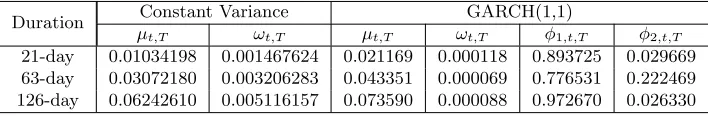
With respect to variance, two structures are assumed: (a) constant variance
over the whole span of the series, and (b) a GARCH(1,1) model for variance as
determined from real data. The GARCH(1,1) model is defined as [3]:
u
t,T,i=
µ
t,T+
ǫ
t,T,i,
ǫ
t,T,i∼
0, σ
t,T,i2σ
2t,T,i=
ω
t,T+
φ1
,t,Tǫ
2t,T,i−1+
φ2
,t,Tσ
2
t,T,i−1
(97)
The GARCH(1,1) model makes the individual return variances
σ
2t,T,i
of
log-returns fluctuate through time given that the unconditional historical variance
of the data still is a finite constant value.
The value
µ
t,Tfor simulations will be the mean as estimated from the S&P
500 data and will only change with respect to the contract duration and the
variance model of the case assumed. The statement
ǫ
t,T,i∼
0, σ
t,T,i2means
that the distribution will be generated from a standardized distribution that
will have zero mean. The standardized distribution depends on the value of
skewness and kurtosis. For the constant variance case,
φ1
,t,T=
φ2
,t,T= 0 is set.
Duration
Constant Variance
GARCH(1,1)
µ
t,Tω
t,Tµ
t,Tω
t,Tφ
1,t,Tφ
2,t,T21-day
0.01034198
0.001467624
0.021169
0.000118
0.893725
0.029669
63-day
0.03072180
0.003206283
0.043351
0.000069
0.776531
0.222469
[image:22.612.134.490.527.585.2]126-day
0.06242610
0.005116157
0.073590
0.000088
0.972670
0.026330
Table 1: Parameter Values for Variance Cases
Table 1 shows the values of the parameters for different cases. The estimates
of
µ
t,Tand
ω
t,Tfor the constant variance are the corresponding
Duration
S&P 500
Skewness Cases
Kurtosis Case
Skewness
Kurtosis
Negative
Positive
Leptokurtic
21-day
-1.034952
5.463981
-1.034952
1.034952
5.463981
63-day
-0.944574
4.170992
-0.944574
0.944574
4.170992
[image:23.612.152.463.145.203.2]126-day
-0.663999
3.705460
-0.663999
0.663999
3.705460
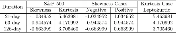
Table 2: Parameter Values for Skewness and Kurtosis Cases
About skewness, three cases are assumed: negative or skewed to the left, zero
or symmetric, and positive or skewed to the right. The value of skewness is
based on the S&P 500 data and would be different for every contract duration
considered. Table 2 shows the value of skewness per case and duration, based
on the skewness of the S&P 500 data. The formula used for the skewness of the
data is the following, based on equations (58) and (59):
ˆ
Skew
(u
t,T) =
ˆ
µ3
t(u
t,T)
h
ˆ
V ar
t(u
t,T)
i
3/2(98)
With respect to kurtosis, two cases are considered: the mesokurtic case,
where kurtosis is equal to 3, and the leptokurtic or heavy-tails case, where the
kurtosis is based on the S&P 500 data and returns based on contract duration.
Table 2 contains the values of kurtosis that will be used for the simulation
studies. The formula for kurtosis used to derive the values from data are the
following, based on equations (58) and (60):
ˆ
Kurt
(u
t,T) =
h
µ4
ˆ
t(u
t,T)
ˆ
V ar
t(u
t,T)
i
2(99)
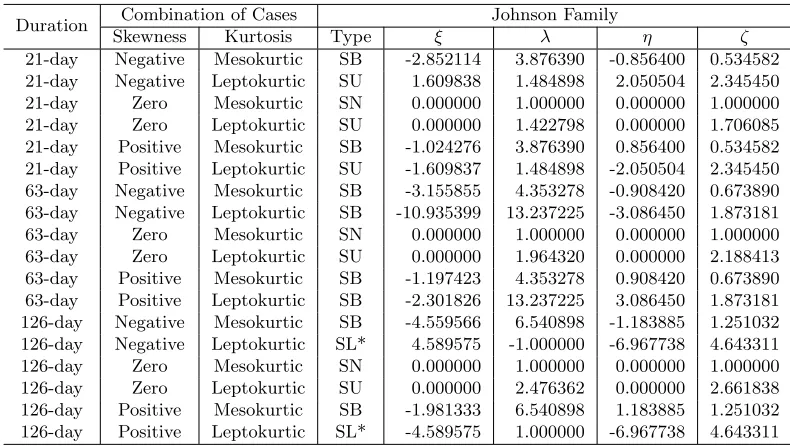
Since nonnormal features will be part of the cases of the simulations, when
nonzero skewness or nonnormal kurtosis is the case, then the Johnson family of
distributions [13] is used to generate the simulated returns data. The Johnson
family of distributions has the following cumulative distribution formula
F(x) :
F
(x) = Φ
η
+
ζ
×
g
x
−
ξ
λ
(100)
The function
g(
•
) is a function that determines the type of distribution used
for generating returns. If
g(z) =
z, then the Johnson distribution type is the
normal or Gaussian distribution, denoted as SN. If
g(z) = ln(z), then the
John-son distribution type is the lognormal distribution, marked as SL. The JohnJohn-son
SU or unbounded distribution type is generated by letting
g(z) = sinh
−1z, the
inverse hyperbolic sine function, and the bounded distribution or SB type is by
letting
g(z) = ln
1−zzThe parameters
ξ,
λ,
η, and
ζ
describe the location, scale, skewness, and
kur-tosis of the data, respectively; that is, changing the corresponding parameter
changes the specific feature of the distribution. They are not the exact values
of the mean, variance, skewness, nor kurtosis. However, the distribution
pa-rameters can be derived by moment-matching [11], of which estimated values of
the parameters and the type of distribution to be used are found through
solv-ing a system of nonlinear equations that matches the desired moment values to
the functions that describe the corresponding moments through the parameters.
Table 3 shows the different parameters and types of the Johnson family used
to generate each combination of cases for skewness and kurtosis. For each case,
it is assumed that the mean is zero and the variance is one since these can be
included over the simulated returns. An asterisk beside the SL indicates that
SB estimation would not converge, so the lognormal distribution was used to
approximate the nonnormal features.
Duration
Combination of Cases
Johnson Family
Skewness
Kurtosis
Type
ξ
λ
η
ζ
21-day
Negative
Mesokurtic
SB
-2.852114
3.876390
-0.856400
0.534582
21-day
Negative
Leptokurtic
SU
1.609838
1.484898
2.050504
2.345450
21-day
Zero
Mesokurtic
SN
0.000000
1.000000
0.000000
1.000000
21-day
Zero
Leptokurtic
SU
0.000000
1.422798
0.000000
1.706085
21-day
Positive
Mesokurtic
SB
-1.024276
3.876390
0.856400
0.534582
21-day
Positive
Leptokurtic
SU
-1.609837
1.484898
-2.050504
2.345450
63-day
Negative
Mesokurtic
SB
-3.155855
4.353278
-0.908420
0.673890
63-day
Negative
Leptokurtic
SB
-10.935399
13.237225
-3.086450
1.873181
63-day
Zero
Mesokurtic
SN
0.000000
1.000000
0.000000
1.000000
63-day
Zero
Leptokurtic
SU
0.000000
1.964320
0.000000
2.188413
63-day
Positive
Mesokurtic
SB
-1.197423
4.353278
0.908420
0.673890
63-day
Positive
Leptokurtic
SB
-2.301826
13.237225
3.086450
1.873181
126-day
Negative
Mesokurtic
SB
-4.559566
6.540898
-1.183885
1.251032
126-day
Negative
Leptokurtic
SL*
4.589575
-1.000000
-6.967738
4.643311
126-day
Zero
Mesokurtic
SN
0.000000
1.000000
0.000000
1.000000
126-day
Zero
Leptokurtic
SU
0.000000
2.476362
0.000000
2.661838
126-day
Positive
Mesokurtic
SB
-1.981333
6.540898
1.183885
1.251032
126-day
Positive
Leptokurtic
SL*
-4.589575
1.000000
-6.967738
4.643311
Table 3: Johnson Dsitribution Parameter Values and Types for Simulations
6
Results and Discussion
Table 4 contains the summary of simulation results considering the moneyness
and interest rate, ignoring other simulation scenari