Magnetic annihilation, null collapse and coronal heating

MAGNETIC ANNIHILATION, NULL COLLAPSE AND

CORONAL HEATING

Christopher Mellor

A Thesis Submitted for the Degree of PhD

at the

University of St Andrews

2004

Full metadata for this item is available in

St Andrews Research Repository

at:

http://research-repository.st-andrews.ac.uk/

Please use this identifier to cite or link to this item:

http://hdl.handle.net/10023/12946

L

Magnetic Annihilation, Null Collapse

and Coronal Heating

Christopher Mellor

Thesis submitted for the degree of Doctor of Philosophy

of the University of St Andrews

ProQuest Number: 10171057

All rights reserved

INFORMATION TO ALL USERS

The quality of this reproduction is dependent upon the quality of the copy submitted.

In the unlikely event that the author did not send a com plete manuscript and there are missing pages, these will be noted. Also, if material had to be removed,

a note will indicate the deletion.

uest

ProQuest 10171057

Published by ProQuest LLO (2017). Copyright of the Dissertation is held by the Author.

All rights reserved.

This work is protected against unauthorized copying under Title 17, United States C ode Microform Edition © ProQuest LLO.

ProQuest LLO.

789 East Eisenhower Parkway P.Q. Box 1346

Abstract

The problem of how the Sun’s corona is heated is of central importance to solar physics

research. In this thesis we model three main areas. The first, annihilation, is a feature

of non-ideal MHD and focusses on how magnetic field of opposite polarity meets at a null point and annihilates, after having been advected with plasma toward a stagnation point in the plasma flow. Generally, the null point of the field and the stagnation point of the flow are coincident at the origin, but in chapter 2 a simple extension is considered where an asymmetry in the boundary conditions of the field moves the null point away from the origin. Chapter 3 presents a model of reconnective annihilation in three dimensions. It represents flux being advected through the fan plane of a 3D null, and diffusing through a thin diffusion region before being annihilated at the spine line, and uses the method of matched asymptotic expansions to find the solution for small values of the resistivity.

The second area of the thesis covers null collapse. This is when the magnetic field

highly super-Alfvénic plasma flows.

The third area of this thesis involves numerically simulating a model of heating by

coronal tectonics (Priest et al, 2002). A simple magnetic field is created and the bound­

Declaration

1. I, Christopher Mellor, hereby certify that this thesis, which is approximately 35,000 words in length, has been written by me, that it is a record of work carried out by me and that it has not been submitted in any previous application for a higher degree.

date ... ... signature of candidate ...

2. I was admitted as a research student in October 2000 and as a candidate for the degree of PhD in October 2001; the higher study for which this is a record was carried out in the University of St Andrews between 2000 and 2003.

date . .14^. .1. R ...signature of candidate .. .w^... ...

3. I hereby certify that the candidate has fulfilled the conditions of the Resolution and Regulations appropriate to the degree of PhD in the University of St An­ drews and that the candidate is qualified to submit the thesis in application for that degree.

d a te kfV. r. ! .1 ___signature of supervisor...

4. In submitting this thesis to the University of St Andrews I understand that I am giving permission for it to be made available for use in accordance with the regulations of the University Library for the time being in force, subject to any copyright vested in the work not being affected thereby. I also understand that the title and abstract will be published and that a copy of the work may be made and supplied to any bona fide library or research worker.

Acknowledgements

Much praise and many thanks must be piled, nay heaped, upon

My parents, without whom I wouldn’t be here slaving away over a hot computer

My sister, Fiona

Cath

Eric Priest who took me on and gave me some of the years of his life

Klaus Galsgaard and Slava Titov for working and showing patience with me and giving me the ability to do the work

Dr Boothroyd and Dr Segar at Oriel College, who managed to steer me through all adversity towards my undergraduate degree

All my friends and the rest of my family who have helped me to keep my perspective

All the friendly people in the Solar Group, especially my office mates (David Boddie, Clare Foullon, Laura Carcedo and Robert Kevis)

I would like to acknowledge gratefully the financial support of PPARC. The numerical simulations were carried out using the JREI/SHEFC funded Compaq cluster and the PPARC/SRIF funded maths cluster in St Andrews.

Contents

Contents i

List of Figures v

1 Introduction 1

1.1 Overview of the Sun ... 2

1.2 Introduction to the Thesis... 4

1.2.1 The Validity of M H D ... 4

1.2.2 The MHD Equations... 5

1.2.3 The Structure of Two-Dimensional Null P o in ts ... 6

1.2.4 The Structure of Three-Dimensional Null Points ... 9

1.3 Null Point Collapse in Two D im ensions... 9

1.3.1 Equilibrium or Steady-State Structure of a N u ll... 9

1.3.2 Physical Cause of Collapse... 11

1.3.3 Linear Collapse... 13

1.3.4 Non-Linear C ollapse... 14

1.4 Null Point Collapse in Three Dimensions ... 17

1.4.1 Introduction... 17

1.4.2 Linear Collapse... 18

1.4.3 Non-Linear C ollapse... 21

1.5 Magnetic Annihilation in Two Dimensions... 23

1.5.1 Introduction... 23

1.5.2 Simple A nnihilation... 23

1.5.3 Stagnation-Point Flow M o d e l... 24

1.5.4 Time-Dependent Stagnation-Point F lo w ... 26

1.5.5 Reconnective Annihilation... 28

1.6.1 Introduction... 29

1.6.2 Fan Annihilation... 30

1.6.3 Spine Annihilation... 31

1.7 S um m ary... 31

2 Stagnation-Point Flow and Asymmetric Boundary Conditions 33 2.1 Introduction... 34

2.2 The M odel... 34

2.3 The Permissible Size of r ... 35

2.4 The Case With A Varying... 35

2.5 S um m ary... 36

3 Spine Reconnective Magnetic Annihilation 37 3.1 Form for new exact solutions... 38

3.1.1 Basic equations... 38

3.1.2 Proposed new solutions... 39

3.2 Solution for ai and ... 41

3.2.1 Outer solution ... 42

3.2.2 Inner solution... 43

3.2.3 M atching... 44

3.3 Solution for ao and ipQ ... 45

3.3.1 Outer solution ... 48

3.3.2 Inner solution... 48

3.3.3 M atching... 50

3.4 Properties of solutions ... 50

3.4.1 Fieldlines and stream lines... 50

3.4.2 The significance of 7 ... 52

3.5 Comparison of so lu tio n s... 55

3.5.1 The solutions of Craig & Fabling ... 55

3.5.2 Differences between the 2D and 3D c a se s... 55

3.5.3 The width of the current tube... 56

3.6 S um m ary... 57

4 Linear Collapse of Spatially Linear, Two-Dimensional Null Points 58 4.1 Introduction... 59

4.2.1 Model Equations... 59

4.2.2 Initial S ta te ... 61

4.2.3 Linearised Equations... 62

4.3 X -points... 65

4.3.1 Current-Free X -point... 65

4.3.2 The Symmetric C a s e ... 67

4.3.3 X-points with Current but No Flow ... 67

4.4 0-points... 70

4.4.1 Physical Cause of Collapse... 70

4.5 Effect of f lo w ... 72

4.6 S um m ary... 75

Collapse of Spatially Linear, Three-Dimensional Null Points 76 5.1 Introduction... 77

5.2 MHD and Model Equations... 77

5.2.1 Initial S ta te ... 77

5.2.2 Linearised Equations... 78

5.3 A Simple Physical Argument... 79

5.3.1 Collapse with a Spine C u rren t... 80

5.3.2 Collapse with a Fan C u n e n t... 81

5.4 Linear A nalysis... 83

5.4.1 jR ^ 1: the General C a se ... 83

5.4.2 R = l: the Axisymmetric Case ... 85

5.5 S um m ary... 88

Coronal Tectonics 89 6.1 Introduction... 90

6.2 Numerical Details... 90

6.3 The M odel... 93

6.3.1 The Initial Magnetic F ie ld ... 93

6.3.2 Driving on the Bottom Boundary ... 94

6.4 Results... 95

6.4.1 Current Scaling... 95

6.4.2 Slower d riv in g ... 97

6.4.3 Reconnection... 98

6.5 S um m ary... 105

7 Conclusions and Further Work 106 7.1 Magnetic A nnihilation... 107

7.1.1 Stagnation-Point Flow and Asymmetric Boundary C onditions... 107

7.1.2 Spine Reconnective Annihilation... 107

7.2 Null C ollapse... 108

7.2.1 Collapse in 2 D ... 108

7.2.2 Collapse in 3 D ... 108

7.3 Coronal Tectonics... 109

8 Bibliography 111

List of Figures

1.1 A schematic diagram of the Sun, showing the core, the radiative zone and the convective zone... 2 1.2 Three-dimensional fieldline plot showing the magnetic skeleton due to three un­

balanced sources (black stars). The red dome is the separatrix surface forming the fan of the null point (black spot) on the left and the thicker red line is its spine. The blue dome and thicker line are the equivalent structures for the other null point. The dotted purple line is the separator which joins the two null points. This is also the curve where the two separatrix domes intersect... 3

1.3 Magnetic field lines for the four types of two-dimensional null point. {Top Left)

A potential X-point {j = 0). {Top Right) A non-potential X-point (|j| < jc). {Bottom Left) A one-dimensional current sheet {\j\ = jc). {Bottom Right) An O-point (|j| > jc .)... 8 1.4 A potential three-dimensional null point. The spine is the blue vetical line and the

fan plane is the light blue plane. Fieldlines lying in the fan plane are red and a selection of other fieldlines are black... 10 1.5 The magnetic field lines near an X-type null point, with distance measured in

dimensionless units x /l and y /I. The field line spacing depends on the strength of the field. {Left) In equilibrium with no current. {Right) Away from equilibrium (e = 0.96) with the resultant force on the x- and y-axes indicated by the thick arrows. It can be seen that this force will carry on the collapse of the X-point. . . 13

1.6 Evolution of field lines in the fundamental mode for linear X-point collapse in­

cluding magnetic diffusion and anchoring the footpoints to the circular boundary. The number above each plot is the number of cycles of oscillation that have passed. After three cycles the system is close to its equilibrium neutral point configuration.

1.7 {Left) The dimensionless flux function (a) as a function of dimensionless time r and different values of (5o (<^o — 0.01, the red line; (5q = 0.03162, the green line; <5o — 0.1, the blue line) for the non-linear collapse of a potential X-point. {Right)

The dimensionless velocity (7) as a function of r. The functions become singular

in a finite time, thus collapsing the null... 17 1.8 The linear collapse of a potential null due to the growth of a spine current along

the z-axis. The field lines within the fan plane collapse over time (Parnell et al,

1997)... 20 1.9 The lineal' collapse of a potential null due to the growth of a fan current along the

æ-axis. The angle between the spine and fan decreases over time. (Parnell et al,

1997) 20

1.10 The non-linear collapse of a potential null point due to growth of the spine current, causing the spine to flatten out. (Bulanov and Sakai, 1 9 9 7 )... 22 1.11 The non-linear collapse of a potential null point due to the growth of the fan cur­

rent, causing the spine to collapse into the fan plane. (Bulanov and Sakai, 1997) . 22 1.12 The ohmic decay of a simple current sheet with a one-dimensional magnetic field

B {x,t)y. The initial field profile is the black line, the blue line represents the profile at t = 1/4, the green line at t — 7/4 and the red line at t — 4 9 /4 ... 24 1.13 The stagnation-point flow model for magnetic annihilation. {Left) The velocity

stream lines (thick) and the magnetic field lines (thin). The shaded region denotes the diffusion region. {Right) A plot of the field strength {B) as a function of distance x... 25 1.14 Time-dependent magnetic annihilation. {Top) The initial profile B(y) = y /(l +

y^'®). (a) The development of the field for times t = 0,1.2,2.4...7.2, and (b) the resulting magnetic properties. {Bottom) The initial profile B{y) = y /(l + y^'^). (a) The development of the field for times t = 0 ,1.4,2.8. ..7, and (b) the resulting magnetic properties. (Anderson and Priest, 1 9 9 3 )... 27 1.15 The streamlines (dashed) and the field lines (solid) for two-dimensional reconnec­

tive annihilation. The diffusion region is shaded grey and the arrows indicate the direction of the field and flow, both inflowing on the boundary. (Priest et al, 2000) 29 1.16 The advection of field lines across the spine of a null point in a model of fan

reconnective annihilation. The same plasma element is followed and one can see that a field line frozen into the plasma crosses the spine and diffuses in the fan. (Craig a/, 1995)... 31

3.1 The variation of A and A with the parameter 7... 43 3.2 (Top) ai as a function of s for 77 = 0.01, Brq = 2, A = 2 and k = 500. (Bottom)

•01 as a function of s for ij = 0.01, Brc = 2, X ~ 2 and k = 500... 46

3.3 (Top) d^ai/ds^ as a function of 5 showing the boundary-layer nature of the solu­ tion. The solid curve is the full numerical solution, the dashed curve is the outer solution and the dotted curve the inner solution. (Bottom) d^ai/ds^ as a function of s for the values 77 = 0.001,0.003,0.01 and 0.03 that increase from left to right as the width of the boundary layer increases. All other parameters are as in Figure

3.2 47

3.4 (Top) ao as a function of 5. The parameters are the same as previously, with Vze = 5 and Bze = —1.83 also. (Middle) 0o as a function of s. (Bottom) f^aojds^

as a function of s with 77 = 0.01 displaying the boundary-layer nature of the solution. 51 3.5 (Top left) Fieldlines for the case 7 = 0.665 and c = 0. (Top right) Streamlines for

the case 7 = 0.665 and c = 0. (Bottom left) Fieldlines for the case 7 = 0.665 and c = 5. (Bottom right) Streamlines for the case 7 = 0.665 and c — 5... 52 3.6 (Top left) Fieldlines for the case 7 = 1 and c = 0. (Top right) Streamlines for the

case 7 = 1 and c = 0. (Bottom left) Fieldlines for the case 7 = 1 and c — 5. (Bottom right) Streamlines for the case 7 = 1 and c = 5... 53 3.7 (Top left) Fieldlines for the case 7 = 1.420 and c == 0. (Right) Streamlines for the case 7 = 1.420 and c = 0. (Bottom left) Fieldlines for the case 7 = 1.420 and c = 5. (Bottom right) Streamlines for the case 7 = 1.420 and c = 5 ... 53 3.8 Stream surfaces viewed from above, showing that, as |c| increases, one of the

cylinders grows in size and wraps around the other one. This example is for 7 =

1.420 and c = 0, 6, 12 and 18 from top left to bottom right... 54 3.9 The variation of the current tube width (I) with 7 and \BRe/vRe\. Starting from

0.25 on the bottom curve, 7 increases in steps of 0.25 up to a value of 2 on the top curve... 57

4.1 A plot of the magnetic field lines of an X-point with the initial state ckq = 1 (dotted curves) and the perturbed state having a = 1.2 (solid curves). The arrows show

the direction and relative magnitude of the additional force acting on the plasma. 69

4.2 The growth rates (A) of the pressure perturbations P u (left) and P22 (right) as

functions of the dimensionless current (Jo)... 70 4.3 A plot of the magnetic field lines of an O-point with ckq = 1 (dotted ellipses) and

the perturbed field witli a = 1.2 (solid ellipses). The arrows indicate the direction and relative strength of the additional force acting on the plasma... 72

4.4 Plots of the regions in Jq-Ma parameter space where different perturbations have

growing solutions. The sets of three letters indicate the stability to collapse of the pressure elements in that particular region. Thus, for instance, “uss” would indicate that P u in unstable to collapse, whereas P12 and P22 are both stable to collapse. The top figure shows one completely stable region. The bottom figure shows the region for 0 < Jo < 1 and 0 < Ma < 1, i.e., an X-point... 73

5.1 Introducing a Spine Current. (Left) The collapse of the null in the xy plane in the case P = 0.5. (Right) The collapse of the null in the xy plane in the case R — 1.

The thin, dotted lines are the unperturbed fieldlines, whereas the thick, solid lines are the perturbed fieldlines (e = 0.3) and the arrows show the relative strength and direction of the induced Lorentz force which is seen to increase the perturbation and so collapse the null... 80

5.2 Introducing a Fan Current. (Left) The collapse of the null in the yz-plane in the

case R — 0.5. (Right) The collapse of the null in the yz-plane in the case R = l.

The lines and airows are as in Fig 1 and e = 0.5. For all values of R, the Lorentz force is in a direction such as to increase the perturbation and collapse the null. . 82 5.3 as a function of vu). For all positive values of vu, X? is also positive and so

there is a positive growth rate which causes the null point to collapse... 88

6.1 Priest et al (2002) suggest that a TRACE loop is made up from many smaller loops

which separately embed themselves into the photosphere... 90 6.2 Model coronal loops produced by discrete magnetic sources (starred) located in

the planes z; = ±L. Null points (dots) and separatrix surfaces (dashed) are also indicated... 91 6.3 A typical cell demonstrating the staggering of the variables... 93

6.4 The initial axial magnetic field strength on the top and bottom boundaries . . . . 94

6.5 The driving velocity on the bottom boundary. Red is the inputted function and black is the smoothed function in the case of 129^... 95 6.6 A plot of \jmax\ against grid resolution. The squares are the experimental results

and the line is the line of best fit... 96 6.7 A plot of jmax in the plane x ~ 0.5 for the 129^ iTins with a driven speed of

-0.03 (solid line) and -0.01 (dashed line). The current jumps in value initially as the information propagates through this plane. As the footpoint displacement increases, the middle plane is being affected from above and below, so the current grows more smoothly. The cunent in both cases is growing at approximately the same rate for a given displacement... 97

6.8 Plots of the cunent isosurface |j| = 2 for the two different driving speeds at a footpoint displacement of 0.47. The quicker speed —0.03 is shown on the left and the slower speed —0.01 on the right... 98 6.9 Contours of |jl = 3.6 showing that the current sheet is thin. (Left) The whole of

the æ = 0.5 plane (Right) A close-up of the upper contour, showing it to be fewer than three grid points wide... 99 6.10 A representation of the Petschek reconnection model for comparison with figures

6.11 and 6. 1 2 ... 99 6.11 (Top Left) Current contours with velocity streaklines in the æ = 0.5 plane at i =

Ib.YtA- (Top Right) Vorticity contours with velocity streaklines in the x — 0.5 plane at t = 15.7^^* (Bottom Left) A close-up of the bottom portion of top left to show better detail. (Bottom Right) A close-up of the bottom portion of top right to show better detail. The shocks are not very well defined at this time, but can just about be seen... 101 6.12 (Top Left) Cunent contours with velocity streaklines in the x = 0.5 plane at t —

32.1iy4. (Top Right) Vorticity contours with velocity streaklines in the æ == 0.5 plane att = 32.It a- (Bottom Left) A close-up of the bottom portion of top left to

show better detail. (Bottom Right) A close-up of the bottom portion of top right to show better detail. The shocks are much better defined at this time... 102 6.13 Plots of |j| = 3 (green), |j -B |/(|j||B |) = 1 (red) and a selection of magnetic field

lines (blue) for t = 13.8, 30.7, 35.4 and 42.1tyi from top left to bottom right. During the time between the last two plots, one of the fieldlines appears to have reconnected through the current sheet... 103 6.14 A plot showing the same as figure 6.13, but viewed from above the z = 1 plane and

at i = 37.2ÎA’ The fieldlines’ starting points are in a line through the current sheet and the one that starts immediately above this sheet appears to have reconnected through it... 104 6.15 (Left) The Joule dissipation throughout the numerical box during the course of

the experiment. Energy is being converted into heat from an early time. (Right)

The Poynting flux through the bottom boundary (solid line) and the kinetic energy (dashed line). These increase and decrease in a pattern that follows the reflection of Alfvén waves from the top and bottom boundaries... 104

Chapter 1

Introduction

<sm»

1_{<2:*!»x**:*xw} mvm

SCHOOL

THE GIFTED

1.1 Overview of the Sun

1.1 Overview of the Sun

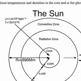
Containing over 99% of the total mass in the solar system, the Sun is our nearest star and the source of life on Earth. It is no wonder that, as such, it is an obvious focus of scientific interest. The Sun is a huge, searing hot ball of ionised plasma, powered by nuclear fusion. Fig 1.1 shows a simple section through the Sun, showing the core, radiative zone, convective zone and some information about temperatures and densities in the core and at the photospheric surface.

The Sun

p=l.6x105 kgm-3

T=15x10®K _{Convective Zone}

Radiative Zone

Core

R= 696Mm

0.25R

0.45R

0.3R

Photosphere T=6000K

p=10“^kgm"3

Figure 1.1: A schematic diagram of the Sun, showing the core, the radiative zone and the convec­ tive zone.

The atmosphere of the Sun is divided into three tiers. The photosphere, chromosphere and of most interest for the purposes of this thesis, the corona. The corona is the outermost part of the Sun and stretches from 4000km above the surface, right out past the Earth and other planets as the solar wind. It is extremely tenuous {p = 10“ ^^kgm“ ^) and very hot (T > lO^K). One of the

biggest questions in the study of the corona is why is it so much hotter than the photosphere and

chromosphere? It is widely believed that the magnetic field in the corona is responsible.

1.1 Overview of the Sun

charges in this solar dynamo give rise to a magnetic field which is transported to the surface of the Sun by magnetic buoyancy in the convective zone. Once the field has emerged into the corona, the forces it exerts are much stronger than those due to the coronal plasma. This means that it is the magnetic field rather than the plasma that acts as the driving force for coronal phenomena.

Among the most important magnetic processes is magnetic reconnection. This happens when a region of strong current allows magnetic field lines to break and join to other field lines. This change of connectivity releases energy which was previously stored in the magnetic field and is thought to be one of the reasons why the corona is so hot. Some of the regions which may be important to the occurrence of reconnection are included in the topological skeleton of the magnetic field. The skeleton of a magnetic field is made up of the null points of the field, the spines and fans (explained later) associated with these nulls, and the separators (field lines joining two nulls) and séparatrices (the intersections of fans which mark the boundaries of regions of different magnetic connectivity). Figure 1.2 shows an example of a magnetic skeleton due to three unbalanced photospheric magnetic sources.

Separator

Null Poi

Sourc

Figure 1.2; Three-dimensional fieldline plot showing the magnetic skeleton due to three unbal­ anced sources (black stars). The red dome is the separatrix surface forming the fan of the null point (black spot) on the left and the thicker red line is its spine. The blue dome and thicker line are the equivalent structures for the other null point. The dotted purple line is the separator which joins the two null points. This is also the curve where the two separatrix domes intersect.

1.2 Introduction to the Thesis

where current sheets are seen to build up at quasi-separatrix layers.

1.2 Introduction to the Thesis

The universe consists mainly of ionised gas, or plasma, which often forms highly dynamic and complex systems. When a plasma interacts with a magnetic field, such as in the corona of a star, it may be structured, heated and also accelerated by the field. The two are coupled to each other in a subtle non-lineai* manner. In this environment the magnetohydrodynamic (MHD) equations are often appropriate for modelling a wide range of processes.

A very important process that occurs in a magnetised plasma is magnetic reconnection at a null point. This causes a change in magnetic topology to take place due to field lines changing their connectivity. The process often releases a great deal of energy that was previously stored in the field. It is thought to be at least partially responsible for the heating of the solar corona and for many other phenomena in laboratory, space, solar and astrophysical plasmas. Reconnection can occur when a strong current causes the field lines to diffuse through the plasma and become connected to different field lines. In three dimensions, reconnection can occur either at null points (e.g., Priest and Titov, 1996; Galsgaard and Nordlund, 1997b) or in the absence of null points (e.g. Schindler et al, 1988; Priest and Forbes, 1989; Priest and Demoulin, 1995; Hornig and Rast atter,

1998). A detailed account of all these aspects can be found in a recent monograph (Priest and Forbes, 2000).

Null points are locations where the magnetic field vanishes. When one of these points col­ lapses, a strong current sheet is formed around the null. The current sheet may be the catalyst for an increase in resistivity in the plasma which can trigger fast reconnection. This introduction con­ centrates on existing exact solutions for the collapse of null points and the resulting annihilation of magnetic field.

1.2.1 The Validity of MHD

There are several approximations under which MHD is valid. These are discussed further in Priest (1982), Goedbloed (1983) and Biskamp (1993). They can be summarised briefly as follows.

1. The MHD equations are single fluid equations.

2. The length-scale under consideration is much laiger than the Debye length,

1.2 Introduction to the Thesis

where eo is the permeability of free space, is the Boltzman constant, T is the temperature

of the plasma, e is the ion charge and Ue is the ion number density.

3. The length-scale under consideration is also much larger than r = {2mkBT)^/‘^/eB, the

ion-gyro radius, where m is the ion mass and B is the field strength across the electric field. 4. All velocities under consideration are much less than the speed of light, such that the dis­

placement current, {dE/dt)/c^, in Ampére’s law can be neglected.

5. The factor of 2 in the ideal gas law is for a hydrogen plasma. This is a good approximation in the solar corona.

1.2.2 The MHD Equations

The MHD equations for v, B, p, p that we shall employ are equations 1.1-1.9, namely, the induc­

tion equation

^ = V x ( v x B ) + )7V^B, (1.1)

Ohm’s Law

j — (j(E -}- V X B), (1.2)

the equation of motion

Dy _{= - V p - f j X B-f/O g-j-F, (1.3)}

the equation of mass continuity

^ + V -(pv) = 0, (1.4)

the ideal gas law

P = 2pRT, (1.5)

and an energy equation such as

(1.6) ■y — 1 Dt \p'^ J (T

with the initial constraint

1.2 Introduction to the Thesis

where B is the magnetic field, v is the plasma velocity, p is the plasma density, j is the current density, p is the thermal plasma pressure, g is the acceleration due to gravity, F is the force due to other effects, such as viscosity and 7 is the ratio of specific heats. The permeability is pq and the diffusivity of the plasma is 77 = l / ( / U o c r ) where <7is the conductivity (all assumed to be constant).

The primary variables, v, B and p can be determined from Equations 1.1-1.5. The secondary variables E (the electric field) and j then result from Ampere’s and Faraday’s laws, namely,

j = — V x B , (1.8)

Mo

V x E = - ^ . (1.9)

1.2.3 The Structure of Two-Dimensional Null Points

Null (or neutral) points occur where the local magnetic field vanishes. In the linear approximation, the magnetic field B near a null point can be represented as

B = M - r , (1.10)

where M is a matrix with elements M{j = dB i/dxj and r is the position vector.

In two dimensions (x,y), the most general form for M is

M =

where p and q are associated with the potential part of the field and j/po is the current in the z-direction. The associated flux function {A) satisfies

B x - g ÿ , B y - - - ^ ,

and has the form

A = \ { { q - j)Y ^ - i q + j)X ^) + pXY. (1.11)

By rotating the axes we may eliminate the X Y term and reduce this to

1.2 Introduction to the Thesis

where

Jc = (1 13)

is a critical current.

Four different cases arise, as follows

i. 3 = 0.

The flux function then becomes

A = jc{y^

-which implies that the field lines are rectangular hyperbolae. The séparatrices through the null in this case intersect at right angles. It is referred to as a potential null, since there is no current associated with the field.

ii- lil <

Jc-The flux function here gives hyperbolic field lines with séparatrices that intersect at an angle of

This is a non-potential X-point. As j -> 0, the field lines tend to rectangular hyperbolae as in the first case.

iii-

\j\=3c-The flux function now depends only on if jc = j and only if jc = - j . The config­

uration has antiparallel field lines with a null line along the y or æ-axis, respectively, and represents a one-dimensional current sheet.

iv. lit >

3c-The flux function produces concentric ellipses as field lines so the configuration is called an O-point. The ratio of the semi-major and semi-minor axes of the ellipses is

j

+

j - jc )

As jc /j — 0, these become circular.

1,2 Introduction to the Thesis

0.5 0.5

—0.5 0.5

--1

1 -0.5 0.5

-0,5 0.5

1

0.5 0.5

-0.5 -0.5

- 1

-0.5 1 -0.5 0.5

-0.5

Figure 1,3: Magnetic field lines for the four types of two-dimensional null point. {Top Left) A potential X-point (j = 0). {Top Right) A non-potential X-point (|y| < jc). {Bottom Left) A

1.3 Null Point Collapse in Two Dimensions

1.2.4 The Structure of Three-Dimensional Null Points

The simplest form that M (Equation 1.10) can take in three dimensions is

M =

1 \{Q - J\\) 0

1(Q + J||) R 0

0 </jL —{R + 1 ) _

(1.14)

where Jn+4i? and the current is

The potential part of the field is determined by the parameters R and Q, J|| is the current parallel to the z-axis, which is known as the spine, and Jj_ is the current perpendicular to the spine. The effects of varying the various parameters and an in-depth treatment of the structure of these nulls has been given by Parnell et al (1996). In general, the skeleton of a three-dimensional null consists of a spine curve and a fan plane. The spine is a field line through the null following the eigenvector of the matrix M that is associated with the eigenvalue which has a different sign from the other two eigenvalues. The fan is a surface through the null which is defined by the eigenvectors of M associated with the remaining eigenvalues (Priest and Titov, 1996). A potential null has spine and fan perpendicular to each other. Increasing Jx increases the angle between spine and fan whereas varying Jy changes the structure of the field lines in the fan. Figure 1.4 shows a simple potential three-dimensional null point, highlighting the location of the spine and the fan.

1.3 Null Point Collapse in Two Dimensions

1.3.1 Equilibrium or Steady-State Structure of a Null

In an ideal steady state, the magnetic field, plasma velocity, plasma pressure and density must satisfy the time-independent MHD equations

V X (v X B) = 0, (1.15)

p(v • V)v = -V p -f j X B, (1.16)

1.3 Null Point Collapse in Two Dimensions 10

Figure 1.4: A potential three-dimensional null point. The spine is the blue vetical line and the fan plane is the light blue plane. Fieldlines lying in the fan plane are red and a selection of other fieldlines are black.

P

— = constant (in the compressible case),

p = constant (in the incompressible case). (1.18)

In two dimensions, consider first the simplest null point, a potential X-point, where the séparatrices are at right angles and there is no current. The equations are satisfied identically when v = 0 and Vp = 0, so that there is no plasma flow and the pressure is uniform throughout the space which we are considering close to the null.

If we next consider a circular O-point, whose field components are BQ{—y,x)/l, the steady-

state equations are satisfied with a balance between just the magnetic and centrifugal forces when

the plasma flow is directed along the magnetic field and has magnitude V2vA{—y, x)/I, where va

is the Alfvén speed, Bo/{popŸ^^. This represents a super-Alfvénic flow parallel to the field and so is unlikely to occur easily in practice. However, if a slower flow v = vo{—y ,x )/l is present, then a pressure gradient of

Mo (1.19)

can balance the centrifugal and magnetic forces. For an X-point with current, or an elliptical O- point, neither a plasma flow nor a pressure gradient on its own can support the magnetic field, so

1.3 Null Point Collapse in Two Dimensions________________________________________ H

and vo{ay, x)/l, respectively, then the supporting pressure gradient is

1 f {-appQV^ + B^{a - l))x \

Vp = _pol^

I -{app,Qvl + aB l{a - l))y

With these spatially linear forms for the magnetic field and velocity, the form that is adopted for the plasma pressure is different for a compressible and an incompressible plasma regime. In the compressible case, the pressure (po + Pi) and density (po + pi) are assumed to be functions of time alone and independent of space, such that the compressible part of 1.18 is satisfied. After non-dimensionalising and linearising, the equations of motion and mass continuity then become

p o ^ ^ + Po(vo • V )vi + pi(vo • V)vo + po(vi • V)vo

= (V X B i) X Bo 4- (V X Bq) X B i, (1.20)

^ + « V - v i = 0, (1.21)

where a subscript 0 denotes the initial, steady state and a subscript 1 indicates the small perturba­ tion. In order to satisfy (1.20), the densities (po, pi) and pressures (po, pi) are spatially uniform, so there is no spatial pressure gradient.

In the incompressible case, po is constant and pi vanishes. After non-dimensionalising and linearising, the equations of motion and continuity instead become

+ (vo ' V )vi + (vi • V)vo = — Vpi (V X Bo) x B i + (V x B i) x Bo, (1.22)

V - v i = 0. (1.23)

The constant density (po) has been scaled out, but this time 1.22 can be satisfied by assuming the perturbed pressure (pi) is a quadratic function of x and y since there is no (adiabatic) energy equation restiicting its form.

1.3.2 Physical Cause of Collapse

1.3 Null Point Collapse in Two Dimensions 12

Consider the initial magnetic field with components

Bo. = Boy = ^ x , (1.24)

where Bq and I scale the magnetic field and distance, respectively. The field has rectangular

hyperbolae for field lines, described by

~ constant, (1.25)

as shown in Figure 1.5. The current (jo — (V x Bo)/mo) of this field vanishes, so that the force (jo X Bo) exerted by the field on the plasma is also zero, and tlie field is in equilibrium with itself.

Now consider a perturbation to the field of

B\y = e-j-x, (1.26)

so that the perturbed field (B = Bo + B i) is now

Bx = By — {1 + e ) - ~ x . (T27)

and the field lines are

- (1 + e)x‘^ — constant, (1.28)

with the séparatrices now no longer perpendicular to each other, but described by

2/ = ± ( l + e)^/^a;, (1.29)

much like the closing of a pair of scissors. The field is no longer current-free and possesses a current,

ji -= — T&, _Pol (1.30)

which means that the linear force exerted by the field is now

j l x B = ^ ( - r c x + ÿÿ}. (1.31)

The directions of this force are such as to carry on closing the X-point until it collapses completely, also shown in Figure 1.5. As the field lines close up in this way and e increases, so the ohmic

1.3 Null Point Collapse in Two Dimensions 13

/

-2 -2

-3: -3

-3 -2 4 -3 -2

Figure 1.5: The magnetic field lines near an X-type null point, with distance measured in dimen- sionless units xjl and yjl. The field line spacing depends on the strength of the field. {Left) In equilibrium with no current. {Right) Away from equilibrium (e = 0.96) with the resultant force on the X - and ^-axes indicated by the thick arrows. It can be seen that this force will carry on the

collapse of the X-point.

1.3.3 Linear Collapse

Linear analyses of the collapse problem have been carried out using perturbation techniques by

many people during the 1990s (e.g., Bulanov et al, 1990; Craig and McClymont, 1991; Hassam,

1992; Fontenla, 1993 and Titov and Priest, 1993). These treatments demonstrate that collapse occurs for a wide variety of initial and boundary conditions. It must be stressed that when one talks about linear collapse (as they do in the literature on the subject), what is really being talked about is a linear instability. In principle, when the linear perturbation grows large enough for non-linear terms to become important, these may possibly halt the collapse. The linear results are obtained by linearising the MHD equations and using an initial flux function describing a potential X-point (Ao = BqI{x^ — y^)) where x = x/l and ÿ = y /I. Setting the pressure to zero leads to a

third-order, linear differential equation for the linear perturbation (Ai), namely.

= (^2 -H -f

d î (1.32)

The dimensionless time is ( = tvAo/l and the dimensionless diffusivity is fj = t]/{vaoI), where VAo is the Alfvén speed, 5o/(p/xo)^^^- There are several ways to solve this equation, and here we follow Craig and McClymont (1991).

1.3 Null Point Collapse in Two Dimensions________________________________________ 14

polar coordinates, the equation for /( r ) becomes,

0-33)

where f = df /dr. The perturbation (Ai) is set equal to a constant on the boundary, r = 1, which freezes the field lines to the boundary.

Very close to the origin, equation (1.32) reduces to the diffusion equation

^ = (1.34)

giving a solution

Aim = exp(im(/>+ At),

in terms of the Bessel function ( J^).

Away from the origin, in the advection region, Equation (1.32) reduces to the wave equation,

Al _{= r V A i .} Ov72 _(1.35)

The speed of the wave, and thus the information travelling in from the boundary, varies as the distance (r) from the origin. The only mode, however, which allows topological reconnection at the origin is the m = 0 mode, due to the Bessel function form of the current near the origin.

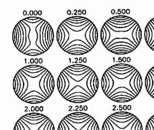
Figure 1.6 shows the evolution of the field lines in the fundamental mode (m = 0 with no nodes in the radial direction). The field lines can be seen to be oscillating to and from the null. At the end of the three cycles shown, the system is very close to its equilibrium null point con­ figuration with magnetic diffusion having been responsible for the dissipation of the energy in the system.

1.3.4 Non-Linear Collapse

Whilst Dungey (1953) considered the linear evolution of an initially potential X-type null point, Imshennik and Syrovatsky (1967) extended this by studying the non-linear evolution of an X- point with a compressible flow. They solved the equations

d dA ^ _

dva^ __ dp 1 dA 2 A p - ~ —

1.3 Null Point Collapse in Two Dimensions 15

0.000 0,250

0.500

0,750

1.750

1.250

1.000

2.750

2,500

2.250

Figure 1.6: Evolution of field lines in the fundamental mode for linear X-point collapse including magnetic diffusion and anchoring the footpoints to the circular boundary. The number above each plot is the number of cycles of oscillation that have passed. After three cycles the system is close to its equilibrium neutral point configuration. (Craig and McClymont, 1991)

dVr dp 1 d A,

dt dy ^0 dy

dp

dt -t- pV.v = 0. (1.36)

A is the magnetic flux function and d/dt is the advective time-derivative. The pressure (p) is assumed to be a function of the density only, with a polytropic equation of state so that p — p{t), p = p{t) and Vp = 0. Their initial conditions were

p(æ,p,0) = po, A(æ,p,0) = - p^),

U y

%/, 0) — 0) — ,

where po, Aq, 17, V are constant. Non-dimensionalising and introducing the new variables (1.37)

t

^= 7o ' 5 = 7 ’

X

1.3 Null Point Collapse in Two Dimensions________________________________________ ^

where vq— Ao/(Z(poPo)^^^) and to = 1/vq, the Equations (1.36) may be written,

dx dr ' dÿ dr ’

dr dx dr dy

^ + p V - v = 0. _dr (1.39)

The initial conditions become

p(x,ÿ,Ü) = l, A{x,v,0) = x^ -ÿ'^, %{x,v,0) = 'loS, Vy[x,y,0) = âov,

where

^ A ^

70 = — , oq = — •

Vo Vo

The system has a solution of the form

À{x,ÿ,r) = a{r)x‘^ - P{r)y‘^, p{x,y,r) = p{r), Va,(æ, p, r) = 7(r)æ,

Vy{^,ÿ,r) = ô{r)ÿ,

with the unknown functions of r determined by the following non-linear equations,

à + 2cK7 = 0, ^ -f 2^^ = 0, p(7 -t-7^) = a(^ — a), p p { ' y - h 5) = 0,

where / = df/d r and the initial conditions are a (0) = 1, /3(0) = 1, 7(0) = 70, 5(0) = 5q and

p(0) = 1

Figure 1.7 shows how a and 7 vary with r, for the initial conditions 70 = 0 and different values of 5q. It can be seen that the solution for these functions blows up after a finite time, which implies that the X-point collapses.

The solutions were shown to become singular at a time tq with an asymptotic behaviour as

T —)■ To given by

a o c a i , /5 oc (ro - r ) “ ^/^, 7 oc 7 1,

5 o c ( r o - r ) ~ \ p oc (tq - r)~^/^. (1.40)

ai, 7i and tq depend on the initial conditions and are found by solving the system of equations

1.4 Null Point Collapse in Three Dimensions 17

5 _0.5

2.5

i

4

3

-2

a

2

- 3 1

0 _{0.5 1 1.5 2 2.5 3}

-5

Figure 1,7; (Left) The dimensionless flux function (a) as a function of dimensionless time r and different values of So (Sq = 0.01, the red line; Jq = 0.03162, the green line; Sq = 0.1, the blue line) for the non-linear collapse of a potential X-point. (Right) The dimensionless velocity (7) as a function of r. The functions become singular in a finite time, thus collapsing the null.

Other investigations into the collapse of an X-point have been carried out by Chapman and Kendall (1963) and Forbes and Speiser (1979). Later, Neukirch (1995), Neukirch and Priest (2000) and Neukirch and Cheung (2001) found special solutions to the time-dependent MHD equations for an ideal isothermal plasma in which the plasma elements experience no accelera­ tion, or alternatively an acceleration caused by a potential force.

The importance of the open boundary conditions was emphasised by Klapper (1998) who showed that in ideal, two-dimensional, incompressible MHD, a singularity cannot occur in a finite time unless driven by some non-local singularity in the pressure. This is consistent with the original physical argument of Dungey (1953), which needed open boundary conditions to allow energy to propagate into the system from outside.

1.4 Null Point Collapse in Three Dimensions

1.4.1 Introduction

1.4 Null Point Collapse in Three Dimensions 18

of the j X B force can only be zero when the null point is current-free (or potential).

Other three-dimensional nulls can be supported by a combination of the plasma flow and a pressure gradient. Such flows and pressure gradients were found by Titov and Hornig (2000) for the case of incompressible plasma flow. They used the linear three-dimensional magnetic field given in Equation 1.14 for their field (B) and solved the matrix equations

y2 _ yT2 ^T2 _(1.41)

ir(V) = 0, tr{B) = 0, (1.42)

VB = BV, (1.43)

r = B'^~ B'^B - (1.44)

to find the plasma velocity (V) and the pressure gradient matrices. They again discovered that a flow parallel to the field at the Alfvén speed could support the field. However for a null point with spiral field lines in its fan (| J|j| > ((i? — 1)^ -f there are other, non-trivial flows that can sustain the field.

1.4.2 Linear Collapse

As was mentioned in the introduction, by making certain rotations and scalings, the simplest form in which to express the magnetic field close to a null point is B = M r, where r is the position vector and M is the 3 x 3 matrix

M =

1 | ( Q - J j | ) 0

\{Q J\\) R

0

0 J_L

(Parnell et al, 1996) where R and Q represent the potential parts of the field, and Jy and J_l are the current parallel and perpendicular to the %-axis respectively. When R > —1 the eigenvector along the z-axis is always pointing toward the null, and the other two eigenvectors are always pointing away from the null. The z-axis therefore represents the spine and the other two eigenvectors lie in the plane of the fan (Priest and Titov, 1996).

Parnell et al (1997) considered three-dimensional potential nulls

Bq = Ry, —{R + 1)^],

1.4 Null Point Collapse in Three Dimensions 19

current into the system, they solved the linearised, compressible MHD equations, including

= V X (vi X Bo),

= — ( V X B i ) X B q ,

Ut flQ

where B = Bq 4- eBi, and v = evi with e <C 1. The resulting density perturbation follows from the continuity equation. They found that the solutions grow exponentially whatever the form of current introduced by the perturbation. These growing solutions indicate that the null point will tend to collapse provided that the footpoints of the field lines are free to move on some boundary.

When a current is introduced perpendicular to the spine, the solutions are of the form

/

\

B i = eBoJ__{1{2R + 1)}L6^^

VI = evAJ±e:

V

/

( B + l ) z

R y

0 \

(RT l)z

\ Ry /

l(2R + l)

where va = Ro/ipoMo)^^^ and the growth rate cu = (2R + 1)va/L

When a current is instead introduced parallel to the spine, the solutions are of the form

B i = _{l ( R - l )}

VI = €VAJ\\ë

w, /

\ 0 y

l \ R - l \

where va — Bq/ a n d the growth rate oj = \R — 1\va

1.4 Null Point Collapse in Three Dimensions 20

ut ■ 0, ttT‘ = 10' (a)

ut log(225),

(d)

0.236

wl »lo*(75). =0.075

(b)

wt-»og(i50), <*-‘ =0.15

(C )

velocity

(e)

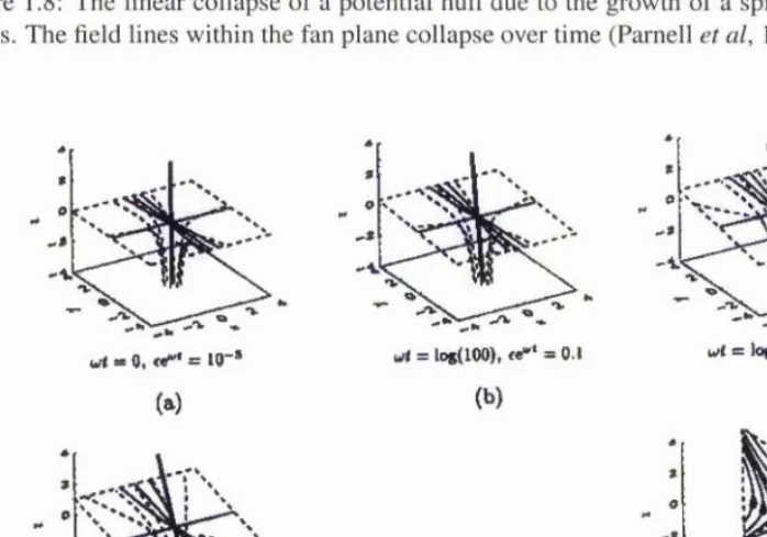
Figure 1.8: The linear collapse of a potential null due to the growth of a spine current along the z-axis. The field lines within the fan plane collapse over time (Parnell et al, 1997).

» 0, <*-' = 10 ' (a)

ut = log(I00), <*r‘ = 0.1

(b)

ut = log(200), <*-' - 0.2

(c)

velocity

ut = log(300), <«-' = 0.3

(d)

1.4 Null Point Collapse in Three Dimensions 21

1.4.3 Non-Linear Collapse

The non-linear collapse of a three-dimensional null with incompressible plasma flow was studied by Bulanov and Olshanetsky (1984), They looked at the non-linear evolution of the incompressible MHD equations. They expressed the plasma flow, magnetic field and pressure in the form v =

'W(t)r and derived an equation for the deformation matrix where W = with an overdot denoting the time derivative.

(M '^ r^ n o ) , MB^O) - { M B { 0 ) M - Y M B { 0 )

^ = ---5273--- + ---D--- '

where D denotes detvW. They investigated the special case where

B (1.46)

/ Bii B\2 0 \

B21 B22 0

\ 0 0 B33 J

( M\i M\2 0

M = M21 M22 0 I , (1.47)

\ 0 0 M33

and found that a finite time singularity (at t = to) was formed in the solution. As i fo, the asymptotic behaviour of the variables is

B oc {t — to)~^/^, yV (X (t - to)~^, D (X {t - to)~‘^^^. (1.48)

Bulanov and Sakai (1997, 1998) gave a more complete account of the incompressible col­ lapse of null points. In their paper of 1997, using the same system of equations as Bulanov and Olshanetsky (1984) they derived the non-linear equations

V l l + “^11 + ‘^12^21 — { B\2 — B 2l ) B2l , (1.49)

V i2 = { B i2- B 2i ) B22, (1.50)

= — { B i2- B 2i ) B u , (1.51)

V 3 3 + ^33 = 0, (1.52)

B n + B 1 2 V 2 1 — V 1 2 B 2 1 =0, (1.53)

B i2 + B 1 1 V 1 2 — 2 B 1 2 U 1 1 — V 1 2 B 2 2 = 0, (1.54)

1.4 Null Point Collapse in Three Dimensions 22

(C )

X 3

Figure 1.10: The non-linear collapse of a potential null point due to growth of the spine current, causing the spine to flatten out. (Bulanov and Sakai, 1997)

Figure 1.11: The non-linear collapse of a potential null point due to the growth of the fan current, causing the spine to collapse into the fan plane. (Bulanov and Sakai, 1997)

V22 + V21V12 — V2lBi2 = 0. (1.56)

They started with a potential null point and considered two different cases. In the first case, the perturbation of the flow was parallel to the fan plane of the null, causing spine current density to grow (see Figure 1.10). The spine flattened out and rotated, eventually forming a line of two- dimensional X-points. In the second case, the flow perturbation was parallel to the spine of the null, causing the fan current to grow. The spine collapsed into the fan plane, like a falling tree. The fan plane also changed its position slightly, ending up inclined at a slight angle to its original position as can be seen in Figure 1.11. In their paper of 1998, they extended their analysis to a weakly ionised plasma.

1.5 Magnetic Annihilation in Two Dimensions 23

1.5 Magnetic Annihilation in Two Dimensions

1.5.1 Introduction

Annihilation of a magnetic field is a natural way of converting stored magnetic energy into heat through ohmic dissipation. One of the useful features of annihilation models is that they allow us to study clearly the physical process of energy conversion, one of the ingredients of the more complex phenomenon of magnetic reconnection (e.g., Priest and Forbes, 2000).

1.5.2 Simple Annihilation

Let us assume first that the magnetic Reynolds number for a plasma flow is much smaller than unity, which happens in a cunent sheet with very small width and non-vanishing diffusivity. We can then reduce the induction equation to the following form

^ (1.57)

Consider a one-dimensional field which initially has a uniform, positive value (Bq) for æ > 0 and

a uniform negative value (~-Bq) for a; < 0. As time passes, the field will dissipate, starting from the origin (Figure 1.12). The appropriate solution to the induction equation under these conditions is

rx/{Ar}tŸf^

B{x^t) = —rjT; / exp(-w^)(itt. (1.58)

Jo

The total magnetic flux remains zero due to the symmetry of the solution, since there are equal and opposite amounts on both sides of the central null so that they sum to zero. The total current.

J= f j d x = — , (1.59)

J

is constant and the current just spreads out in space as the current sheet broadens in time. The magnetic energy, however, decreases at a rate

r°° B^ dt

/

oo

poo

—— dx — ~ I —dx, (1.60)

-oo

J —oo ^

1.5 Magnetic Annihilation in Two Dimensions 24

Figure 1.12: The ohmic decay of a simple current sheet with a one-dimensional magnetic field

B{x, t)y. The initial field profile is the black line, the blue line represents the profile at f = 1/4, the green line at f = 7/4 and the red line at f = 49/4.

1.5.3 Stagnation-Point Flow Model

Sonnerup and Priest (1975), building on earlier work by Parker (1973), discovered an exact solu­ tion to the steady-state, incompressible MHD equations for a plasma flow of the form

-- VqX 'U'li — voy

a a

acting on a one-dimensional magnetic field in the y- direction of the form

B = B{x)y.

Integrating the induction equation gives us

E + V X B = ryV x B, _(1.61)

where E = Ez is a constant in two dimensions (x, y) due to Faraday’s law. Substituting the field

and velocity into Equation (1.61) yields an ordinary differential equation for the unknown B{x),

namely.

a dx

It may be integrated to give

VqI

(1.62)

1.5 Magnetic Annihilation in Two Dimensions 25

ail

-0.5 0.5

-2

-0 .1

-2 4

X

Figure 1.13: The stagnation-point flow model for magnetic annihilation. {Left) The velocity stream lines (thick) and the magnetic field lines (thin). The shaded region denotes the diffusion region. (Right) A plot of the field strength (B) as a function of distance x.

where P = 2ar]/vo and

daw(^) = exp(—^^)

f

Jo

This represents a hyperbolic plasma flow into the null point along the rr-axis and out from the null point along the y-axis. The flow advects the magnetic field lines in towards the stagnation point where they concentrate, causing a current concentration to be formed, before diffusing across the y-axis to annihilate with the field lines from the other side. Figure 1.13 shows the field lines and stream lines of the solution, and also how the field strength varies with distance from the null.

There is, however a limit on how fast the magnetic field can be annihilated. The equation of motion implies

and so determines the plasma pressure as

.2 ^ 2

(1.64)

P = P s - pv‘

2/io ’ (1.65)

where Ps is the pressure at the stagnation point. The pressure must always be greater than zero, and so this puts a constraint on the maximum rate of annihilation of the field (Priest, 1996; Litvinenko

et al, 1996) or the plasma beta (the ratio of the plasma pressure to the magnetic pressure. Jardine

et al, 1993). The requirement that the pressure be positive can be written as

1.5 Magnetic Annihilation in Two Dimensions 26

where M , is the external Alfvén Mach number, is the external plasma beta and Rme is the magnetic Reynolds number. The external values are calculated far from the null at a position

1.5.4 Time-Dependent Stagnation-Point Flow

If the stagnation-point flow is generalised to become

v = ^ ( æ , ~ y ) , (1.67)

and the magnetic field becomes

B = [B*(!/,().0], (1.68)

then the induction equation reduces to

Scaling away r} and a, and making the substitutions

Y = yg{t), - = g ,

Equation (1.69) becomes

where / = v/g^. This can be solved to give the time-development of an initial magnetic field,

B{Yf0) = Bo(y) in the form

a (y 'T ) = (1.71)

1,5 Magnetic Annihilation in Two Dimensions 27

(a)

t-7.0

energy

grad

8

0 I 8 3 *

(b)

maxy

grad maxB energy

(a)

Figure 1.14: Time-dependent magnetic annihilation. (Top) The initial profile

1.5 Magnetic Annihilation in Two Dimensions 28

1.5.5 Reconnective Annihilation

The steady stagnation-point flow solution was generalised by Craig and Henton (1995), who con­ sidered a two-dimensional velocity

Vx — —a;, Vy = y T’(aj),

which satisfies V - v = 0 and a magnetic field of the form

B = Av -f- G{x)y

which satisfies V ■ B = 0. The stagnation-point flow is therefore modified by the addition of a simple shear in the ^-direction. The corresponding magnetic flux function (A) and stream function

i'lp) are given by

A - X x y + g{x), 'i/j= xy + Xg{x),

where F{x) — —A dgfdx and G{x) = (1 — A^) dg/dx. F{x) and G{x) are related by

For this form of solution Equation (1.62) reduces to

which determines G{x) as

,1.73,

A is a measure of how far this solution is from the stagnation-point flow solution (which is given by A = 0). This solution allows one to impose the values of three of the four vector components of V and B at some external point. The fourth is determined by the solution in terms of the other three.

This model does not represent genuine reconnection since the current sheet is purely one­ dimensional and the magnetic field just diffuses or annihilates across the y-axis (Figure 1.15). It is therefore referred to as reconnective annihilation. The field lines are advected in towards the null and, as in simple annihilation, they diffuse together.

1.6 Reconnective Magnetic Annihilation in Three Dimensions 29

1.0

0.5

0.0

-0.5

- 1.0

0.5 0.0

X

-0.5

- 1.0

Figure 1.15: The streamlines (dashed) and the field lines (solid) for two-dimensional reconnective annihilation. The diffusion region is shaded grey and the arrows indicate the direction of the field and flow, both inflowing on the boundary. (Priest ef al, 2000)

functions in the form

A = Ao{x) + Ai{x)y, ip = 'ipo(x)'ipi{x)y,

to model the magnetic field and plasma flow. Such an approach yields an extra parameter, 7,

which allows three different types of solution in the outer advection region. 7 < 1 produces

trigonometric solutions, 7 = 1 has solutions like the previous Craig-Henton (1995) solution and 7 > 1 yields hyperbolic solutions.

This form of solution represents physically the same kind of annihilation as the Craig-Henton (1995) solution, but it is a two-fold generalisation in that it allows us to impose all four of the boundary values (Vx, Vy, Bx, By) at an external point, as well as the value of 7, whereas the Craig-Henton (1995) solution would only allow three of the four boundary values to be imposed.

1.6 Reconnective Magnetic Annihilation in Three Dimensions

1.6.1 Introduction

1.6 Reconnective Magnetic Annihilation in Three Dimensions________________________^

no exact solutions for spine or fan reconnection exist. However, Craig and co-workers have suc­ ceeded in discovering exact solutions for three-dimensional reconnective annihilation which are similar in spirit to the reconnective annihilation solutions in two dimensions and which possess one-dimensional current concentrations stretching along either the spine or the fan. The limitation of their model, as of the stagnation-point flow model, is that the current concentrations are not bounded but extend to infinity.

1.6.2 Fan Annihilation

Craig et al (1995) extended the idea of reconnective annihilation into three dimensions. They modelled a sheared stagnation-point flow of the form

Vx — Xf Vy — K y Fyix'), Vz — (1 K^z Fz (a:),

with a magnetic field

B = Av + G y { x ) y + Gz{x)2,.

This allowed them to consider annihilation in the fan plane of a null point. There was again the relationship

and they could solve the differential equations

xG'y + KGy = - Y ^ G ' y > (1.74)

xG', + (1 - K )G , = - (1.75)

to determine the structure of the magnetic field and plasma flow. The fan is given by the plane æ = 0 and the spine is inclined such that

_

^

\ n

( i + K

) '

X n { 2 ~ K ) '

1.7 Summary 31

(b)

o

Figure 1,16: The advection of field lines across the spine of a null point in a model of fan recon­ nective annihilation. The same plasma element is followed and one can see that a field line frozen into the plasma crosses the spine and diffuses in the fan. (Craig et al, 1995)

1.6.3 Spine Annihilation

Craig and Fabling (1996) later modelled annihilation occurring along the spine line of a null point. They used cylindrical polar coordinates and considered a plasma velocity and magnetic field of the form

= Vz ~ \f{ R )s m (j} - az,

Br — , Bz = f{R)sm(p — Xaz,

where f{R) satisfies

(1.77)

(1.78)

(1.79)

and / ' = df/dR. This yielded a cylindrical diffusion region around the spine of radius ~

The field close to the spine grows linearly with R and drops off far from the spine and diffusion

region as R~'^.

1.7 Summary

1.7 Summary__________________________________________________________________^

subject to collapse. The linear and non-linear collapse properties have been determined, and in the absence of dissipative terms the collapse results in a current sheet being formed at the null. Adding the effect of diffusivity or other non-ideal effects allows the collapsing current to dissipate, releasing energy as the magnetic field annihilates or reconnects.

This chapter has been concerned with the exact MHD solutions for collapse, annihilation and reconnective annihilation models in two and three dimensions. The theory of reconnection has been discussed extensively elsewhere (e.g.. Priest and Forbes, 2000). Reconnective annihilation has more features in common with the simple annihilation models, and can be thought of as a generalisation of them. The annihilation rate in these models may occur at any rate up to a beta- limited value, depending on the inflow velocity of the plasma and field to the diffusion region. In the annihilation models, the plasma acceleration due to a pressure gradient along the current sheet is passive, due to the stagnation point flow. In genuine reconnection on the other hand, this acceleration is due to a combination of the Lorentz force and an excess plasma pressure in a sheet of finite length.

The MHD equations are highly non-linear and so exact solutions are extremely rare. Until ten years ago only the Imshenik and Syrovatsky (1967) collapse solution and the steady stagnation- point flow annihilation solution were known, but a combination of ingenuity and good fortune has now produced a series of generalisations of these. Such exact solutions are invaluable in highlighting the basic physical processes in a transparent manner and may form the basis for more complex approximate and computational studies of the fundamental processes of null collapse, magnetic annihilation and magnetic reconnection both in two dimensions and in three dimensions.

Chapter 2

Stagnation-Point Flow and Asymmetric

Boundary Conditions

fw# ^ f w A »