Hyper volume evolutionary algorithm

(1)

Hyper-volume Evolutionary Algorithm

Khoi Nguyen Le

1,∗

, Dario Landa-Silva

2 1_{VNU University of Engineering and Technology, Hanoi, Vietnam}

2_{The University of Nottingham, Nottingham, United Kingdom}

Abstract

We propose a multi-objective evolutionary algorithm (MOEA), named the Hyper-volume Evolutionary Algorithm (HVEA). The algorithm is characterised by three components. First, individual fitness evaluation depends on the current Pareto front, specifically on the ratio of its dominated hyper-volume to the current Pareto front hyper-volume, hence giving an indication of how close the individual is to the current Pareto front. Second, a ranking strategy classifies individuals based on their fitness instead of Pareto dominance, individuals within the same rank are non guaranteed to be mutually non-dominated. Third, a crowding assignment mechanism that

adapts according to the individual’s neighbouring area, controlled by the neighbouring area radius parameter,

and the archive of non-dominated solutions. We perform extensive experiments on the multiple 0/1 knapsack

problem using different greedy repair methods to compare the performance of HVEA to other MOEAs including

NSGA2, SEAMO2, SPEA2, IBEA and MOEA/D. This paper shows that by tuning the neighbouring area

radiusparameter, the performance of the proposed HVEA can be pushed towards better convergence, diversity or

coverage and this could be beneficial to different types of problems.

Received 05 December 2015, revised 20 December 2015, accepted 31 December 2015

Keywords: Multi-objective Evolutionary Algorithm, Pareto Optimisation, Hyper-volume, Knapsack Problem.

1. Introduction

The development of heuristic and evolutionary techniques to solve real-world multi-objective

optimisation problems is an an active

research area. In Pareto-based multi-objective optimisation, a set of non-dominated solutions,

also known as Pareto front, is sought so

that the decision-maker can select the most

appropriate one. Evolutionary xalgorithms

and other population based heuristics seem well suited to deal with Pareto based multi-objective optimisation problems because they can evolve a population of solutions towards the

Pareto-optimal front in a single run. A good

multi-objective evolutionary algorithm (MOEA) should be able to obtain Pareto fronts that are both well-distributed and well-converged.

∗

Corresponding author. Email: [email protected]

An important issue in a MOEA is how to establish superiority between solutions within

the population, i.e. how to assess solution

fitness in a multi-objective sense. In this paper, we proposed the Hyper-Volume Evolutionary Algorithm (HVEA), a MOEA that employs the concepts of volume dominance proposed by Le et at [1] to assess solution fitness in multi-objective optimisation.

The paper is organised as follows. Section 2

describes the HVEA algorithm. In Section 3,

most well-known and recent MOEAs in the literature together with the multiple 0/1 knapsack

problem are discussed. In Section 4, the

experimental results and discussion are presented. Then some conclusions and perspectives are discussed in Section 5.

(2)

2. Hyper-volume Evolutionary Algorithm

We propose a new approach to multi-objective

optimisation, the Hyper-volume Evolutionary

Algorithm (HVEA). HVEA deploys techniques that are well established in the literature as well as presents new ones in order to find the Pareto front of the problem. As other population-based MOEAs, the proposed HVEA

• Uses a population of current solutions and an archive for storing the best solutions found so far,

• Assigns scalar fitness values to individuals and uses the Pareto dominance relationship,

• Employs a crowding strategy to maintain the diversity of the population and, if necessary, control the size of the archive during the search.

However, HVEA is distinguished by

four features:

• The fitness of an individual is calculated using the hyper-volume of that individual

and the hyper-volume of the current

representative Pareto front.

• Individuals are ranked based on their

fitness values, individuals having fractional difference in fitness values between them are classified into the same rank.

• A niching technique to preserve the diversity of the population based on distance between the individual and other solutions in its neighbouring area.

• Offspring that improve the current Pareto front (in other words offspring that dominate individuals in the current Pareto set) are guaranteed to be selected not only for the archive but also for the tournament selection to fill the mating pool.

Overall, HVEA works as follows:

Step 1: Initialisation: Start with an empty populationPand create an initial archive P

(each of sizeN).

Step 2: Fitness assignment: Calculate

fitness values of individuals in PS_P

(cf. Section 2.1).

Step 3: Ranking assignment: Assign ranking to individuals inPS

P(cf. Section 2.2).

Step 4: Environmental selection: Repeatedly copy all individuals having the best ranking fromPtoPand assign their crowding values until the size ofPexceedsNthen reduce the size ofPby means of the truncation operator (cf. Section 2.3andSection 2.4).

Step 5: Termination: Stopping criteria are satisfied then present all non-dominated individuals inPas solutions to the problem, and then the algorithm stops here.

Step 6: Generating offspring: Apply crossover and mutation operators on parents, which are selected with binary tournaments, to produce offspring (cf. Section 2.5). Go to Step 2.

2.1. Fitness Assignment

The fitness assignment procedure of HVEA deploys the concept of volume dominance proposed by Le et at [1]. Le et at. proposed a new relaxed Pareto dominance for multi-objective optimisation, named volume dominance. They

assign strength values to individuals in the

(3)

set of all individuals in ParetoFrontthat Pareto-dominatex.

RP(x)=

x*|x* x^x* ∈ParetoFront

(1)

xref_i =sup

fi(x*)|x*∈RP(x)

(2)

Vref(x) is the hyper-volume of xref, given by (2), w.r.t. the reference pointr~x, given by (4), then the fitness value of individualxis as follows:

f itness(x)=1− V(x)

Vref₍_x₎ (3)

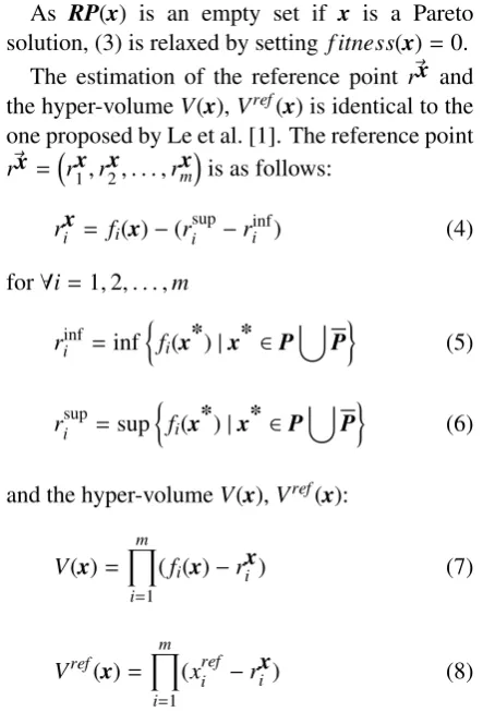
As RP(x) is an empty set if x is a Pareto solution, (3) is relaxed by setting f itness(x)=0.

The estimation of the reference point r~x and the hyper-volumeV(x),Vref(x) is identical to the one proposed by Le et al. [1]. The reference point

~

rx =rx₁,r₂x, . . . ,rx_mis as follows:

r_ix= fi(x)−(rsup_i −rinfi ) (4)

for∀i=1,2, . . . ,m

r_iinf =inf

fi(x*)|x* ∈P

[ P

(5)

r_isup=sup

fi(x*)|x* ∈P

[ P

(6)

and the hyper-volumeV(x),Vref(x):

V(x)= m

Y

i=1

(fi(x)−rxi ) (7)

Vref(x)= m

Y

i=1

[image:3.595.319.513.113.247.2]

(xref_i −r_ix) (8)

Fig. 1 illustrates the estimation of the above terms that are required for the calculation of individual fitness in HVEA. Lower values of f itness(x) are preferred. The procedure to determine the fitness values of individuals in the offspring population P and the archive P is as follows:

f1 f2

O

Pareto front sup

r

inf

r x

r

current Pareto front representative

Pareto front

xref x

[image:3.595.68.290.310.637.2]

V(x) Vref_(x)

Fig. 1: The fitness assignment in HVEA.

Step 1: Use all individuals inPandPto update:

~

rinf =_rinf

1 ,rinf2 , . . . ,rinfm

(9)

~

rsup=_rsup 1 ,r

sup 2 , . . . ,r

sup

m

(10)

whererinf_i andrsup_i are given by (5) and (6) respectively.

Step 2: Update ParetoFront using all newly generated offspring in P. Assign fitness

value of −1 to offspring that

Pareto-dominate at least one individual in

ParetoFront of the previous generation.

Assign fitness value of 0 to the remaining individuals in ParetoFront of the current generation. Apply (3) to assign fitness value to all remaining individuals inPandP.

Assigning fitness value of −1 to offspring

that Pareto-dominate at least one individual

in ParetoFront enables HVEA to distinguish

individuals that make a direct contribution in moving the Pareto front forward during the environmental selection and mating selection. This fitness assignment strategy emphasises the idea of preferring individuals near the Pareto front especially individuals that improve the Pareto front of the previous generation.

2.2. Ranking Assignment

(4)

classifies individuals with similar (or identical) characteristic(s) into the same category(ies). The characteristic usually used is the Pareto

non-dominance. In other words, Pareto

non-dominated individuals are classified into one category (rank). Therefore it is guaranteed that individuals with the same rank are all mutually non-dominated. An example is NSGA2 [2] with its fast non-dominated sorting approach. HVEA takes a paradigm shift in ranking individuals. In HVEA, it is the case that an individual is Pareto dominated by another individual having the same

rank. The main intention of this mechanism

is to allow slightly worse quality individuals to be able to compete for survival and/or selection. HVEA computes ranking from the individual fitness value as follows:

rank(x)=

$

f itness(x)× 1

µ

%

(11)

where parameter µ indicates the ‘size’ of each ranking level whereas 1_µ could be referred as the desired number of ranks (desired number

of ‘fronts’). The advantage of this ranking

assignment mechanism is that only Pareto non-dominated individuals are assigned rank 0 with exception of individuals, which improve the Pareto front, are assigned rank−1. Other Pareto dominated individuals are assigned rank with some noise induction by applying (11).

2.3. Environmental Selection

LetFi is the set of individuals in PSPwith rank(x)=i:

Fi =

n

x|rank(x)=i∧x∈P[Po (12)

One set at a time, all individuals from each set Fi, with i = −1,0,1,2, . . ., are copied to the archive P until the size of P equals to

or exceeds N. If the size of P equals to N,

the environmental selection is completed.

Otherwise, individuals in the last frontFl copied toP, are removed fromPuntil reducing the size of Pto N. The last copied front Fl satisfies the following conditions:

l−1

X

i=−1

|Fi|<N (13)

l−1

X

i=−1

|Fi|+|Fl|>N (14)

Individuals inFl are sorted by their crowding values. The individual with the highest crowding

value in Fl is removed from P and Fl. The

crowding value of remaining individuals inP, not justFl, are updated accordingly. These processes are repeated until the size ofPequals toN.

2.4. Crowding Assignment

As NSGA2 and SPEA2, HVEA employs the distance-based approach to estimate the

density of individuals around a particular

individual. However HVEA’s crowding

assignment mechanism is different from NSGA2

and SPEA2. Both NSGA2 and SPEA2 only

consider “one neighbour” in the neighbouring area in order to determine the density of a

particular individual. NSGA2 combines the

distance to the adjacent neighbour in each objective to estimate the crowding of a particular individual whereas SPEA2 considers the distance

to the k-th nearest neighbour. HVEA takes

into account all individuals in the neighbouring area to determine the crowding of a particular

individual. The neighbouring area is defined

by the current state of the combined population

PS

Pand aradiusω. An individualx* is in the neighbouring area of an individual x (in other word x* and x are neighbours) if the following condition is satisfied:

xi−x

∗

i

≤

rsup_i −rinf_i ×ω (15)

for ∀i = 1,2, . . . ,m and rinf_i and rsup_i are given in (5) and (6). Let NB(x) is the set of all neighbouring individuals of x that means x* ∈

NB(x) if and only ifx* andx are satisfied (15). Then, the crowding value ofxis as follows:

crowding(x)= X

x*∈NB(x)

(d(x,x*)+1)−1(16)

whered(x,x*) is the Euclidean distance between

xandx*:

d(x,x*)=

v t m

X

i=1

(5)

and lower value ofcrowding(x) is preferred. Apart from considering all individuals in the neighbouring areato estimate the crowding of a particular individual, another main difference in crowding assignment mechanism between HVEA and NSGA2, SPEA2 is that NSGA2 only uses each front separately to estimate crowding value of individuals in that front, SPEA2 uses all individuals in both the offspring population P

and the archive Pto estimate crowding value of individuals, but HVEA only uses individuals in fronts, which are already added to the archiveP, to estimate the crowding value. Additionally, the crowding value of individualx ∈ Pis repeatedly adjusted when a new frontFiis added toPwhich is not the case in SPEA2. The pseudocode for the crowding assignment of frontFi (−1 ≤ i ≤ l) is as follows:

ProcedureCrowdingAssignment(Fi) begin

foreachxinFi

foreachx*inFi(x*,x) ifx*andxare neighbours

thenadd (d(x,x*)+1)−1_to_crowding_{(x) and}_crowding_(x*) endif

endfor

foreach frontFj(−1≤j<i) foreachx*inFj

ifx*andxare neighbours

thenadd (d(x,x*)+1)−1_to_crowding_{(x) and}_crowding_(x*) endif

endfor endfor endfor end

2.5. Generating Offspring

HVEA chooses parents to fill the mating pool

by binary tournament selection. Individuals

competed for the second parent are different

from the first parent. The binary tournament

selection prioritises the following order: ranking, crowding,fitnessvalues of individuals. Crossover and mutation are applied on the mating pool

to form the offspring population P. Any

duplicated offspring dies out of the combined

population PS

P. This guarantees that there is no duplication in the combined population

PS

P before the environmental selection

process. Consequently, there is no duplication in the archiveP.

3. Comparative Case Study

3.1. Multi-objective Evolutionary Algorithms

The performance of HVEA is compared to NSGA2 [2], SEAMO2 [3], SPEA2 [4], IBEA [5] and MOEA/D [6].

3.1.1. Non-dominated Sorting Genetic Algorithm 2 (NSGA2)

Deb et at. [2] used a fixed population and

a fixed archive of size N for their NSGA2.

They proposed a fast non-dominated sorting approach in NGSA2 to classify individuals in a population into different non-domination levels or different fronts. NSGA2 employed a density estimation metric to preserve the population diversity. It required to sort each front according to each objective function value in ascending order of magnitude. The boundary individuals are assigned an infinite distance value. The density of individuals surrounding other intermediate individual in the front is the sum of the average normalised distance of two individuals on either side of this individuals along each of the

objectives. The mating pool is filled by the

binary tournament selection with the following priority, non-domination level then crowding distance. The offspring population is formed by applying crossover and mutation on the mating pool. The best fronts of the offspring population and the archive combined are selected for the next archive. If the size of the archive is greater than N, individuals in the last front is removed to reduce the size of the archive to N based on their crowding value. There is no treatment to prevent duplication of individuals whilst forming the archive. The duplication individuals could be spotted by the crowding value and removed during the truncation of the archive but it is not exhaustive.

3.1.2. Simple Evolutionary Algorithm for Multi-objective Optimization 2 (SEAMO2)

(6)

Crossover and mutation is applied on the pair of parents to produce offspring. The offspring replaces one of the parents if either its objective

vector improves on any best-so-far objective

function or it dominates that parent. If neither the offspring dominates the parents nor the parents dominate the offspring, the offspring replaces a random individual in the population that the

offspring dominates. SEAMO2 does not allow

duplication in its population. Therefore,

any duplicated offspring dies before the

replacement process.

3.1.3. Strength Pareto Evolutionary Algorithm 2 (SPEA2)

Zitzler et at. [4] employed a fixed size archive to store non-dominated individuals in addition

to a population for SPEA2. SPEA2 uses a

fine-grained fitness assignment strategy which takes for each individual into account how many individuals it dominates and it is dominated

by. Each individual in both the archive and

the population is assigned a strength value S(i), indicating the number of individuals it dominated. The raw fitnessR(i) of an individual is defined as the sum of the strength value of all individuals by which it is dominated.

S(i)=

n

j| j∈P[P∧i jo

(18)

R(i)= X

j∈PSP_∧_j_i

S(j) (19)

SPEA2 uses an adaptation of the k-th nearest neighbour method to estimate the density of an

individuals. The density of an individual is

estimated as the inverse of the distance to the k-th nearest neighbour. Then, the density is added to the raw fitness Ri to yields the fitness of an individual i. Similarly to NSGA2, SPEA2 fills the mating pool using binary tournament selection on the archive based on the fitness of individuals participated in the tournament. Crossover and mutation is applied on the mating pool to create the offspring population. From the offspring and the archive population, all individuals having fitness less than one, i.e. all

non-dominated individuals in PS

P, are copied to the next archive. Zitzler et at. pointed out that there are two situation: either the archive

is too small or too large. If the archive is

too small, the best dominated individuals, based on the fitness value, are copied to fill P. In the later situation, non-dominated individuals in the archive are iteratively removed until the archive’s size is not exceeded. The removal of non-dominated individuals from the archive is carefully managed by using an archive truncation method that guarantees the preservation of boundary solutions. As in NSGA2, SPEA2 relies on the archive truncation to remove duplicated individuals but it does not guarantee that the archive contains no duplication.

3.1.4. Indicator Based Evolutionary Algorithm (IBEA)

Zitzler and K¨unzli [5] proposed a general

framework indicator-based evolutionary

algorithm (IBEA). IBEA could be referred as classic MOEAs but guided by a general

preference information of the dominance

relationship, a binary quality indicator. IBEA needs neither specifications of weights or targets (as in aggregation methods) nor the dominance relationship and distribution techniques (as

in classic MOEAs). IBEA uses this binary

indicator guiding the search to optimise the approximation set. The binary quality indicator in IBEA maps an ordered pair of individuals to a real number which therefore could be used for fitness calculation. Zitzler and K¨unzli [5] proposed two indicators, the additive -indicator I+ and the hyper-volume-indicatorIHD. For an order pair of individuals (x1_,_x2_),_I

+(x1_,_x2_{) gives}

minimum distance for which x1 is translated

in each in objective space to weakly dominate

x2. IHD(x1,x2) measures the space volume that is dominated by x2 but not by x1 with respect

to a predefined reference point. The fitness

of an individual is estimated as the sum of an exponential function of the indicator values.

A positive constant κ = 0.05 is applied to

(7)

is suggested to use adaptive scaling for both indicator values and objective values to avoid the issue of estimating a good reference point. As aforementioned population based MOEAs (NSGA2 and SPEA2), IBEA uses a fixed size archive and an offspring population. Offspring is produced by recombination and mutation on a pair of parents selected from the archive. The archive and the offspring population is combined and truncated to generate the new archive for the next iteration.

3.1.5. Multi-objective Evolutionary Algorithm

Based on Decomposition (MOEA/D)

MOEA/D, proposed by Zhang and Li [6],

decomposes a multi-objective optimisation

problem into a number of scalar optimisation sub-problems and optimises them simultaneously. Each sub-problem is optimised by utilising information from it neighbouring sub-problems.

Non-dominated individuals found during

the search are stored to an external archive. MOEA/D predefines a set of even spread weight vector nλ1, . . . , λNo, where N is the number of sub-problems, or the population size of MOEA/D. Each sub-problem ith corresponds to a weight vectorλi. The neighbourhood of theith sub-problem consists of all sub-problems with the weight vectors closest toλiwhich include the ith sub-problem itself. Then, the population of MOEA/D consists the best solution xi found so far for each sub-problem ith. At each iteration, an offspring to ith sub-problem is produced by recombination and mutation on parents which are the current solutions to the neighbohood of the ith sub-problem. The offspring replaces current solutions of the ith sub-problem and its neighbouring sub-problems if the fitness value of the offspring is better than that of these current solutions. See [6] for more details of MOEA/D and the fitness calculation.

3.1.6. Adaptive Evolutionary Multi-objective

Simulated Annealing (EMOSA) [7]

Li and Landa-Silva [7] proposed an improved

version of MOEA/D by incorporating an

advanced local search technique (simulated

annealing) and adapting the weight vectors, so called EMOSA. EMOSA deploys the cooling technique in simulated annealing to adaptively modified weight vectors at the lowest temperature in order to diversify the population towards the unexplored part of the search space. EMOSA also uses simulated annealing technique to further improve each individual in the population.

Finally, EMOSA use -dominance to update

the external population in order to maintain the diversity of the external population. The performance of EMOSA is then compared

against a set of multi-objective simulated

annealing algorithms and a set of multi-objective memetic algorithms using multi-objective 0/1 knapsack problem and multi-objective travelling salesman problem. EMOSA performs better than all these algorithms and is capable of finding very good distribution of non-dominated solutions.

3.1.7. S-Metric Selection EMOA (SMS-EMOA)

SMS-EMOA is a steady state population and selection scheme, proposed by Beume et al. [8]. SMS-EMOA’s goal is to maximise the hyper-volume, S-metric value, of the population by

removing an individual which exclusively

contributes the least hyper-volume. At

each iteration, an offspring is produced by

recombination and mutation. The offspring

replace an individual in the population Pt if it leads to higher quality of the population with respect to theS-metric. The resulting population

Pt+1, formed by combining the offspring and

the previous population Pt, is partition into different non-dominated sets, fronts, using the fast non-dominated sorting algorithm as describe in NSGA2 [2]. The first front R1 contains all

non-dominated solutions ofPt+1, the second front

contains all individual that are non-dominated in the set (Pt+1\R1), etc.. An individual r is

discarded from the last frontRv, the worst ranked front, for which that individual exclusively contributes the least hyper-volume to the last frontRv.

r=arg min s∈Rv

[∆S(s,Rv)] (20)

(8)

Beume et al. also investigated several selection variants of SMS-EMOA and pointed out that if there is more than one front in Pt+1 (v >

1), the individual with the most number of

dominating points should be discarded. The

equation (20) should be replaced by the following equation (22):

r=arg max s∈Rv

[d(s,Pt+1)] (22)

d(s,Pt)=|{y∈Pt|y≺ s}| (23)

The main motivation of this selection variant is to reduce the runtime complexity and to emphasise on sparsely filled regions of the solution space. It is expected that dominating individual will rise in rank to better fronts and fill those vacancies [8]. The experimental results on continuous problems including ZDT and DTLZ indicated that SMS-EMOA outperforms NSGA2 and SPEA2.

It is emphasised that HVEA is clearly different from SMS-EMOA. SMS-EMOA uses the exclusive hyper-volume contribution of individuals in the worst front to eliminate an individual during the steady-state selection

scheme. HVEA use the hyper-volume of

an individual to determine its fitness and

its ranking. The next archive is selected

from the archive population combining with the offspring population using only individual ranking and crowding.

3.1.8. Direction-based Multi-objective Evolutionary Algorithm (DMEA)

Bui et al. [9] proposed a population-based evolutionary algorithm that evolves a population along directions of improvement. They are two types of directions employed in DMEA i.e. (1) the convergence direction between an archived non-dominated solution and a dominated solution from the parental pool and (2) spread direction between two non-dominated solutions in the archive. These directions are used to perturb the parental population at each generation. A half of the next-generation parental pool is formed by non-dominated whose spread is aided

by a niching criterion applied in the decision space (i.e. using spread direction), whereas the other half is filled by non-dominated dominated solutions from the combined population using convergence direction. The archive is updated by scanning a bundle of rays from the estimated ideal point into the part of objective space containing the current pareto front. For each ray scanned, the non-dominated solution in the combined population, which are closest to the ray, is selected for the next archive. The experimental result on continuous problems including ZDT and DTLZ obtained by DMEA is slightly better than those by NSGA2 and SPEA2.

3.1.9. Direction-based Multi-objective Evolutionary Algorithm II (DMEA-II)

The DMEA is further improved and so

called DMEA-II [10]. The main differences

between these two algorithms are: (1) an

adaptive approach for choosing directional types in forming the parental pool, (2) a new concept for ray-based density for niching and (3) a new selection scheme based on this ray-based density. In DMEA, a half of the parental pool is formed by using the convergence direction and the other half is formed by using the spread direction. DMEA-II deployed an adaptive approach, in which this ratio is depended on the number of non-dominated solutions in the current

population. The higher the number of

non-dominated solutions in the current population is, the more use of the spread direction. In other words, if the current population contains all non-dominated solutions then the spread direction is used to generate the whole parental population. The second improvement is a new ray-based density approach by counting the number of ray that a solution is the closest one. Then a half of the archive is updated by non-dominated solutions with highest ray-based density, whereas the other half is formed by solutions closest to each ray. Continuous problems including ZDT, DTLZ and UF are used as benchmark problems

for comparison. Experimental results show

(9)

3.2. Experimental Design

3.2.1. Multi-objective Optimisation Problem The performance of HVEA is assessed by comparing to NSGA2, SEAMO2, SPEA2, IBEA and MOEA/D on the multiple 0/1 knapsack problem proposed by Zitzler and Thiele [11]. The multiple 0/1 knapsack is defined as a set ofn items and a set ofmknapsacks, weight and profit associated with each item in a knapsack, and an upper bound for the knapsack capacity. The goal is to find a subset of items that maximise the profit in each knapsack and the knapsack weight does not exceed its capacity.

pi,j=profit of item jin knapsacki

wi,j =weight of item jin knapsacki

ci=capacity of knapsacki

find a vector x = (x₁,x₂, . . . ,xn) ∈ {0,1}n such that:

∀i∈ {1,2, . . . ,m}: n

X

j=1

wi,j×xj≤ci (24)

and maximise f(x) = (f1(x),f1(x), . . . , fm(x)), where

fi(x)= n

X

j=1

pi,j×xj (25)

andxj =1 if and only if item jis selected. There are 9 instances for the multiple 0/1 knapsack problem [11]. The population size for each instance is as follows:

We perform 50 independent runs for statistical analysis, each run is of 2000 generations. It is noticed that MOEA/D predefines the set of even spread weight vector nλ1, . . . , λNo where N = Cm_H−₊1_m₋₁ (H: controlling parameter). It is difficult to change N to the required population size. Therefore it is suggested to respect the population size set by MOEA/D but alter the number of generations for MOEA/D as follows

g=

_S

N ×2000

(26)

Table 1: Parameter Setting for The Multiple 0/1 Knapsack Problem

Instance Population Size (S) N in MOEA/D

ks2 250 150 150

ks2 500 200 200

ks2 750 250 250

ks3 250 200 351

ks3 500 250 351

ks3 750 300 351

ks4 250 250 455

ks4 500 300 455

ks4 750 350 455

There are several representations, repair

methods and offspring productions for the

multiple 0/1 knapsack problem. Our preliminary experiment show that the performance of MOEAs on the multiple 0/1 knapsack problem is affected by those. Therefore we outline 4 different repair methods and corresponding representations.

Zitzler and Thiele [11] represented solutions to the multiple 0/1 knapsack problem as binary strings. Offspring is produced by applying one point crossover followed by bit-flip mutation

on a pair of parents. The knapsack capacity

constraints are confronted by a greedy repair method. This repair method repeatedly removed items from the encoded solutions until all capacity constraints are satisfied. Items are deleted based on the order determined by the maximum profit/weight ration per item (qj); for item j the maximum profit/weight ratio (qj) is given by the equation (27):

qj = m max

i=1

(

pi,j wi,j

)

(27)

Items with lowest qj are removed first until

the capacity constraints are fulfilled. This

mechanism diminishes the overall profit as little as possible [11].

Mumford [12] used a different set of

representation and repair method for the

(10)

applying cycle crossover followed by random

mutation swapping two arbitrarily selected

items within a single permutation list. The

repair method starts from the beginning of the permutation list, packing item once at a time until the weight for any knapsack exceeds its capacity. Packing is discontinued and the final item is removed from all knapsacks.

Jaszkiewicz [13] used binary strings to represent solutions of the multiple knapsack problem. As Zitzler and Thiele [11], Jaszkiewicz used one point crossover followed by bit-flip mutation on a pair of parents to produce offspring. However Jaszkiewicz used the weighted linear scalarising approach to repair infeasible solutions rather than the maximum profit/weight ratio (qj) [11]. Items are sorted according to the following ratio:

lj =

Pn

i=1λi×pi,j

Pn i=1wi,j

(28)

where ~λ = (λ1, λ2, . . . , λn) is the weight

vector used in the current iteration. Later,

Jaszkiewicz improved this greedy repair method

which is subsequently deployed in MOEA/D.

Jaszkiewicz’s improved greedy repair method is as follows.

Let set J = nj|1≤ j≤n∧xj=1

o

is

a subset of selected items and set I =

n

i|1≤i≤m∧Pn

j=1wi,j×xj >ci

o

is a set of overfilled knapsacks. Repeatedly select itemk ∈

J to remove until none knapsack is overfilled, such that:

k=arg min j∈J

f(xj−₎₋ _f₍_x₎

P

i∈Iwi,j

(29)

where xj− _{is different from} _x

only by item j, x_ij− = xi for all i , j and xj_j− = 0, and

f(x) is the fitness value of x. We investigated two approaches, weighted sum approach and Tchebycheff approach, determining the fitness value ofxaddressed in MOEA/D [6].

fws

x

~λ,~z

= m

X

i=1

λi×(zi− fi(x)) (30)

fte

x

~λ,~z

= max

1≤i≤m{λi× |zi− fi(x)|} (31)

where~z = (z1,z2, . . . ,zm) is the reference point with respect to the current population, zi = max{fi(x)|x∈P}.

As aforementioned, our initial investigation shows that there is difference in performance regarding the greedy repair methods and their corresponding representations and recombination methods for the multiple 0/1 knapsack problem. Therefore we assess the performance of HVEA,

NSGA2, SEAMO2, SPEA2, IBEA and MOEA/D

using different methods separately.

3.2.2. Performance Metrics

We use the hyper-volume measurement

proposed by Zitzler and Thiele [11], the

generational distance and the inverted

generational distance measurements for

evaluation.

Regarding the hyper-volume metric, Zitzler and Thiele suggested that the reference point to estimate the hyper-volume at the origin in the objective space. However, this suggestion gives extreme points in the objective space much higher exclusive contribution to the hyper-volume metric especially when the objective values of the solutions are high. Therefore, we propose that the reference point ~r = (r1,r2, . . . ,rm) should be close to the solution set S obtained by all algorithm. The estimation of the reference point is as follows:

ui =max

x∈S

{fi(x)} (32)

li=min

x∈S

{fi(x)} (33)

ri =li−(ui−li)×0.1 (34)

The generational distance measures the

distance from a non-dominated solutions set Pf to the true Pareto frontPt:

gd(Pf,Pt)=

q P

x∈Pf (d(x,Pt))

2

Pf

(11)

whered(x,Pt) is the minimum Euclidean distance betweenxand points inPt:

d(x,Pt)= min

x*∈Pt

        

v t _m

X

i=1

fi(x)− fi(x*)

2         

(36)

The generational distance measurement

indicates how close a non-dominated solutions set to the true Pareto front is. In other words, this metric indicates the convergence of a non-dominated solutions set to a particular part of the true Pareto front. The lower the value of the generational distance, the closer of a non-dominated solutions set to a particular part of the true Pareto front, the better performance of the algorithm.

The inverted generational distance works on the opposite manner, measuring the diversity of a non-dominated solutions set along the whole true Pareto front or how close the true Pareto front to a non-dominated solutions set is. The lower the value of the inverted generational distance, the more diversity of a non-dominated solutions set, the better performance of the algorithm.

igd(Pf,Pt)=

q P

x∈Pt

d(x,Pf)

2

|Pt|

(37)

The true Pareto front Pt is not available for every instance of the multiple 0/1 knapsack problem. Therefore we use the approximation ofPtestimated by Jaszkiewicz [13] as suggested in MOEA/D [6] to determine the generational distance and inverted generational distance measurements.

4. Experimental Results and Discussion

We set µ = 0.01 to determine the rank of an individual based on its fitness as in equation (11).

We experiment different neighbouring area

radiusvaluesωwhich is given in (15) for HVEA. The value of ω should lie in the range of 0 and 1 (0 ≤ ω ≤ 1). We report results forω = 0.01 andω = 1.0 which abbreviate as hv1 and hv100 respectively in both sets of figures and tables and as HVEA0.01 and HVEA1.0 respectively in

the text.

4.1. Comparison to MOEAs

The performance of HVEA is compared

against NSGA2, SEAMO2, SPEA2, IBEA+

and IBEAHV abbreviated as ns2, sea2, sp2,

ib+ (ibe) and ibHV (ibhv) respectively. The performance of these MOEAs is assessed using four greedy repair methods for the multiple 0/1

knapsack problem, included binary encoding

[image:11.595.308.526.328.453.2]

approach proposed by Zitzler and Thiele [11], permutation encoding approach proposed by Mumford [12],te binary encoding(Tchebycheff) andws binary encoding(weighted sum) different weighted linear scalarising approaches proposed by Jaszkiewicz [13].

Table 2: Generational distance (permutation encoding)

Instance hv1 hv100 ns2 sea2 sp2 ib+ ibHV

[image:11.595.308.530.508.621.2]

ks2 250 3.20 3.24 1.99 4.57 1.74 3.31 3.45 ks2 500 10.10 10.37 6.00 14.47 5.46 10.65 12.02 ks2 750 17.86 17.48 12.73 26.54 11.36 21.86 23.71 ks3 250 6.96 14.59 24.31 8.04 10.83 6.15 5.73 ks3 500 16.68 34.11 54.61 18.24 18.04 13.91 12.75 ks3 750 26.57 54.02 73.69 29.58 23.35 22.61 20.36 ks4 250 11.43 38.73 44.97 12.60 19.93 12.27 11.39 ks4 500 22.37 66.97 95.02 27.28 27.74 22.97 20.84 ks4 750 34.44 99.30 141.16 42.77 34.04 35.25 30.96

Table 3: Inverted generational distance (permutation encoding)

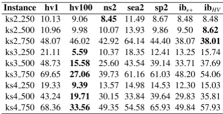
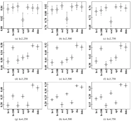
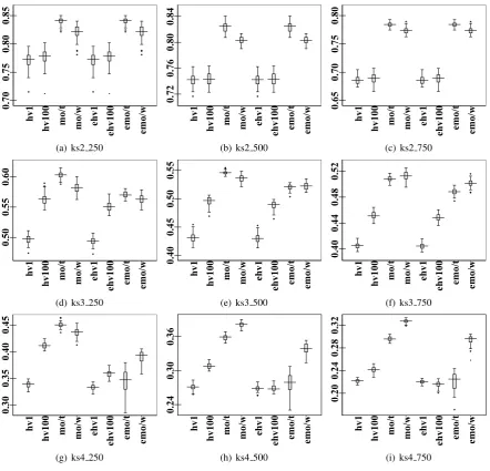
Regarding the hyper-volume metric,

Fig. 2,3,4,5 show that HVEA1.0 outperforms

or at least remains competitive to NSGA2, SEAMO2, SPEA2 on all 9 instances of the multiple 0/1 knapsack problem using all 4 different greedy repair methods. HVEA1.0 is

(12)

ib

h

v

ib

e

sp2

se

a

2

ns2

hv100

hv1

0.84

0.81

0.78

0.75

(a) ks2 250

ib

h

v

ib

e

sp2

se

a

2

ns2

hv100

hv1

0.80

0.76

0.72

(b) ks2 500

ib

h

v

ib

e

sp2

se

a

2

ns2

hv100

hv1

0.76

0.72

0.68

(c) ks2 750

ib

h

v

ib

e

sp2

se

a

2

ns2

hv100

hv1

0.55

0.50

0.45

(d) ks3 250

ib

h

v

ib

e

sp2

se

a

2

ns2

hv100

hv1

0.50

0.45

0.40

(e) ks3 500

ib

h

v

ib

e

sp2

se

a

2

ns2

hv100

hv1

0.50

0.45

0.40

(f) ks3 750

ib

h

v

ib

e

sp2

se

a

2

ns2

hv100

hv1

0.40

0.35

0.30

0.25

(g) ks4 250

ib

h

v

ib

e

sp2

se

a

2

ns2

hv100

hv1

0.36

0.32

0.28

0.24

(h) ks4 500

ib

h

v

ib

e

sp2

se

a

2

ns2

hv100

hv1

0.30

0.25

0.20

[image:12.595.78.519.97.509.2]

(i) ks4 750 Fig. 2: The percentage of hypervolume (permutation encoding).

Table 4: Running time in seconds (permutation)

ks2 250 7 6 6 4 48 50 50

ks2 500 14 14 14 9 97 96 91

ks2 750 27 28 26 21 165 160 144

ks3 250 14 18 11 7 103 103 158

ks3 500 28 38 23 15 179 175 242

ks3 750 46 66 39 32 272 264 368

ks4 250 24 52 18 11 184 183 354

ks4 500 44 114 36 22 294 286 545

ks4 750 68 204 56 48 415 407 771

in the lowest dimension space, the 2-knapsack

problems. HVEA1.0 only outperforms IBEA

(both IBEA+ and IBEAHV) for the 3-knapsack

problems. It looses its competitiveness to IBEA for 2,4-knapsack problems. IBEA+ tends to be the most effective MOEA to provide the coverage (hyper-volume) for the Pareto sets. It is also noticed that HVEA1.0performs much better than

HVEA0.01. The reason is that HVEA0.01 only

looks at a tiny neighbouring area to determine the crowdingof an individual whereas HVEA1.0

examines the objective space as the whole picture, i.e. every individuals contributing towards the crowding of an individual. Results on the generational and inverted generational distance

show more prominent evidence regarding

[image:12.595.81.278.579.676.2]

(13)

ib

h

v

ib

e

sp2

se

a

2

ns2

hv100

hv1

0.82

0.78

0.74

0.70

(a) ks2 250

ib

h

v

ib

e

sp2

se

a

2

ns2

hv100

hv1

0.78

0.75

0.72

0.69

(b) ks2 500

ib

h

v

ib

e

sp2

se

a

2

ns2

hv100

hv1

0.74

0.70

0.66

0.62

(c) ks2 750

ib

h

v

ib

e

sp2

se

a

2

ns2

hv100

hv1

0.55

0.50

0.45

(d) ks3 250

ib

h

v

ib

e

sp2

se

a

2

ns2

hv100

hv1

0.50

0.45

0.40

(e) ks3 500

ib

h

v

ib

e

sp2

se

a

2

ns2

hv100

hv1

0.45

0.40

0.35

(f) ks3 750

ib

h

v

ib

e

sp2

se

a

2

ns2

hv100

hv1

0.36

0.32

0.28

(g) ks4 250

ib

h

v

ib

e

sp2

se

a

2

ns2

hv100

hv1

0.30

0.25

0.20

(h) ks4 500

ib

h

v

ib

e

sp2

se

a

2

ns2

hv100

hv1

0.27

0.24

0.21

0.18

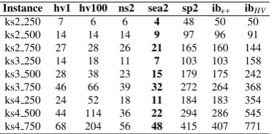
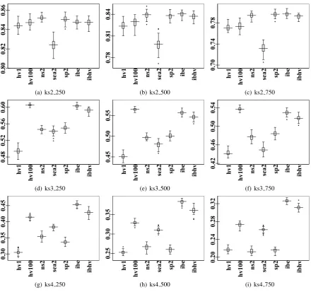
[image:13.595.78.519.99.507.2] [image:13.595.72.286.560.677.2]

(i) ks4 750 Fig. 3: The percentage of hypervolume (binary encoding).

Table 5: Generational distance (binary encoding)

ks2 250 3.91 3.78 4.17 6.16 4.09 6.95 6.99 ks2 500 11.42 11.03 13.39 15.10 13.78 17.66 18.07 ks2 750 26.86 27.10 32.87 33.91 31.67 29.48 30.05 ks3 250 8.45 13.95 22.16 8.62 14.18 10.06 9.77 ks3 500 20.83 34.04 50.69 21.39 32.63 24.47 22.82 ks3 750 35.71 55.08 74.63 40.78 52.56 38.58 35.84 ks4 250 14.18 33.23 38.58 13.91 27.10 15.37 14.99 ks4 500 31.13 75.38 96.31 30.97 66.35 32.20 28.85

ks4 750 52.80 119.03 150.58 52.89 106.08 53.40 44.81

Table 2,5,8,11 show the generational distance from non-dominated sets to the true Pareto front. Table 3,6,9,12 show the inverted generational

distance from the true Pareto front to non-dominated sets. Bold figures indicate the best results for each instance. Both sets of tables clearly indicate that HVEA1.0 provides better

diversity than HVEA0.01 whereas HVEA0.01

provides better convergence than HVEA1.0due to

the use of neighbouring area radius ω. On the performance regarding the generational distance

metric, HVEA0.01 outperforms NSGA2 and

(14)

that SEAMO2 is a steady-state algorithm which allows offspring to compete for recombination immediately within the current generation. It is not the case for the other population-based MOEAs. However it leads SEAMO2 to be one of the worst MOEAs to provide diversity for non-dominated sets. The inverted generational distance metric show that HVEA1.0 outperforms

other MOEAs in most cases of the 36 instance-repair method combination. HVEA1.0 is clearly

[image:14.595.307.529.107.399.2]

the best algorithm to provide diversity in high dimensional knapsack, 3,4-knapsack problems. There is no strong evidence for which algorithm is the best in the 2-knapsack problem.

Table 6: Inverted generational distance (binary encoding)

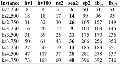
Table 7: Running time in seconds (binary)

ks2 250 8 8 7 6 50 51 51

ks2 500 18 18 17 14 99 96 95 ks2 750 31 32 30 26 165 157 149 ks3 250 16 20 12 9 104 103 145 ks3 500 31 39 25 21 175 170 236 ks3 750 50 61 43 36 266 256 350 ks4 250 27 50 19 14 185 183 351 ks4 500 47 107 37 28 281 278 537 ks4 750 73 168 60 48 396 392 746

[image:14.595.310.531.118.245.2]

The running time (in seconds) is summarised in table 4,7,10,??. SPEA2 and IBEA are the slowest algorithms due to the complexity in computation of fitness values (SPEA2) and indicator values (IBEA). SEAMO2, NSGA2, HVEA are much faster algorithms.

[image:14.595.310.525.246.393.2]

Taken all the above criteria into account, it is concluded that HVEA outperforms NSGA2, SEAMO2, and SPEA2 but remains competitive

Table 8: Generational distance (te binary encoding)

[image:14.595.74.286.336.446.2]

ks2 250 4.42 4.46 5.18 6.94 5.41 6.84 6.93 ks2 500 16.33 16.60 17.68 23.92 17.62 18.35 19.01 ks2 750 44.67 43.98 46.88 64.90 44.96 41.62 43.42 ks3 250 13.99 18.92 28.85 11.79 21.06 13.64 13.50 ks3 500 36.35 44.72 70.27 33.93 50.40 31.61 29.84 ks3 750 64.61 78.85 113.39 67.64 85.45 59.4756.29 ks4 250 22.82 40.94 47.44 16.53 37.85 17.53 17.29 ks4 500 51.52 89.40 114.67 40.71 89.75 43.0537.09 ks4 750 90.24 144.94 183.81 79.45 148.89 78.4867.98

Table 9: Inverted generational distance (te binary encoding)

Table 10: Running time in seconds (te binary)

ks2 250 13 13 12 10 54 55 60 ks2 500 31 31 30 26 112 109 117 ks2 750 58 58 56 51 192 182 198 ks3 250 22 28 18 16 109 110 150 ks3 500 51 61 46 40 195 191 256 ks3 750 93 109 86 76 310 301 392 ks4 250 36 66 30 24 195 194 367 ks4 500 75 143 66 57 307 308 565 ks4 750 134 256 129 108 462 461 810

to IBEA with much faster computational time than IBEA.

4.2. Comparison to MOEA/D

We compare HVEA against MOEA/D

separately from other MOEAs due to the setting and approach employed by MOEA/D. As discussed in Section 3.2.1, it is problematic

to alter the population size N in MOEA/D

to that population size S suggested for the

multiple 0/1 knapsack problem. Furthermore,

MOEA/D stores all non-dominated solutions

[image:14.595.315.521.431.544.2] [image:14.595.76.282.495.606.2]

(15)

ib

h

v

ib

e

sp2

se

a

2

ns2

hv100

hv1

0.84

0.82

0.80

(a) ks2 250

ib

h

v

ib

e

sp2

se

a

2

ns2

hv100

hv1

0.82

0.80

0.78

0.76

(b) ks2 500

ib

h

v

ib

e

sp2

se

a

2

ns2

hv100

hv1

0.76

0.72

0.68

(c) ks2 750

ib

h

v

ib

e

sp2

se

a

2

ns2

hv100

hv1

0.58

0.54

0.50

0.46

(d) ks3 250

ib

h

v

ib

e

sp2

se

a

2

ns2

hv100

hv1

0.52

0.48

0.44

0.40

(e) ks3 500

ib

h

v

ib

e

sp2

se

a

2

ns2

hv100

hv1

0.46

0.42

0.38

(f) ks3 750

ib

h

v

ib

e

sp2

se

a

2

ns2

hv100

hv1

0.40

0.35

0.30

(g) ks4 250

ib

h

v

ib

e

sp2

se

a

2

ns2

hv100

hv1

0.35

0.30

0.25

0.20

(h) ks4 500

ib

h

v

ib

e

sp2

se

a

2

ns2

hv100

hv1

0.25

0.20

0.15

[image:15.595.77.519.97.509.2]

(i) ks4 750 Fig. 4: The percentage of hypervolume (te binary encoding).

then reported as the final result. Therefore, it is suggested to adapt HVEA to the setting similar to MOEA/D included the population size and an external archive for non-dominated solutions found so far. Experimental results, including figures and tables, are presented in a similar

format as in Section 4.1. MOEA/D employed

Tchebycheff and weight sum approach for the

fitness calculation are abbreviated as “mo/t” and “mo/w”. The extracted population, the truncated external population, is also reported so that the size of the extracted population does not exceed

the suggested population size S. NSGA2’s

truncation approach is used here. Fig. 6,7,8,9

[image:15.595.319.515.584.706.2]

present extracted populations using prefix “e”.

Table 11: Generational distance (ws binary encoding)

ks2 250 2.02 1.96 2.24 3.89 2.07 2.91 2.92 ks2 500 6.13 6.07 6.70 10.80 6.74 8.07 8.59 ks2 750 16.53 16.38 18.42 27.96 17.26 17.40 17.62 ks3 250 9.52 12.17 20.82 7.26 14.23 7.87 7.46 ks3 500 20.87 27.25 47.72 16.50 31.60 16.88 15.90

ks3 750 30.72 42.91 67.05 25.88 45.73 27.35 24.99

ks4 250 17.06 29.66 35.52 12.52 27.13 13.59 13.35 ks4 500 33.58 60.66 82.87 25.34 59.50 27.40 23.68

ks4 750 54.58 97.91 131.27 42.68 96.22 44.91 38.29

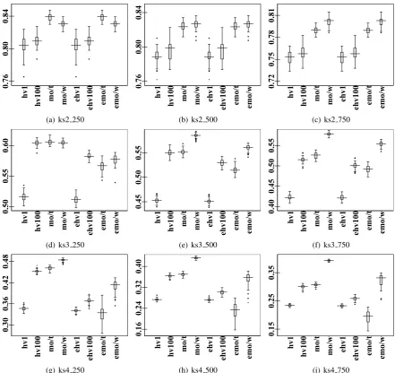
MOEA/D outperforms HVEA in most cases

(16)

ib

h

v

ib

e

sp2

se

a

2

ns2

hv100

hv1

0.86

0.84

0.82

0.80

(a) ks2 250

ib

h

v

ib

e

sp2

se

a

2

ns2

hv100

hv1

0.84

0.81

0.78

(b) ks2 500

ib

h

v

ib

e

sp2

se

a

2

ns2

hv100

hv1

0.78

0.74

0.70

(c) ks2 750

ib

h

v

ib

e

sp2

se

a

2

ns2

hv100

hv1

0.60

0.56

0.52

0.48

(d) ks3 250

ib

h

v

ib

e

sp2

se

a

2

ns2

hv100

hv1

0.55

0.50

0.45

(e) ks3 500

ib

h

v

ib

e

sp2

se

a

2

ns2

hv100

hv1

0.54

0.50

0.46

0.42

(f) ks3 750

ib

h

v

ib

e

sp2

se

a

2

ns2

hv100

hv1

0.45

0.40

0.35

0.30

(g) ks4 250

ib

h

v

ib

e

sp2

se

a

2

ns2

hv100

hv1

0.35

0.30

0.25

(h) ks4 500

ib

h

v

ib

e

sp2

se

a

2

ns2

hv100

hv1

0.32

0.28

0.24

0.20

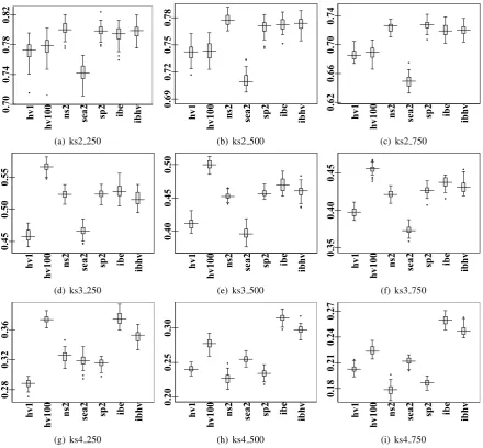
[image:16.595.78.519.97.510.2]

(i) ks4 750 Fig. 5: The percentage of hypervolume (ws binary encoding).

on the hyper-volume metric and the inverted generational distance metric. The convergence of MOEA/D is only better than that of HVEA in the linear scalarising greedy repair method. However the running time of MOEA/D is significantly higher than that of HVEA. In the other 2 repair methods, HVEA0.01 outperforms

MOEA/D regarding the generational distance metric. Under a restriction of the size of the population, where the truncation is applied to the external population, HVEA is able to compete to MOEA/D. However HVEA is much faster than MOEA/D. The running time (in seconds) is reported in Table 18, 15, 21, 24.

Table 12: Inverted generational distance (ws binary encoding)

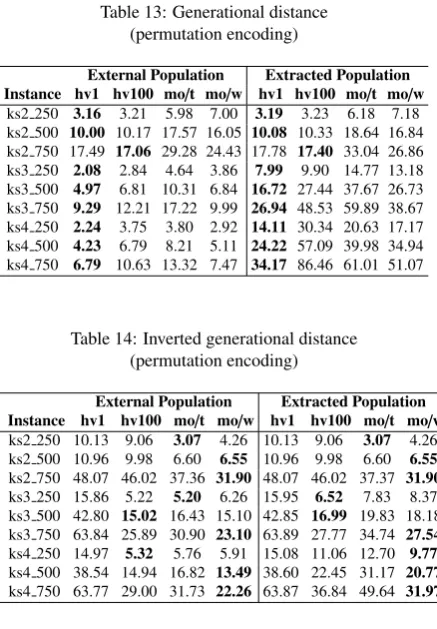
ks2 250 3.80 3.40 2.70 4.90 3.05 3.14 3.34 ks2 500 7.02 6.62 4.97 9.05 5.27 4.53 4.78 ks2 750 41.14 40.31 28.86 52.55 27.86 26.11 27.82 ks3 250 16.83 4.78 9.71 17.31 8.93 9.06 11.05 ks3 500 40.25 13.21 22.43 40.48 24.74 23.92 27.69 ks3 750 56.43 23.72 35.38 59.39 37.02 36.85 41.70 ks4 250 16.08 7.75 11.47 14.33 11.35 9.17 11.85 ks4 500 37.35 18.10 27.27 32.41 28.35 22.44 27.55 ks4 750 58.56 31.92 46.15 52.21 47.00 38.13 45.26 4.3. Further Discussion

[image:16.595.312.522.576.693.2]

(17)

e m o /w e m o /t e h v 1 0 0 e h v 1 m o /w m o /t hv100 hv1 0.84 0.80 0.76

(a) ks2 250

(b) ks2 500

e m o /w e m o /t e h v 1 0 0 e h v 1 m o /w m o /t hv100 hv1 0.81 0.78 0.75 0.72

(c) ks2 750

(d) ks3 250

(e) ks3 500

(f) ks3 750

(g) ks4 250

(h) ks4 500

[image:17.595.76.518.98.514.2]

(i) ks4 750 Fig. 6: The percentage of hypervolume (permutation encoding).

µ is set to 0.01, which is not only bounded to the multiple 0/1 knapsack problem, could be used for other multi-objective optimisation problems. It is suggested that this parameter µ is fixed to 0.01 rather than tunable. The more important parameter in HVEA is ω, theneighbouring area radius, which is in the range [0,1]. Section 4.1 shows a significant difference in performance between HVEA0.01 and HVEA1.0. HVEA1.0

gives a much better performance regarding the hyper-volume metric and the diversity of the

non-dominated set. However HVEA0.01 is better

in convergence than HVEA1.0. One could

tune ω to obtain desirable requirement. For

example, ω could be set to 1.0 for theoretical

problems such as the multiple 0/1 knapsack

problem to obtain non-dominated set with better diversity (generational distance metric) and better coverage (hyper-volume metric). However, for real-world applications, where running time is

expensive, ω = 0.01 could be deployed.

Furthermore, in real-world applications, extreme solutions are likely less of interest whereas better convergence, which could strike a good balance

amongst objectives, is more important. We

(18)

but the performance of HVEA degrades quite significantly. Therefore, it is suggested to use

[image:18.595.310.523.98.546.2]

ω = 1.0 for better diversity and better coverage and 0.01 ≤ ω ≤ 0.05 for better convergence and faster computational time.

Table 13: Generational distance (permutation encoding)

External Population Extracted Population Instance hv1 hv100 mo/t mo/w hv1 hv100 mo/t mo/w

[image:18.595.71.290.182.497.2]

ks2 250 3.16 3.21 5.98 7.00 3.19 3.23 6.18 7.18 ks2 500 10.00 10.17 17.57 16.05 10.08 10.33 18.64 16.84 ks2 750 17.49 17.06 29.28 24.43 17.78 17.40 33.04 26.86 ks3 250 2.08 2.84 4.64 3.86 7.99 9.90 14.77 13.18 ks3 500 4.97 6.81 10.31 6.84 16.72 27.44 37.67 26.73 ks3 750 9.29 12.21 17.22 9.99 26.94 48.53 59.89 38.67 ks4 250 2.24 3.75 3.80 2.92 14.11 30.34 20.63 17.17 ks4 500 4.23 6.79 8.21 5.11 24.22 57.09 39.98 34.94 ks4 750 6.79 10.63 13.32 7.47 34.17 86.46 61.01 51.07

Table 14: Inverted generational distance (permutation encoding)

External Population Extracted Population

Instance hv1 hv100 mo/t mo/w hv1 hv100 mo/t mo/w

ks2 250 10.13 9.06 3.07 4.26 10.13 9.06 3.07 4.26 ks2 500 10.96 9.98 6.60 6.55 10.96 9.98 6.60 6.55

ks2 750 48.07 46.02 37.36 31.90 48.07 46.02 37.37 31.90

ks3 250 15.86 5.22 5.20 6.26 15.95 6.52 7.83 8.37 ks3 500 42.80 15.02 16.43 15.10 42.85 16.99 19.83 18.18 ks3 750 63.84 25.89 30.90 23.10 63.89 27.77 34.74 27.54

ks4 250 14.97 5.32 5.76 5.91 15.08 11.06 12.70 9.77

ks4 500 38.54 14.94 16.82 13.49 38.60 22.45 31.17 20.77

ks4 750 63.77 29.00 31.73 22.26 63.87 36.84 49.64 31.97

We further examine the performance of HVEA against other MOEAs using a fixed running time, although this approach is not widely adopted due to its low reliability. The running time (in seconds), reported in Table 25, is deduced from the minimum running time of all MOEAs on each knapsack instances over 2000 generations. The running time for the linear scalarising greedy repair method proposed by Jaszkiewicz [13] is twice as much as the ones proposed by Mumford [12] and Zitzler and Thiele [11].

Under the time restriction, HVEA outperforms

NSGA2, SPEA2, IBEA+ and IBEAHV. HVEA

only outperforms SEAMO2 on 2,3-knapsack problems. SEAMO2 is slightly better than HVEA on 4-knapsack problems. It is suggested that due to the steady-state approach and the simple Pareto dominance, SEAMO2 is able to perform more

Table 15: Running time in seconds (permutation)

Instance hv1 hv100 mo/t mo/w

ks2 250 4 5 3 4

ks2 500 8 9 8 9

ks2 750 15 16 17 19

ks3 250 16 26 40 38

ks3 500 29 84 118 133 ks3 750 46 177 172 181 ks4 250 47 156 357 315 ks4 500 112 602 1025 972 ks4 750 163 870 1784 1807

Table 16: Generational distance (binary encoding)

[image:18.595.71.286.203.325.2]

ks2 250 3.91 3.78 4.47 7.28 3.91 3.78 4.54 7.29 ks2 500 11.42 11.03 15.53 17.39 11.42 11.03 15.53 17.39 ks2 750 26.86 27.10 34.07 34.88 26.86 27.10 34.07 34.88 ks3 250 3.26 4.08 4.77 4.57 10.18 12.28 14.33 14.01 ks3 500 10.67 10.69 12.18 10.15 24.41 31.16 37.44 32.18 ks3 750 22.54 22.11 23.62 19.32 38.93 53.36 64.60 52.75 ks4 250 3.26 4.46 4.08 3.63 16.27 26.40 21.17 19.24 ks4 500 9.37 11.80 10.06 8.09 35.47 69.12 49.77 44.30 ks4 750 18.56 20.13 16.93 12.85 57.80 114.62 80.97 71.23

Table 17: Inverted generational distance (binary encoding)

ks2 250 14.55 13.88 2.78 5.35 14.55 13.88 2.79 5.35 ks2 500 17.97 17.91 5.36 7.37 17.97 17.91 5.36 7.37 ks2 750 81.69 81.09 33.08 35.57 81.69 81.09 33.08 35.57 ks3 250 16.31 8.36 5.22 8.37 16.36 8.93 7.41 9.67 ks3 500 41.47 25.90 17.05 24.17 41.50 26.38 20.07 25.59 ks3 750 61.05 42.30 30.87 34.95 61.08 42.67 33.83 36.71 ks4 250 14.87 6.95 6.10 8.84 14.97 10.12 11.59 10.91 ks4 500 34.46 19.55 17.22 19.04 34.53 24.15 24.86 22.39

[image:18.595.71.296.377.485.2]

ks4 750 56.85 36.89 32.02 32.62 56.92 41.66 43.02 36.28

Table 18: Running time in seconds (binary)

Instance hv1 hv100 mo/t mo/w

ks2 250 8 8 5 5

ks2 500 18 19 13 13

ks2 750 32 33 25 25

ks3 250 25 35 18 18

ks3 500 39 56 39 40

ks3 750 56 74 59 57

ks4 250 55 139 113 87

ks4 500 82 285 359 342