Small angle neutron scattering studies of magnetic recording media

SMALL ANGLE NEUTRON SCATTERING STUDIES OF MAGNETIC RECORDING MEDIA

Matthew P. Wismayer

A Thesis Submitted for the Degree of PhD at the

University of St. Andrews

2008

Full metadata for this item is available in the St Andrews Digital Research Repository

at:

https://research-repository.st-andrews.ac.uk/

Please use this identifier to cite or link to this item:

http://hdl.handle.net/10023/471

This item is protected by original copyright

This item is licensed under a

Small Angle Neutron Scattering Studies of

Magnetic Recording Media

By

Matthew P. Wismayer

B.Sc.Honours (York University) 1998

M.Sc. (Carleton University) 2001

University

of

St Andrews

ii

Declaration

I Matthew Wismayer hereby certify that this thesis is approximately 50,000 words in length, has been written by me, that it is the record of work carried out by me and that it has not been submitted in any previous application for a higher degree

Date………signature of candidate………

I was admitted as a research student in September 2003 and as a candidate for the degree of Doctor of Philosophy in September 2004; the higher study for which this is a record was carried out in the University of St. Andrews between 2003-2007.

Date………signature of candidate………

I hereby certify that the candidate has fulfilled the conditions of the Resolution and Regulations appropriate for the degree of Doctor of Philosophy in the University of St. Andrews and that the candidate is qualified to submit this thesis in application for that

degree.

Date………signature of supervisor………

In submitting this thesis to the University of St.Andrews I understand that I am giving permission for it to be made available for use in accordance with the regulations of the University Library for the time being in force, subject to any copyright vested in the

work not being affected thereby. I also understand that the title and abstract will be published, and that a copy of the work may be made and supplied to any bona fide library or research worker.

iii

Acknowledgements

In the past four years, the following people have made a significant contribution to this thesis project. I would like to thank my supervisor Professor Stephen Lee, who has assisted with the project’s experimental and theoretical topics. I would like to acknowledge Dr. Tom Thomson of Hitachi San Jose Research Center, who provided the project with the longitudinal and perpendicular media samples. I would like to acknowledge Dr. Feodor Ogrin of Exeter University, who has provided guidance for the micromagnetic simulations of longitudinal recording media. At the University of St. Andrews, I would like to thank the people of Stephen Lee’s condensed matter physics group Stephen Lister, David Heron, Alan Drew and Ujjual Divakar.

Acknowledgements go to Dr. Charles Dewhust of D22, ILL Grenoble France, who provided guidance and analysis during the SANS experiments. In addition I would like to thank Dr. J. Kohlbrecher of SINQ, PSI Switzerland, who has assisted on the experimental and theoretical aspects of polarised SANS. Further thanks go out to the researchers Dr. Y. Peng and Dr. T.H. Shen at the University of Salford, who provided this project with the cobalt nanowire and sample holder.

iv

Abstract

In the beginning of the twenty-first century, educational and commercial institutions have driven the demand for cheap and efficient data storage. The storage medium known as magnetic recording media has remained the mainstay for most computer systems due to its large storage capacity per dollar. With the recording media’s ever-increasing storage density has come reductions in the magnetic grain size per bit. At the recording bit’s density threshold, the magnetic grains become more susceptible to thermal activation, which can render the storage medium unusable. An accurate characterisation of the recording layer’s sub-granular structure is essential for understanding the magnetic and thermal mechanisms of high-density recording media. Small-Angle Neutron Scattering (SANS) studies have been performed to investigate the magnetic and physical properties of longitudinal and perpendicular recording grains.

The SANS studies of longitudinal magnetic recording media have probed the recording layer’s magnetic grain size at a sub-nanometer resolution. In conjunction with these studies, SQUID magnetometry was used to characterise the recording grain’s bulk magnetism. Measurements showed that the recording grain was composed of a ferromagnetic hard core (Co-enriched) and a weakly magnetic shell (Cr-enriched).

These results provided important information on the grain’s magnetic anisotropy, which determines the recording media’s magnetic stability. The polarised SANS studies were used to characterise the recording layer’s physical granular structure. It was shown that the physical grain size was comparable to its magnetic counterpart. These physical

measurements provided insight into the recording grain’s chemical composition.

v

Contents

Acknowledgements…..……….………iii

Abstract……….………iv

Contents………...……..………v

List of Figures………...………ix

List of Tables………....………...…xxiv

Abbreviations……..…….……..………xxv

List of Symbols and Constants..….………..…....xxvi

Chapter 1 Introduction to Magnetic Recording Media

1.1 Historical Review.…………...……….……... 2

1.2 Previous Work.………….…………..……….… 12

1.2.1 Longitudinalmedia..…...……..……….……….………. 13

1.2.2 Perpendicular media…...…………...……… 18

1.2.3Summary..…….………...…………....……… 19

Chapter 2 Theoretical Background

2.1Magnetism…..…...………. 21

2.1.1 Diamagnetism.…....……….... 24

2.1.2 Paramagnetism…...….………... 25

2.2 Spontaneous Magnetism….………... 27

2.2.1 Ferromagnetism...…..………. 28

2.2.2 The Curie Phase Transition.……....…..……..……… 30

2.2.3 Domain Theory…………..……...…....………...…..…………. 33

2.2.3.1 DipolarField.……….. 33

2.2.3.2 Magnetic Anisotropy...………. 34

2.2.3.3 Magnetic Hysteresis……….……….. 36

2.3 Neutron Scattering………...………….……… 38

2.3.1 Elastic Nuclear Scattering..……….…………...………. 40

Contents vi

2.4 Polarised Neutron Scattering…..……… 44

2.4.1 Nuclear-Magnetic Interference Scattering….……… 45

2.5 Amorphous Scattering……….…………...……… 46

2.5.1 Multi-Bodied Scattering.……….…...………..….. 48

Chapter 3 Experimental Techniques and Instrumentation

3.1 Small Angle Neutron Scattering...………...………... 53

3.1.1 SANS Instrumentation....………….………... 54

3.1.2 SANS Geometry…...….……….… 61

3.2 Magnetometry....…….………..….………. 62

3.2.1 SQUID…….……….……….………. 62

3.2.2 VSM and MOKE....………...……….… 64

Chapter 4 Longitudinal Magnetic Recording Media

4.1Introduction....………..……... 67

4.2 The Recording Media Sample....………. 69

4.2.1 Sample Fabrication...……… 71

4.2.2 SeedLayer...………...………. 73

4.2.3 Recording Layer...……….. 74

4.3 Bulk Magnetisation..….…………...………... 78

4.3.1Measurements.……….... 78

4.3.2 Results and Discussion-AX1821.………..………. 79

4.3.3 Results and Discussion-AX1646...…….……….. 82

4.3.4 Results and Discussion-AX341….……...……….. 85

4.3.5 Summary.……...….……….………... 89

4.4 Unpolarsied SANS…………...………... 90

4.4.1 Scattering Model....….……….... 90

4.4.2Instrumentation..…….……… 95

4.4.3Measurements..…..….……… 98

4.4.4 Results and Discussion-AX1821..….……….... 104

4.4.5 Results and Discussion-AX1646..………. 109

4.4.6 Results and Discussion-AX341..………...……… 128

Contents vii

4.5 Polarised SANS.………. 137

4.5.1 Instrumentation.………. 138

4.5.2 Measurements.….……….. 140

4.5.3 Results and Discussion..….……….... 143

4.5.4 Summary……….…….……….. 152

4.6 Conclusion……….………...………. 152

Chapter 5 Perpendicular Magnetic Recording Media

5.1 Introduction...….…………...………. 155

5.2The Recording Media Sample...……….……….. 157

5.2.1 Recording Layer..………... 158

5.2.2 Seed Layer...………... 159

5.2.3 Soft Magnetic Underlayer...………... 161

5.3 Bulk Magnetisation.……...…...………. 162

5.3.1 Results and Discussion....……….. 163

5.4 Unpolarised SANS....…….……….... 166

5.4.1 Scattering Model...……….……….. 166

5.4.2 Instrumentation...….……….………. 168

5.4.3 Measurements…….……….……….. 169

5.4.4 Results and Discussion…..……….... 172

5.4.5 Summary………...………...……….. 186

5.5Polarised SANS.………. 186

5.5.1 Instrumentation……….………. 187

5.5.2 Measurements….………….……….. 188

5.5.3 Results and Discussion...……….... 190

5.5.4 Summary……….……....….……….. 202

5.6 Conclusion...….……....……….. 203

Chapter 6 Ferromagnetic Nanowires

6.1Introduction.……….……….………..………... 205

6.2 Physical Microstructure.…..………... 206

Contents viii

6.4 Unpolarised SANS………...……….... 209

6.4.1 Scattering Model.….……….. 209

6.4.2 Instrumentation..…...………..………... 211

6.4.3 Measurements.…….………..……….... 212

6.4.4 Results and Discussion...…...………...…..…… 213

6.4.5 Summary.………….…...………..……... 223

6.5 Conclusion….…...….…………..……….. 223

Chapter 7 Magnetic SANS Simulations

7.1 Introduction..…...…...……… 225

7.2 Micromagnetic Method..….………... 226

7.2.1 OOMMF Simulations.…..……….. 228

7.2.2 MagneticScattering Theory.…..…..……….. 231

7.3 Ferromagnetic Nanowires.…....….……….………... 232

7.3.1 Simulations..…....………...….…..………. 232

7.3.2 Results and Discussions.…………..……..……… 234

7.3.3 Summary.……….………….…....….……..……….. 237

7.4 Longitudinal Magnetic Recording Media..….….……….……. 237

7.4.1 Simulations....………....………...………. 238

7.4.2 Results and Discussion...……….…..……… 240

7.4.3 Summary....…………...……...…....……….. 246

7.5Conclusion..………….…..………...……….. 247

Chapter 8 Appendices

8.1 The Form Factor……...………....……….………. 249

8.1.1 Sphere..……….. 249

8.1.2Cylinder.………. 250

8.2 The Structure Factor..………...………. 251

8.3 Publications...………….……...……….………. 253

ix

List of Figures

1.1 The simplified schematic shows the working components of the first telegraphone. The metallic wire is coated in a ferromagnetic oxide, which acts as the device’s recording medium [2]…………...………....2

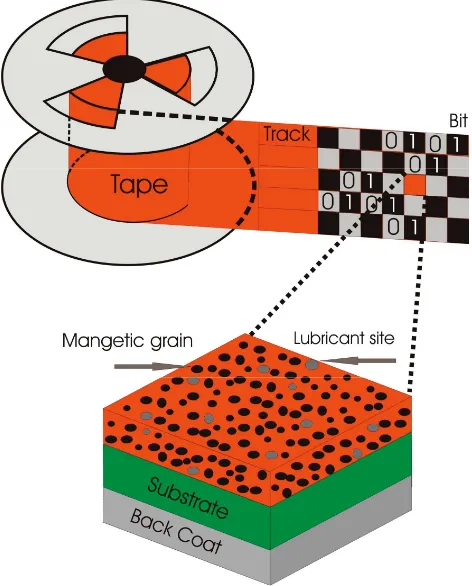
1.2 The cross-section of longitudinal magnetic recording tape. The magnetic medium is composed of a ferromagnetic oxide grown onto thin a plastic substrate. The recording grains form the recording bit, which lies along the tape

track [6]………...3

1.3 This schematic outlines the advantages from converting the storage medium to the magnetic tape………..……….4

1.4 The IBM 350 hard disk drive consists of a drum of thin magnetic discs. The cross-section shows the first generation longitudinal magnetic media [9,10]…..5

1.5 The schematic of a conventional longitudinal magnetic hard disk drive. The medium’s cross-section shows the CoCrPtTa recording layer grown onto the Cr-alloy seed layer and NiP underlayer [12]………….……..…………..………….7

1.6 The recording grain’s internal energies UK1, UK2 and UK3 as a function of magnetisation angle. The energy barrier is enlarged by increasing the grain’s magneto-crystalline anisotropy energy density where K3>K2>K1….…..……….7

1.7 The cross-section of Anti-Ferromagnetic Coupled Media (AFC). The AFC geometry is the similar to the longitudinal media except for the non-magnetic Ru spacer between the recording layers [15]………..8

1.8 The schematic of perpendicular magnetic recording media. The cross-section shows the CoCtPt-SiO2 recording layer grown onto a Ru seed layer and CoFe

underlayer [17]………10

1.9 The demagnetisation field of the longitudinal and perpendicular bit for (a) thin film, (b) low density and (c) high density [18]………10

1.10 The chart follows the history of the disk drive by plotting the areal density as a function of production year.…..………..11

1.11 The EEL-TEM measurements of CoCr15Ta4 (a) zero-Loss, (b) Cr core-loss and (c) Co core-loss [21]..…..………...13

List of Figures x

1.13 The SANS foreground (H=6.0 kOe) and background (H=0) measurements for (a) sample Cy. The magnetic scattering intensity is plotted for the samples (b) Cy, (c) To and (d) So. The scattering data is fitted with a cylindrical form factor averaged over a log-normal distribution of cluster sizes [25]……….……15

1.14 The log-distribution plot for samples Cy(), To(--),So(- . -). The arrow marks the position of the average cluster size. The inset compares the magnetic cluster size to the physical grain size [25]………...16

1.15 The small-angle x-ray measurements for longitudinal recording media. In (a) the scattering intensity as a function of q is plotted for the Co and Cr excitation edge where in (b) the spectrum is plotted for the peak positions of q=0.013 Å-1 and q=0.057 Å-1

[26]………....17

1.16 The magnetic and nuclear cross-sections for (a) bulk and (b) thin film Co-Cr alloy samples. The bulk SANS data is fitted using the Porod function, while the thin film scattering is modelled using the spherical core-shell form factor [27].18

1.17 Soft x-ray resonant scattering for perpendicular orientated CoCrPt grains shown in (a). The scattering intensity (b) is extracted for the Co and Cr edges [28]…19

2.1 The Ampere model for classical magnetism. The total dipole moment, µt is the superposition of smaller current loops within the magnetic material…………..21

2.2 The quantum paramagnetic moment plotted using the Brillouin function B(y)=(2J+1)/2Jcoth((2J+1)/2Jy)-1/2Jcoth(2J*y) for J=1/2, 3./2, 2, ∞…………26 2.3 The magnetic susceptibility as a function of temperature. The metals (a) Cu and Au show a diamagnetic response while the substances (b) Al and NiAl are characteristic of a Curie paramagnet [35,36]………...26

2.4 The spin up/down density of states of a non-magnetic metal. The substance exhibits paramagnetism when an applied magnetic field causes an energy shift between the spin bands [32]………29

2.5 The spin up/down density of states for a band ferromagnet. At zero applied field, the shift between spin bands is due to the metal’s internal molecular field

w

[32]………..……….29

2.6 The mechanism for the Weiss theory of ferromagnetism. The centre moment is aligned by a molecular field (green arrows) generated by its nearest neighbour moments………...30

2.7 Graphical solutions to the Brillouin (intersections) function at the magnetic states T<<TC, T<TC, T=TC and T>TC………..32

List of Figures xi

2.9 Formation of the (a) single domain, (b) anti-parallel domain, (c) multiple domains and (d) domain flux closure where the sample’s net magnetisation goes

to zero………..33

2.10 The hcp crystal structure for the ferromagnetic rare earth Tb. The crystal easy axis is directed along the b-axis. The right plot shows the Tb magnetisation measured along the c and b axes [36]….………35

2.11 Illustrations of magnetic shape anisotropy for the (a) thin film and (b) an ensemble of infinitely long cylindrical objects. The atomic moments shown in the rectangular box, align along the easy axis of magnetisation that turns out to be the spatial dimension of largest extent………...………35

2.12 The magnetic hysteresis loop for the typical ferromagnet. The virgin state at M=0 is brought to saturation Ms. At zero the magnetisation remains finite defined by the remanent magnetisation Mr. The zero magnetisation states are defined at the coercive field Hc……….………..37

2.13 The magnetic hysteresis loop ranging from (a) hard to (d) soft ferromagnet…..37

2.14 The incident neutron plane wavescattering off a spherical target [43]...……...38

2.15 The neutron and x-ray scattering amplitudes plotted as a function of atomic weight. The solid linear plots represent the x-ray scattering amplitude while the dashed line relates to the nuclear scattering component [44]…..………39

2.16 The conventional scattering experiment used to derive the nuclear scattering cross-section.………40

2.17 Vector plot of the interaction magnetisation field M⊥⊥⊥⊥(q)=qˆ×(M(q)×qˆ)…...43 2.18 Spatial representations of the crystal, liquid and gas phase. For each phase state, the elastic scattering intensity is plotted in reciprocal space [44,45]…..………47

2.19 Model for an ensemble of polydisperse scattering potentials U(xi)………48

2.20 The form factors intensity plotted for the spherical and cylindrical object. The form factor intensities are compared with the Porod scattering function Aq-4…49

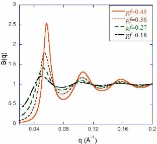
2.21 Monodisperse liquid structure factor S(q) calculated using the Percus-Yevick integral method. The structure factor is investigated by varying the packing fraction pf. The S(q) exhibits crystal like scattering for large pf value. Scattering from secondary peaks becomes weak for pf <0.27 [59]……….51

2.22 Polydisperse liquid structure factor S(q) calculated using the Percus-Yevick integral method. The S(q) distribution of hard spheres is investigated for a pf=0.36. At a large size distribution, the pair correlations reduce to unity…....51

List of Figures xii

3.2 The schematic of the conventional SANS instrument. The device is set-up to measure nuclear and magnetic structures for the energy scale of 10-2 eV……...55

3.3 The reactor guide tube that transports the neutrons to the moderator [38]……..55

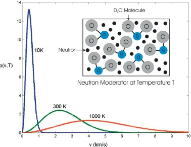
3.4 The Maxwell-Boltzmann distribution for thermal neutron velocities. The figure inset shows the thermalisation of neutrons within the D2O moderator………...56

3.5 The schematic of a Dornier velocity selector. In setup (a) the incident neutron beam, with an average velocity Vin=Vave, is chopped by the stationary velocity selector. In setup (b) the incident neutrons pass through the rotating selector with velocity Vout=V′ave………57 3.6 The polarisation of the incident neutron beam through total reflection from the

Fe/Si multi-layer………..58

3.7 The side and top view of the SANS collimator. The guide section G0 remains fixed. To change the collimation length the guide Gi and collimation Ci sections for i=1,2,3 rotate in and out of the neutron beam………59

3.8 The schematic of 3He position sensitive detector. The detector consists of a reaction chamber that contains the 3He atoms and the detector electronics. The scattering intensity is converted to a pixelated map of q space………...60

3.9 The scattering geometry for the SANS target and two-dimensional detector. The circular inset depicts the neutron scattering event within the Bragg plane…….61

3.10 The SQUID junction threaded with an external flux. The voltage across the SQUID osciilates as a function of external flux……….63

3.11 A simplified schematic of the SQUID chip, cryomagnet and sample mount…..63

3.12 The simplified schematics of the (a) VSM and (b) MOKE instruments...……..65

3.13 The diagram (a) shows the MOKE reflection for the longitudinal, polar and transverse magnetisation. The Kerr rotation is observed in the (b) S′-P′ plane where ±θP defines the rotation angle of the analyser………..………65 4.1 The log-normal distribution for an ensemble of recording grains with the standard deviation fractions of (a) 0.6, (b) 0.3 and (c) 0.1……….68

4.2 The composition and dimensions of the CoCrPtB LMRM sample……….70

4.3 The cross-section for the conventional longitudinal magnetic recording film…72

List of Figures xiii

4.5 The crystallattice matching for Co(101)/C(110) and Co(100)/Cr(112)……….73

4.6 The CoCrPt longitudinal recording layer’s (a) granular ensemble, (b) single grain and the (c) crystalline lattice………..…74

4.7 The schematic of a bi-crystal longitudinal recording layer. The bi-crystal grains form orthogonal moment pairs which are coupled via exchange forces….……75

4.8 The saturation magnetisation of the CoCrPt alloy as a function of the atomic percentage of Cr [83]..……….…76

4.9 The magneto-crystalline anisotropy field HK of the compound CoCrPtB as a function of the atomic percentage of Pt [84]………...77

4.10 The AX1821 in-plane magnetic hysteresis at the temperature of 5 K...……..…80

4.11 The AX1821 in-plane magnetic hysteresis at the temperature of 300 K.………80

4.12 The AX1821 magnetisation at the temperatures of (a) 5 K and (b)300 K...…81

4.13 The AX1646 in-plane magnetic hysteresis measurements of the total moment, background and recording layer components at the temperature of 5K…….…83

4.14 The AX1646 in-plane magnetic hysteresis measurements of the total moment, background and recording layer components atthe temperature of 300 K....…83

4.15 The AX1646 magnetisation at the temperatures of (a) 5K and (b) 300K……..84

4.16 The AX341 in-plane magnetic hysteresis measurement of the total moment, background and recording layer at the temperatures of(a) 5 K and 300 K...….86

4.17 The AX341 magnetisation at the temperatures of (a) 5 K and (b) 300 K…..….86

4.18 The saturation magnetisation of the LMRM samples AX1646 and AX341 plotted as a function of temperature….………...……….87

4.19 The coercive field of AX1646 and AX341 as a function of temperature...…….88

4.20 The TEM image of the conventional LMRM film [88]. The granular structure is modelled using cylindrical objects embedded in the grain boundary matrix…..92

4.21 The magnetic recording grain is represented as a series of scattering surfaces. The effect of magnetic softening occurs at the grain’s surface where S1→S3 represents the transition from cylindrical to spherical grain. The scattering potential V0 is plotted as a function of the grain’s radius R………93

List of Figures xiv

4.23 Snapshots of the D11 SANS instrument. The first image (a) shows an overview of the SANS tube which houses the 3He position sensitive detector. The tube extends to the far end of the instrument hall………...96

4.24 The schematic of the aluminium sample holder. The 26 samples are fastened to an aluminium ring located at the centre of the holder. The Cd mask is fabricated with a 1.4 cm aperture that allows the incident beam to illuminate the sample..97

4.25 The transmissionmeasurement at the detector distance of 1.5m...………99

4.26 The incident neutron beam flux as a function of collimator distance.…………99

4.27 The magnetisation map within the recording layer where <M> defines the sample’s remanent magnetisation. The anisotropic magnetic diffraction plot is illustrated for each remanent state…………...………..100

4.28 The modelled diffraction patterns for the isotropic background scattering IB(q) and the foreground scattering intensity IF(q) where the magnetisation unit vector m is defined along the qx axis. The nuclear and magnetic components are represented bythe Porod scattering intensity………...101

4.29 The simulated 2D and 3D magnetic difference plots resulting from the superposition of anisotropic and isotropic scattering components………102

4.30 The simulated difference plot for an in-plane moment along the qx and qy axes. The ANCOS2 function fits the difference plot over an annular ring of radius qi and width ∆qi. The amplitude Ib, offset Ia and phase shift δc are defined on the azimuthal scattering intensity plot………103

4.31 The AX1821 1.0T foreground IF(q) and background IB(q) measurements at the sample-detector distance of 1.50m. The subtraction results in the magnetic difference expressed in cross-section units.………..104

4.32 The AX1821 1.0T magnetic difference plot measured at the sample-detector distance of 1.5 m. The azimuthal scattering intensity is calculated over the q range 0.04Å-1 <q1.5m<0.30 Å-1. The orientation dependence is expressed by sin2α. The azimuthal scattering intensity is fitted by the function Ia+Ibcos2(θ+δc) where θ=900-α...………105 4.33 The AX1821 1.0T foreground measurement and the anisotropic magnetic scattering intensity...………..106

4.34 The AX1821 1.0T anisotopic magnetic scattering intensity fitted to the Porod scattering function IManiso(q)=Aq-n+B………106

List of Figures xv

4.36 The AX1821 magnetic scattering intensity at remanence fitted to the Porod scattering function IManiso(q)=Aq-4+B.………..……….108

4.37 The ANCOS2 phase at remanence. The zero phase refers to a moment orientation along the qx axis while for the π/2 phase the moments are aligned along the qy-axis………108

4.38 The AX1646 2.2T foreground and background scattering measurements at the sample-detector distance of 1.50m. The background subtraction gives the magnetic difference plot.………...109

4.39 The AX1646 2.2T magnetic difference plot measured at the sample-detector distance of (a) 1.5 m and (b) 20.0m. The azimuthal intensity is calculated over the respective q ranges of 0.04Å-1<q1.5m<0.30Å-1and 0.01Å-1<q20m<0.02Å-1...110

4.40 The AX1646 2.2T foreground measurement and anisotropic magnetic scattering intensity.……….………111

4.41 The AX1646 2.2T anisotropic magnetic scattering intensity fitted to the solid sphere model of diameter 20 Å, 30 Å and 106 Å…………..………113

4.42 The AX1646 2.2T anisotropic magnetic scattering intensity fitted to the spherical core-shell model……….113

4.43 The magnetic scattering contrast profile of the AX1646 recording grain…….115

4.44 The AX1646 1.45T magnetic difference plot and azimuthal scattering intensities for the q range (a) 0.04 Å-1<q1.5m<0.30 Å-1, (b) 0.02 Å-1<q5.0m<0.09 Å-1 and (c) 0.0045 Å−1<q12m<0.02Å−1...………..117 4.45 The GRASP function ANCOS2 calculates the phase of the cosine2 fitting function at the applied in-plane fields of 1.45T. The zero phase refers to a moment orientation along the qx axis while a π/2 phase is along the qy-axis…119 4.46 The AX1646 1.45T magnetic scattering intensity for the ANCOS2 phase steps of q1, q2, q3 and q4.………....………..119

4.47 The AX1646 1.45T magnetic anisotropic scattering intensity fitted to the spherical core-shell model. For IM>0;δc=0 and IM<0; δc=π/2………..121 4.48 The AX1646 1.45T form factor and Porod scattering intensities for the ANCOS2 phase steps of q1, q2, q3 and q4………...121

4.49 The micromagnetic diagram of the AX1646 recording grain for the in-plane field of 0.45T, 1.38T, 1.45T and 2.0T. The in-plane magnetic hysteresis loop shows the total moment for each SANS measurement………..122

List of Figures xvi

4.51 The AX1646 0.45T magnetic scattering intensity fitted with the spherical core-shell model. The inset shows the phase at δ=0 and π/2 for the (+) and (-) scattering intensities respectively.……….………126

4.52 The AX1646 0.45T form factor and Porod scattering intensities for the ANCOS2 phase steps of q1, q2, and q3………...126

4.53 The AX341 2.2T magnetic difference plot and azimuthal scattering intensity for the sample-detector distance 1.5 m. This corresponds to the scattering q range of 0.04 Å-1<q1.5m<0.30 Å-1………128

4.54 The AX341 2.2T anisotropic magnetic scattering intensity fitted to the solid

sphere model..……….130

4.55 The AX341 2.2T anisotropic magnetic scattering intensity fitted to the spherical core-shell model………....130

4.56 The AX341 recording grain’s magnetic scattering contrast profile at the applied in-plane field of 2.2T………131

4.57 The AX341 0.5T magnetic difference plot and azimuthal scattering intensity for the q ranges (a) 0.02 Å-1<q4.5m<0.15 Å-1, (b) 0.004 Å-1<q14m<0.04 Å-1……….132

4.58 The AX341 0.50T anisotropic magnetic scattering intensity fitted to the core-shell model…...………...……….134

4.59 The AX341 0.50T form factor and Porod scattering intensities for the ANCOS2 phase steps of q1 and q2……….134

4.60 Snapshots of the SANS1 instrument. The first image shows the (a) neutron beam collimator/guide. The second image depicts the (b) target region where the (c) cryomagnet and sample are fixed to the table mount………139

4.61 The transmission measurement for the SANS1 instrument at the detector distance of 2.0 m. The intensity is calculated within the dotted perimeter…..140

4.62 The simulated foreground scattering for the polarised scattering intensities, IF±(q). In this analysis, the recording layer’s nuclear and magnetic scattering intensities are modelled using the Porod scattering function. The background scattering from the substrate and instrument has been neglected to highlight the scattering anisotropy………..142

4.63 The simulated unpolarsied magnetic scattering intensity and the nuclear-magnetic interference term. The background scattering from the substrate and instrument has been neglected to highlight the scattering anisotropy………...142

List of Figures xvii

4.65 The AX1646 1.38T magnetic difference plot at (a) 2.0 m and (b) 8.0m for the q ranges 0.04 Å-1<q2.0m<0.25 Å-1, (b) 0.008 Å-1<q8.0m<0.09 Å-1 respectively..…145

4.66 The AX1646 1.38T anisotropic magnetic scattering intensity fitted to the spherical core-shell model. The inset shows the positive and negative intensities for the respective ANCOS2 phase of zero and π/2………145 4.67 The comparison between the SANS1 and D11 magnetic scattering intensity data at the in-plane magnetic fields of 1.38T and 1.45T respectively. The values ∆q1 and ∆q2 represent the q-shift of the scattering nodes………..……….……….146 4.68 The AX1646 nuclear-magnetic interference pattern at the sample-detector distance of 2.0m. The azimuthal scattering intensity is calculated for the nuclear-magnetic interference where cos2θ function fits the scattering anisotropy withinthe scattering plane……….148

4.69 The AX1646 1.38T POLSANS magnetic, nuclear-magnetic interference and nuclear scattering intensities………..150

4.70 The AX1646 nuclear scattering intensity fitted to the spherical core-shell form factor and Porod scattering function………..150

4.71 The recording grain’s nuclear scattering contrast profile as a function of radius for the (a) theory calculations and (b) SANS measurements………151

5.1 The PMRM recording layer for the super-lattice and alloy-based thin films…156

5.2 The multi-layered cross-section of the CoCrPt-SiO2-based PMRM sample….157

5.3 The physical microstructure of an ensemble of perpendicular recording grains. The c-axis of a single grain is oriented perpendicular to the sample plane…...158

5.4 The cross-section of CoCrPt-SiO2 perpendicular recording media showing the crystalline structure for each respective layer [12]...……….159

5.5 The H114 XRD measurements of the CoCrPt-SiO2/Ru interface……….160

5.6 The simulated Bragg reflection of Ru(002) compared to the measured reflection

of CoCrPt (002)……….160

5.7 The write process for (a) longitudinal recording using the fringe field HF and (b) perpendicular recording using the gap field HG [17].……….161

5.8 The out of plane and in-plane field geometries for the MOKE and VSM measurements respectively. In the out of plane field geometry, the perpendicular media is magnetised along the c-axis. For the in-plane geometry, the media is saturated within the a-bplane………..……...……..…………..162

List of Figures xviii

5.10 The H114 VSM in-plane magnetic hysteresis loop for the field range of

-4.0T<H<4.0T. The moment µ was normalised to the saturation value [102]..164 5.11 The in-plane hysteresis loop for the (a) SUL moment µ′′ and (b) the recording layer moment µ′……….165 5.12 The nuclear and magnetic scattering contrast profile for the perpendicular recording grain. The nuclear grain is modelled using a solid cylinder while its magnetic counterpart is represented by a solid sphere structure…..…….……167

5.13 The instrument components for the D11 SANS experiment. The cryostat chamber immerses the target mount in an external magnetic field that lies parallel to the sample plane.………..168

5.14 The simulated diffraction patterns for the (a) zero field and (b) background scattering components. The Porod scattering function was used to calculate the nuclear and magnetic scattering components………170

5.15 The simulated (a) foreground and (b) magnetic difference patterns at the in-plane saturation field. The relevant scattering intensities are modelled using the Porod scattering functions……….171

5.16 The H114 background measurements IB(q,H=250Oe) and IB(q,H=0) at the sample detector distance of 1.50 m. The incident neutron beam is normal to the sample plane. The subtraction gives the magnetic difference plot…..……….172

5.17 The H114 250Oe magnetic difference plot measured at the sample-detector distance of 1.5 m, which corresponds to the q-range of 0.04Å-1<q1.5m<0.30 Å-1. The moment orientation dependence is expressed by sin2α. The azimuthal scattering intensity is fitted to the cos2θ function where θ=900-α………173 5.18 The H114 background and magnetic scattering intensity at the applied in-plane field of 250Oe. The magnetic scattering data is fitted with the Porod function defined by IPorod(q)=A+Bq-n.………...……...174

5.19 The H114 2.0T foreground and 250 Oe background scattering components at a sample-detector distance of 1.50 m. This distance corresponds to the q range of 0.04Å-1<q1.5m<0.30 Å-1. The subtraction gives the magnetic difference plot..175

5.20 The H114 2.0T magnetic difference was measured at a sample-detector distance of (a) 1.5m [0.04Å-1<q1.5m<0.30Å-1] and (b) 4.0 m [0.02Å-1<q4.0m<0.10Å-1]. The azimuthal scattering intensity is calculated over their respective q-range…....176

List of Figures xix

5.22 The H114 magnetic scattering intensity at the in-plane field of 2.0T fitted to the spherical core-shell model (solid line). The residue background was modelled by the Porod scattering function (dashed). The inset shows the local magnetic dimensions of the spherical core-shell grain……….179

5.23 The magnetic scattering intensity at the in-plane field of 2.0T fitted to the solid sphere model. The inset shows the local magnetic dimensions of a trio of grains.……….179

5.24 The Percus-Yevick structure factor extracted from the magnetic scattering intensity at 2.0T. The inset shows the local physical dimensions for a trio of grains.……….180

5.25 The magnetic scattering offset at the in-plane field of 250Oe fitted to the solid sphere model. The inset shows the spatial dimensions for a trio of grains..….181

5.26 The ANCOS2 phase at the applied in-plane fields of 0.8T, 1.30 T and 2.0T. The zero phase refers to a moment orientation along the qx axis while a π/2 phase shows a moment alignment along the qy-axis………...183

5.27 The Stoner-Wohlfarth model of a longitudinal magnetic recording grain. The simulations are performed for the in-plane remanent, intermediate and saturated states. At remanence, the recording grains align along their easy axis of magnetisation……….185

5.28 The Stoner-Wohlfarth model of a perpendicular magnetic recording grain. The simulations are performed for the out of plane remanent, intermediate and saturated states. At remanence the recording grains align along their easy axis of magnetisation……….……….….………..185

5.29 The SANS1 11.0T horizontal cryomagnet used to measure the polarised diffraction pattern for the (a) in-plane and (b) out of plane field geometries...187

5.30 The simulated diffraction pattern for the in-plane foreground scattering intensities IF±(q). The anisotropic nuclear-magnetic cross-term is extracted by taking the difference between the ± foreground intensities………...188 5.31 The simulated isotropic diffraction patterns for the out of plane polarised foreground states IF±(q). The difference of the ± foreground intensities extracts the nuclear-magnetic interference term…………...………..189

List of Figures xx

5.33 The in-plane nuclear-magnetic diffraction pattern for the sample-detector distance of 3.0 m which corresponds to the q range of 0.02 Å-1<q<0.18 Å-1. The azimuthal scattering intensity was averaged over the q-plane and fitted with the cos2θ function where θ=900-α.………..191 5.34 The H114 magnetic, nuclear-magnetic interference and nuclear scattering intensities for the in-plane field of 3.0T……….………..193

5.35 The H114 nuclear scattering intensity fitted to the solid cylinder model…….193

5.36 The extraction of the nuclear-magnetic interference INM(q) at the out of plane field of 3.0T (red arrow). The foreground scattering components IF+(q) and IF -(q) were measured for the respective ± spin states. The spin state of the incident neutron beam (grey arrow) is represented by the spherical object………194

5.37 The H114 out of plane magnetic hysteresis loop. The red circle marks the hysteresis position of the diffraction measurements at the out of plane fields of (1) 3.0T, (2) 250Oe, (3)-0.31T, (4) -0.57T and (5) -0.81T………195

5.38 The nuclear-magnetic interference term for the out of plane magnetic fields of (a) 3.0T and (b) 250 Oe. The interference intensity within the scattering plane is plotted as a function q……….………..…….196

5.39 The nuclear-magnetic interference term for the out of plane magnetic fields of (a) -0.31T and (b) -0.81T. The interference intensity within the scattering plane is plotted as a function q………197

5.40 The H114 nuclear-magnetic interference and magnetic scattering offset at the in-plane field of 250 Oe………...……..199

5.41 The H114 nuclear scattering intensity fitted to the solid cylinder model……..199

5.42 The recording grain’s nuclear scattering contrast ratio as a function of the core volume fraction vc. The ratio of unity defines the matching point between the core and shell contrast components………...201

5.43 The recording grain’s nuclear scattering contrast profile at the core volume fraction 0.1<vc<0.9 was plotted as a function of radius………201

6.1 Depiction of the self-assembly fabrication process. The top diagram shows the self-assembly by the evaporation of solvent particles. The bottom figure shows template assisted self-assembly using SiO3 nucleation sites…...………..205

6.2 The cobalt nanowires Al2O3 template. The top figure shows the anodization of Al foil resulting in the formation of nanosized pores. The bottom image shows the porous template electroplated with bulk cobalt………..207

List of Figures xxi

6.4 The self-assembled cobalt nano-wires magnetic hysteresis measurements for the in-plane (//) and out of plane (⊥) configuration [67]...………..……208 6.5 The cylindrical scattering potential and its Fourier transform squared (FT)2 for the (a) rigid and (b) smoothed models. The scattering potentials are modelled using the spatial parameters of R=60.0 Å and d=132.0 Å……….210

6.6 The 1.3T electromagnet used in the SANS measurements. The magnetic field is applied parallel to the sample plane. The incident neutron beam lies normal to the sample’s magnetisation………....211

6.7 The self-assembled cobalt nanowires 1.3T foreground and background scattering measurements at the sample-detector distance of8.0 m. The resulting background subtraction gives the magnetic difference plot. The diagrams show the sample’s in-plane (x-y) saturated and out of plane remanent states. The incident neutron beam is parallel to the wire’s longitudinal axis………...……..213

6.8 The self-assembled cobalt nanowire 1.3T magnetic difference plot measured at the sample-detector distance of 8.0 m. The azimuthal scattering intensity is calculated over the q range 0.01Å-1<q8.0m<0.05 Å-1. The azimuthal data is fitted by the cos2θ function where θ=900-α..……….……….………214 6.9 The self-assembled cobalt nanowire foreground and anisotropic magnetic scattering components………...………215

6.10 The self-assembled cobalt nanowire’s magnetic scattering intensity at the in-plane field of 1.3T fitted to the rigid cylinder model. The inset shows the spatial parameters for a set of aligned cylinders.………..217

6.11 The self-assembled cobalt nanowire’s magnetic scattering intensity at the in-plane field of 1.3T fitted to smoothed cylindrical model. The inset shows the spatial parameters for a set of misaligned cylinders.……….217

6.12 The Percus-Yevick Structure factor for smoothed cylinder model. The inset shows the spatial image of the hexagonal ordered cobalt nanowires…………218

6.13 The cobalt nanowire’s magnetic potential profile as a function of radius for the rigid and smoothed scattering models………...218

6.14 The self-assembled cobalt nanowire’s magnetic scattering intensity at remanence fitted to the smoothed cylindrical model. The inset depicts the magnetic spatial parameters for a trio of misaligned cylinders………...…….219

6.15 The self-assembled cobalt nanowire nuclear scattering intensity fitted to smoothed cylindrical model.………..221

List of Figures xxii

7.1 The micromangetic map of an ensemble of magnetised grains in two-dimensional Cartesian space. The scattering amplitude is calculated via a Fourier transform (FT) of the micromagnetic map. The scattering intensity by definition is the square of the magnetic scattering amplitude………...225

7.2 The in-plane magnetic hysteresis loop for a trio of magnetised grains is determined by using micromagnetic simulations. The insets show the total normalised moment at the remanent and saturation states. The simulations are performed using the NIST software known as OOMMF………..227

7.3 The two-dimensional image of an ensemble of magnetic particles embedded in non-magnetic matrix. The OOMMF function Oxs_ImageAtlas translates the image map to the micromagnetic grid………...229

7.4 The micromagnetic grid shows a trio of in-plane saturated ferromagnetic particles defined by the total energies Ea, Eb and Ec. The particle energy at Eb is a superposition of the ith exchange, anisotropy, demagnetisation and Zeeman energies………..230

7.5 The two-dimensional magnetic moment map where mi, mi+1 define the sample’s spin moment for the ith unit cell. The sample’s total moment in reciprocal space is extracted by calculating the Fourier Transform (FT) of the moment map. The square of the transform is proportional to the diffraction pattern I(q)………..231

7.6 The ferromagnetic nanowire moment map for the out of plane remanent and in-plane saturated states. The easy axis of magnetisation and c-axis are oriented along the nanowire’s longitudinal axis………...233

7.7 The two-dimensional moment map for an ensemble of ferromagnetic discs at remanence. The operation FT×FT of the magnetic moment map gives the SANS diffraction pattern………..234

7.8 The two-dimensional moment map for an ensemble of ferromagnetic discs at the saturated state. The operation FT×FT of the magnetic moment map gives the SANS diffraction pattern………...235

7.9 The azimuthal scattering intensity for the anisotropic diffraction pattern calculated over the q range 0.006 Å-1<q<0.27 Å-1………236

7.10 The anisotropic magnetic scattering intensity is extracted from OOMMF simulations for the q-range of 0.006 Å-1<q<0.27 Å-1. The simulation is compared to the D11 SANS measurement at the in-plane field of 1.3T……..236

7.11 The two-dimensional moment map for an ensemble of ferromagnetic cores embedded within a non-magnetic matrix. The core radii are generated using a gamma-Shultz size distribution function………...238

List of Figures xxiii

7.13 The recording grain’s two-dimensional magnetisation map for the Mcore and Mmatrix components at the in-plane field of 2.0T. The operation FT×FT of the magnetisation map gives the SANS diffraction pattern………240

7.14 The simulated magnetic scattering intensity at Hx=2.0T () compared to the D11 measurement at 2.2T (+)………...241

7.15 The recording grain’s core and matrix magnetisation components as a function of (a) in-plane field Hx and (b) outer cylinder radius R0..……….………242

7.16 The recording grain’s magnetisation map is shown for the in-plane field of (a) 1.7T, (b) 1.4T and (c) 0.5T. The colour plot defines the variation in y-magnetisation across the grain. The diffraction pattern is calculated for the q-range 0.02C-1<q<0.29C-1 at the respective field values………244

7.17 The SANS simulations of the ANCOS2 scattering intensity and phase for the q-range 0.02 C-1<q<0.29 C-1 at the applied in-plane field of (a) 1.7T, (b) 1.4T and

(c) 0.5T...………245

8.1 The spatial geometry for the spherical and cylindrical form factors………….250

xxiv

List of Tables

2.1 The neutron spin transitions and their respective matrix elements Uss′ [61]…...44 4.1 The chemical composition and microstructure of the LMRM samples………..70

4.2 The instrument parameters for the D11 SANS machine [63]……….95

4.3 The AX1646 2.2 T fit parameters for the form factor F(q) and Porod IPorod(q) scattering functions. The third column shows which parameter is varied (Free) or held constant (Fixed) during the NLS fitting routine………….………..…116

4.4 The AX1646 1.45 T fit parameters for the form factor-F(q) and Porod-IPorod(q) scatteringfunctions………...……….123

4.5 The AX1646 0.45 T fit parameters for the form factor-F(q) and Porod-IPorod(q) scattering functions………...……….127

4.6 The AX341 2.2 T fit parameters for the form factor-F(q) and Porod-IPorod(q) scattering functions………135

4.7 The AX341 0.5 T fit parameters for the form factor-F(q) and Porod-IPorod(q) scattering functions………135

4.8 The instrument parameters for the SANS1 machine [65]……….138

4.9 The AX1646 1.38T fit parameters for the form factor-F(q) and Porod-IPorod(q) scattering functions………...……….147

5.1 The H114 2.0 T fit parameters for the structure factor-S(q), form factor-F(q) and Porod-IPorod(q) scattering functions………...……….182

5.2 The H114 Offset fit parameters extracted for the structure factor-S(q), form factor-F(q) and Porod-IPorod(q) scattering functions………..182

6.1 The cobalt nanowire 1.3T magnetic scattering fit parameters for the structure factor S(q) and form factor F(q)………220

6.2 The cobalt nanowire remenant magnetic scattering fit parameters for the

structure factor S(q) and form factor F(q)……….220

6.3 The cobalt nanowire nuclear scattering fit parameters for the structure factor S(q) and form factor F(q)………..222

xxv

Abbreviations

AAO-Anodic Aluminium oxide ADF-Advanced Disk File

AFC-Anti-Ferromagnetic Coupled AFM-Atomic Force Microscopy BCC-Bodied Centred Cubic DFT-Discrete Fourier Transform

EDAXS/EDS-Energy Dispersive X-ray Analysis Spectroscopy EELS- Electron Energy Loss Spectroscopy

ENIAC-Electrical Numerical Integrator And Calculator FFT-Fast Fourier Transform

FMR-FerroMagnetic Resonance

GRASP- Graphical Reduction and Analysis SANS Program HCP-Hexagonal Closed Packed

LLG-Landau-Lifshitz-Gilbert equation

LMRM-Longitudinal Magnetic Recording Media NLS-Nonlinear Least Squares fit

NSF- Non Spin Flip state

MOKE-Magneto Optical Kerr Effect

OOMMF-Object Oriented MicroMagnetic Framework PMRM-Perpendicular Magnetic Recording Media

POLSANS-Polarised Small Angle Neutron Scattering

RAMAC-Random Access Method of Accounting and Control RKKY-Ruderman, Kittle, Kasuya and Yosida theory

SANS-Small Angle Neutron Scattering SF-Spin Flip state

SNR-Signal to Noise Ratio SUL-Soft-magnetic UnderLayer

TEM-Transmission Electron Microscopy SEM-Surface Electron Microscopy

SQUID-Superconducting Quantum Interference Device VSM-Vibrating Sample Magnetometer

xxvi

List of Symbols and Constants

Symbol

Description

UT magnetic recording grain’s total internal energy

ρareal areal moment density

t recording layer/grain boundary thickness

µi ith classical dipole moment

µT total dipole moment

µL orbital dipole moment

µS atomic spin dipole moment

µJ total atomic dipole moment

µeff effective atomic moment

µB Bohr magneton

L orbital angular momentum operator

γ gyromagnetic ratio

α LLG damping constant

S total atomic spin angular momentum operator

λ spin-orbit coupling constant

J=L+S total angular momentum operator

J total angular momentum quantum number

pi total linear momentum

A(ri) vector potential for an uniform magnetic field

H magnetic field

Heff effective magnetic field

List of Symbols and Constants xxvii

Hdipolar dipolar magnetic field

Haniso magneto-crystalline anisotropy magnetic field

Hexe exchange magnetic field

Hc coercive magnetic field

HG head gap magnetic field

HF head fringe magnetic field

[ Hamiltonian

[ spin Heisenberg spin hamiltonian

V atomic potential energy

χM molar susceptibility

Mw molecular weight

ρ bulk density

n number density

Z atomic number

Ry Rygburg constant

χdia diamagnetic susceptibility

χpara paramagnetic susceptibility

χAl Pauli susceptibility of Al

L(y) Langevin function

BJ(y) Brillouin function

M bulk magnetisation

Ms saturation magnetisation

Mr remanent magnetisation

g(JLS) Lande’ g-factor

List of Symbols and Constants xxviii

TC Curie temperature

Jexe exchange integral

g(E) density of state function

EF Fermi energy

n↑, n↓ e-number densities the for spin up( ↑)/down(↓) band

HM molecular magnetic field

w molecular field strength

∆Ek, ∆Eexe kinetic and exchange energies

S hysteresis loop squareness

Ea anisotropy energy

Ku1, Ku2 anisotropy energy density coefficients

φ angle between magnetic moment and easy axis

λ average neutron wavelength

mn mass of neutron

ψin incident neutron wavefunction

ψsc scattered neutron wavefunction

N number of neutrons in incident beam

jin incident current density

jsc scattered current density

f(θ,φ) scattering amplitude dΩ solid angle differential

dA surface area differential

List of Symbols and Constants xxix

|k>, |k′> incident and scattered wave vectors Ui(x) ith nuclear potential energy

UN(r) nuclear potential energy operator

UM(r) magnetic potential energy operator

Pk→k′ transition probability

ρk′(E) energy density

bnuc nuclear scattering length

B(q) internal magnetic field

B⊥(q) total interaction B-field BS⊥(q) spin interaction B-field BL⊥(q) orbital interaction B-field

σσσσspin Pauli spin matrix

µµµµN nuclear magnetic moment

µN nuclear magneton

γN neutron spin g-factor

mN neutron spin quantum number

q=k-k′′′′ momentum transfer argument

ρs(r) spin density of system

M(q) internal magnetisation field

M⊥⊥⊥⊥(q) total interaction M-field M⊥⊥⊥⊥L(q) orbital interaction M-field M⊥⊥⊥⊥S(q) spin interaction M-field MCore magnetisation of core

Mmatrix magnetisation of matrix

List of Symbols and Constants xxx

Hmatrix matrix field vector

ES , EP linearly polarised EM wave in the S/P plane

E′S, E′P elliptically polarised EM wave in the S/P plane

θk Kerr rotation angle

εk Kerr ellipticity factor

ƒ(q,ri) scattering shape function

FN(q) nuclear scattering form factor

FM(q) magnetic scattering form factor

S(q) structure factor

h(r) total correlation function

u(r) pair potential

c(r) direct correlation function

τ(r) tau correlation function

V(r) generic scattering potential

Π(r) cylindrical scattering potential

ρ(r) spherical scattering potential

η, pf packing fraction

dσSF/dΩ spin flip differential cross-section dσNSF/dΩ non-spin flip differential cross-section

± neutron spin up (+) and spin down (-) states

|+>, |-> spin up and down wavefunction

Uss’ neutron spin operator matrix element

Mij magnetisation matrix

V volume of scattering Object

List of Symbols and Constants xxxi

ri spherical co-ordinate vector of ith scattering object

2θ Bragg scattering angle.

D1 target distance

D2 scattering wave detector distance

Φ0 flux quantum

Ia, Ib super current through junction a and b

d pair separation distance/lattice spacing

D diameter of grain

G grain growth rate

I nucleation rate

λe exchange interaction length

g(r) gamma-Shultz distribution function

p(E) Maxwell-Boltzmann distribution

Rc, Rs grain core and shell radius

L length of cylinder

ε cylindrical potential decay constant

∆ηc, ∆ηs recording grain core and shell contrast

∆ηN

c, ∆ηNs core and shell nuclear scattering contrast

∆ηM

c, ∆ηMs core and shell magnetic scattering contrast

ηc ,ηs nuclear scattering length density

ci ith atomic fraction

<η> volume averaged scattering length density

ϕc, ϕs grain core and shell angles

IT transmission intensity

List of Symbols and Constants xxxii

IF(q) foreground scattering intensity

IN(q) nuclear scattering intensity from sample

I′N(q) nuclear scattering intensity from instrument INM(q) nuclear-magnetic interference term from sample

IMiso(q) isotropic magnetic scattering intensity from sample

IManiso(q) anisotropic magnetic scattering intensity from sample

IPorod(q) Porod scattering intensity

∆IM magnetic difference intensity

Φinc incident neutron flux

A attenuation factor

S illuminated sample area

α,θ scattering-plane azimuthal angle

Ia ANCOS2 scattering intensity amplitude

Ib ANCOS2 scattering intensity offset

δc ANCOS2 phase angle

IMR(q) recording layer magnetic scattering intensity

IMU(q) underlayer magnetic scattering intensity

I±T polarised transmission intensity

I±B(q) polarised background scattering intensity I±F(q) polarised foreground scattering intensity

INM(q) nuclear-magnetic interference term from sample

Free/Fixed NLS parameter states

χ2

chi-squared closeness of fit

1

Chapter 1

1.2 Historical Review 2

1.1 Historical Review

The history of magnetic recording begins in the late nineteenth century where the inventor Valdemar Poulsen develops the first analogue audio recorder known as the telegraphone [1]. A simplified schematic of the telegraphone is shown in Figure 1.1 [2].

An acoustic wave was generated at point (A). The sound waves were converted into electrical signals, which were then sent to an electromagnet (B). The electromagnet was the telegraphone recording head. The recording media (C) was a steel wire threaded through the centre of the electromagnet by the supply reel (E). The electrical sound signals were imprinted along the wire length as magnetisation patterns. These patterns, similar to the magnetic tape track, represented the analogue recording of the audio event. The recorded information was simply played back by the magnetic influence of the wire on the electromagnet. The telegraphone, though ahead of its time, suffered from numerous technical problems. For example the output source (A) lacked a proper amplifier which led to severe signal degradation.

1.2 Historical Review 3

At the beginning of the twentieth century magnetic tape was introduced by Fitz Pfleumer [3]. The recorded information was stored into parallel tracks that ran the length of tape. The track was partitioned into cells known as longitudinal bits. The cross-section of an analogue tape is shown in Figure 1.2. The state of the magnetic bit was illustrated by an array of zeros and ones coloured grey and black respectively. The

recording process involved a magnetic write head sequentially flipping ↑(0)=>↓(1) each bit along the desired track. The recording layer was composed of a ferromagnetic

coating of iron oxide (γ−Fe2O3) [4]. The recording grain was an elongated particle with typical dimensions of 25×25×100nm3 [5]. The ensemble of grains was suspended within a polymer binder that fused the recording layer to the substrate [6]. In addition the binder provided a smooth surface for tape movement. For example the binder incorporated lubricant sites, which reduced tape friction. The iron oxide was grown on an anti-static charge underlayer and a plastic substrate. The recording layer was coated with a carbon layer that protected the tape from physical damage and static-discharge.

1.2 Historical Review 4

The magnetic tape medium had massive storage potential reaching into the Gigabyte regime. However the tape’s main disadvantage was its sequential method of storing and reading data. The process of reading a particular section of tape required one to linearly advance the player to the desired track. This task would be time costly if the magnetic tape contained large amounts of data. Additional problems lay with the tape's durability. For example when the tape was exposed to moisture for long periods of time, the binder would undergo chemical degradation through the process of hydrolysis [7]. This process resulted in a softer binder, an increase in tape friction and a

sticky tape surface.

The first computers were developed in the late 1940s. One such machine appropriately named the ENIAC (Electrical Numerical Integrator And Calculator) needed 1800 square feet of floor space and 180,000 watts of electrical power to

operate[8]. Programming the ENIAC machine was a cumbersome process where the

user needed to generate a series of punch cards to express a simple mathematical subroutine. As a consequence a fully sized computer program needed a library of punch cards to function. The ENIAC’s disadvantage lay with the system’s input medium. Any program corrections required the user to replace the faulty punch cards with a new set. These factors undoubtedly led to a strain on storage space. As recently as the late 1970s the last punch cards used in computer systems, were replaced by magnetic recording media. Figure 1.3 depicts the transfer from paper punch cards to the magnetic tape and disk media.

1.2 Historical Review 5

In 1952, IBM began development of the Random Access Method of Accounting and Control (RAMAC) computer. In conjunction with this project was the development of the IBM 350 storage device which functioned using a magnetic hard disk drive [9]. The schematic of the IBM 350 disk drive unit is shown in Figure 1.4. The disk drive was constructed from a stack of 50 disks each with an approximate diameter of 61.0 cm and a thickness of 2.5 cm [10]. The drive’s actuator-arm assembly could access any disk along the stack length. The disk drive’s total storage capacity was approximately

5.0Mb. The recording layer was composed of an aluminium substrate coated with a

thin ferromagnetic oxide paint. The paint formed crude magnetic grains that clustered into longitudinal recording bits.

Unlike the magnetic tape, the hard disk was a random access device where the read/write head could directly scan the specified data track. This unique property solved the slow data access problems associated with the magnetic tape. However it would take many years for the hard disk drive to surpass the magnetic tape as the computer’s main storage unit. The main disadvantage was the large office space needed to accommodate the storage unit. In comparision the magnetic tape drive required less operational space per Mb of storage space.

1.2 Historical Review 6

During the mid-1990s, the storage density of longitudinal recording media greatly increased through advances in sensor technology and materials physics. The first generation disk drive extracted data by using an inductive read head. These sensors exhibited poor sensitivity that limited the track size. The introduction of the magneto-resistor (AMR) and later the giant magneto-magneto-resistor read head (GMR) allowed the use of much narrower recording tracks on disk drives [11]. The recording layer was originally composed of a thin coating of ferromagnetic paint. This compound would often form into irregular shaped recording grains resulting in a reduction in the signal to noise ratio.

Another problem resulted from the oxide’s weak magneto-crystalline anisotropy that led to thermally active recording grains and inevitable data erasure. These technological challenges were overcame by fabricating the recording layer from a polycrystalline material composed of the cobalt-based alloys eg: CoNi and CoRe [12].

The above cobalt alloys exhibited high noise characteristics due to exchange coupling between neighbouring grains. It was demonstrated that by alloying the cobalt with the element chromium one could greatly reduce the excess noise. The reduction in noise was attributed to Cr atoms segregating to the grain boundary thus providing a physical barrier against inter-granular exchange coupling. The grain boundary was

approximately 1.0-2.0nm in thickness [13]. The Cr-segregation was more effective by

doping the CoCr alloy with the element boron or tantalum. The ferromagnetic alloys CoCrPtTa and CoCrPtB were found to exhibit a favourable a signal to noise ratio [13]. Figure 1.5 illustrates a multi-layered film structure for the conventional longitudinal magnetic recording media.

The CoCrPt film also provided a strong in-plane magneto-crystalline anisotropy, which stabilised the recording grain against demagnetisation and thermal forces. It was found that the addition of the element Pt was responsible for an increase in the grain’s magneto-crystalline anisotropy field [14]. Figure 1.6 illustrates the grain’s internal

energy as a function of magnetisation angle. The barrier height depends on the grain’s magneto-crystalline anisotropy, exchange, dipolar and Zeeman fields. At zero applied field, the recording grain rests in the ground state where the easy axis of magnetisation lies at the zero angle. The energy barrier prevents the recording grain from switching to

an anti-parallel state. With an increase in the grain’s anisotropy energy density K1→K3, the barrier height gradually becomes larger. In this state, the magnetised grains are less

1.2 Historical Review 7

Figure 1.5: The schematic of a conventional longitudinal magnetic hard disk drive. The medium’s cross-section shows the CoCrPtTa recording layer grown onto the Cr-alloy seed layer and NiP underlayer [12].

1.2 Historical Review 8

In conventional longitudinal media, higher recording densities were obtained by reducing the grain volume whilst maintaining the number of grains per bit. This was accomplished by simultaneously scaling the grain’s diameter and length to smaller sizes. It was found that reductions in grain volume were limited due to the increased probability of thermal activation which could lead to bit erasure. A novel type of recording media known as Anti-Ferromagnetic Coupled (AFC) media was shown to greatly improve the areal density without incurring any further thermal instabilities [15]. The cross-section of the AFC media is shown in Figure 1.7. The media was fabricated

by sandwiching a thin nonmagnetic layer of Ru between two or more ferromagnetic layers. In theory the layered structure will induce RKKY exchange coupling between the top and bottom ferromagnetic layers thereby reducing the sample’s remanent magnetisation [16]. This exchange coupling effectively increases the recording media’s

granular density by reducing the moment areal density defined by ρareal=Mrt. The terms Mr and t define the recording layer’s remanent magnetisation and thickness respectively.