Riemann solution for a class of morphodynamic shallow water dam break problems

Riemann solution for a class of

1

morphodynamic shallow water dam-break

2

problems

3

Fangfang Zhu

, Nicholas Dodd

_†

1

Department of Civil Engineering, Research Centre for Fluids and Thermal Engineering,

5

University of Nottingham Ningbo China, Ningbo, 315100, China

6

2

Faculty of Engineering, University of Nottingham, Nottingham NG7 2RD, UK

7

(Received ?; revised ?; accepted ?. - To be entered by editorial office)

8

This paper investigates a family of dam-break problems over an erodible bed. The hy-9

drodynamics are described by the shallow water equations, and the bed change by a 10

sediment conservation equation, coupled to the hydrodynamics by a sediment transport 11

(bed load) law. When the initial states U~l and U~r are sufficiently close to each other

12

the resulting solutions are consistent with the theory proposed by Lax (1973), that for 13

a Riemann problem ofn equations there are n waves associated with the n character-14

istic families. However, for wet-dry dam-break problems over a mobile bed, there are 3 15

governing equations, but only 2 waves. One wave vanishes because of the presence of the 16

dry bed. When initial left and right bed levels (Bl and Br) are far apart, it is shown

17

that a semi-characteristic shock may occur, which happens because, unlike in shallow 18

water flow on a fixed bed, the flux function is non-convex. In these circumstances it is 19

shown that it is necessary to reconsider the usual shock conditions. Instead, we propose 20

an implied internal shock structure the concept of which originates from the fact that 21

the stationary shock over fixed bed discontinuity can be regarded as a limiting case of 22

flow over a sloping fixed bed. The Needham & Hey (1991) approximation for the ambigu-23

ous integral termR

hdBin the shock condition is improved based on this internal shock 24

structure, such that mathematically valid solutions that incorporate a morphodynamic 25

semi-characteristic shock are arrived at. 26

Key words: Authors should not enter keywords on the manuscript, as these must 27

be chosen by the author during the online submission process and will then be added 28

during the typesetting process (see http://journals.cambridge.org/data/relatedlink/jfm-29

keywords.pdf for the full list) 30

1. Introduction

A Riemann problem consists of an initial value problem composed of a set of conserva-32

tion equations together with initial piecewise constant data having a single discontinuity. 33

In nonlinear shallow water flows, piecewise continuous solutions frequently develop. 34

This is because the equations commonly used for describing them admit shocks (dis-35

continuities) as solutions. These are usually interpreted as breaking waves (or bores), 36

and therefore possess a straightforward physical significance, as well as a mathematical 37

structure. These shocks are weak solutions in the sense that they satisfy the integral form 38

of the flow equations. Smooth (differentiable) flow regions may be matched across these 39

shocks by shock conditions, which can be derived by considering mass and momentum 40

conservation across the shock. 41

Therefore, Riemann problems commonly occur in shallow water flows. Indeed, if one 42

interprets all data in a shallow water numerical model as being piecewise continuous, 43

then a whole series of such problems is solved at each time, and this interpretation forms 44

the basis of a class of numerical shallow water solvers (Toro 2001). 45

From a physical standpoint, Riemann solutions in shallow water flows are important 46

because they provide us with solutions to idealised problems that can be used as verifica-47

tion cases for numerical solvers. Additionally, these idealised problems serve to highlight 48

fundamental shallow water dynamics. In shallow water flows a variety of Riemann prob-49

lems are of interest. One of the simplest of these are dam-break problems, which comprise 50

a Riemann problem with zero initial velocities. 51

The simplest dam-break problem involves one wet and one dry side (wet-dry), and 52

with the point of discontinuity corresponding to the position of a notional dam wall that 53

at the initial time is instantaneously removed. Solution to this simplest shallow water 54

dam-break problem is given in Stoker (1957). Although one could insist that a dam-break 55

problem only be wet-dry, here we relax this description so as to include so-called wet-wet 56

dam-break problems. These more generalised dam-break problems have a richer structure 57

(see Toro 2001). We further consider dam-break problems in which the initial bed levels 58

also are different (see Bernetti et al. 2008). 59

The Riemann problems in Stoker (1957); Toro (2001); Bernetti et al. (2008) are those 60

with a fixed bed. If we allow the bed to become erodible, coupling flow velocity to move-61

ment of sediment via a bed-load sediment transport relation, then a more complex picture 62

emerges. The solution of the shallow water mobile bed wet-dry dam-break problem with 63

no bed discontinuity at the dam location dates back to Fraccarollo & Capart (2002), who 64

considered a system with separate layers for fluid and sediment. The equivalent problem 65

without separate layers was considered by Kelly & Dodd (2009), amongst others. These 66

problems are also important from a physical perspective because in real dam-break events 67

considerable scour may result due to the high flow velocities. 68

In this paper we go further and consider generalised mobile-bed dam-break problems, 69

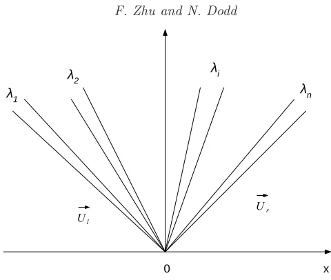
in which initial bed levels are not, in general, equal across the initial data: see figure 70

1. Aside from being important in the context of true dam-break events, they also have 71

relevance in the dynamics of waves on a beach. This is because a so-called backwash bore 72

(i.e., a hydraulic jump) is frequently created when water runs back down the beach after 73

a single wave uprush (Hibberd & Peregrine 1979). As the water drains the conditions at 74

the hydraulic jump may be such that flow is minimal and thus subsequent development 75

is predictable as a solution to a mobile-bed dam-break problem (Zhu & Dodd 2015). 76

Furthermore, we reconsider the usual shock conditions. For non-constant bed-levels 77

the bed-slope term in the flux-conservative form of the momentum equation is not in-78

tegrable, necessitating approximation using conditions on each side of the shock. Here 79

we reinterpret this term based on a new approximation of the internal shock structure. 80

Although the motivation for this comes from the limiting case of flow over a sloping 81

bed (and against which we subsequently verify the method), we instead approximate the 82

internal morphodynamic shock structure as a series of sub-shock problems. 83

In the next section we present our governing equations, as well as some of the theory 84

governing the determination of the wave structure across the evolving Riemann solution. 85

We then use this theory to solve this class of Riemann problem in§3. Finally we present 86

Dam

ˆ

hl

ˆ

ul= 0

ˆ

hr

ˆ

Br

ˆ

ur= 0

ˆ

Bl

ˆ

x= 0 xˆ

Figure 1.Schematic diagram for a dam-break problem.

2. Model development

2.1. Governing equations

89

A one dimensional (1D) idealised configuration for the initial set-up of a generalised dam-90

break problem is shown in figure 1. As mentioned, the nonlinear shallow water equations 91

(NSWEs) have often been used for describing one- or two-dimensional dam-break flows 92

(Ritter 1892; Stoker 1957; Toro 2001; Bernetti et al. 2008). For dam-break problems 93

over a mobile bed, and if only bed load is considered (see Soulsby 1997), the governing 94

equations are the NSWEs and a sediment conservation equation: 95

ˆ

htˆ+ ˆuhˆxˆ+ ˆhuˆxˆ= 0, (2.1)

ˆ

uˆt+ ˆuuˆxˆ+ghˆxˆ+gBˆxˆ= 0, (2.2)

ˆ

Bˆt+ξqˆxˆ= 0, (2.3)

where ˆxrepresents horizontal distance (m), ˆt is time (s), ˆhrepresents water depth (m), 96

ˆ

uis a depth-averaged horizontal velocity (ms−1_{), ˆB is the bed level (m), ˆq is sediment}

97

flux due to bed load (m2_s−1_),ξ= 1

1−p with pbeing bed porosity, andg is acceleration

98

due to gravity (ms−2_).

99

In order to reveal the shock dynamics by solving a strictly hyperbolic system, we do 100

not include the downslope diffusion effect in our model, although morphodynamic shocks 101

are considered where vertical bed steps occur. 102

In general, ˆqis strongly dependent on ˆuand a weak function of ˆh. Here, a simple but 103

commonly used formula ˆq=Auˆ3 _{(see Grass 1981) is employed for the bed load (see e.g.}

104

Kelly & Dodd 2010; Zhu et al. 2012), withAbeing the bed mobility parameter (s2_m−1_).

105

Note that this formulation is an over-simplification of the complex process of bed-load 106

transport (see e.g. Pritchard & Hogg 2005) but that the purpose here is to construct the 107

mathematical solution so that the basic dynamics can be understood, and to provide a 108

mathematical test case for numerical models. 109

Therefore, (2.3) becomes 110

ˆ

Bˆt+ 3ξAˆu2uˆxˆ= 0. (2.4)

2.2. Non-dimensionalisation

111

The nondimensional variables are 112

x= xˆ ˆ

h0

, t= ˆt ˆ

h1₀/2g−1/2, h=

ˆ

h

ˆ

h0

, u= uˆ ˆ

u0

and B = Bˆ ˆ

h0

where ˆh0is a length scale, and ˆu0= (gˆh0)1/2.

113

Substituting (2.5) into the governing equations (2.1), (2.2) and (2.4) gives 114

ht+uhx+hux= 0, (2.6)

ut+uux+hx+Bx= 0, (2.7)

Bt+ 3σu2ux= 0, (2.8)

whereσ=ξAg. 115

The vector form of these three non-dimensional governing equations is 116

~

Ut+A(U~)U~x= 0 (2.9)

with 117

~ U =





h u B



,A(U~) = 



u h 0

1 u 1

0 3σu2 ₀ 

.

The eigenvalues ofAare the roots of the polynomial equation 118

λ3−2uλ2+ (u2−3σu2−h)λ+ 3σu3= 0. (2.10)

Equation (2.10) has three roots, denotedλ1,λ2 andλ3 such thatλ16λ36λ2. For the

119

solution ofλ1,λ2andλ3 we refer to Kelly & Dodd (2009, 2010).

120

2.3. Generalised simple wave theory

121

When there are two equations or fewer in a Riemann problem, we can derive a Riemann 122

invariant along each characteristic (Stoker 1957). Jeffrey (1976) shows, however, that a 123

direct extension of the concept of a Riemann invariant is not possible when there are 124

more than two equations and dependent variables in a Riemann problem. Therefore, the 125

generalised simple wave theory and the generalised Riemann invariants are introduced 126

to solve such Riemann problems. 127

If we consider, for the moment, a general quasilinear hyperbolic system 128

~

Ut+A(U~)U~x= 0, (2.11)

whereU~ is a vector ofndependent variables, given by 129

~

U = [u1, u2, . . . , un]T, (2.12)

then the assumption that a simple wave region exists in a Riemann problem (or indeed 130

generally) is such thatU~ =U~(u1) holds across a wave, whereu1 is chosen without loss

131

of generality. This means that there is a functional dependence betweenui andu1of the

132

formui=fi(u1), and the wave is called a generalised simple wave (Jeffrey 1976). For a

133

simple wave, Eq. (2.11) can be written as, 134

_∂u

1

∂t I+ ∂u1

∂x A

_d~U

du1

= 0. (2.13)

This system can have a non-trivial solution ford~U /du1 only if

135

|A₋λiI|= 0, (2.14)

where 136

λi=−

_∂u

1

∂t

_∂u

1

∂x

, i= 1,2, . . . , n⇒ du_dt1 = 0 along dx

This implies thatu1, and thereforeui, are constant along characteristics dx_dt =λi, which

137

are themselves straight lines. A simple wave can also be defined as the wave, across which 138

one family of characteristics are all straight lines. There arenfamilies of characteristics, 139

and the simple wave associated with theith _{characteristic family is called theλ}

i simple

140

wave. 141

From Eq. (2.13), whenλ=λi the vector _dud ~U

1 must be proportional to the right eigen-142

vectorR~(i)_{of A, which gives (Jeffrey 1976),}

143

duj =

r(_ji)

r(1i)

du1, j= 2, . . . , n, (2.16)

wherer(_ji)is thejth component ofR~(i)_.

144

Integrating (2.16) yields thejth generalised Riemann invariantKjassociated with the

145

λi simple wave:

146

uj−

Z r(i)

j

r₁(i)du1=Kj, j= 2, . . . , n. (2.17)

Further details of the simple wave theory can be found in Jeffrey (1976). 147

Returning to the present system we have: 148

~ R(i)=





1

λi−u h

(λi−u)2

h −1



, (2.18)

and

du=λi−u

h dh (2.19)

dB=

_(λ

i−u)2

h −1

dh (2.20)

For a fixed t, where h varies continuously, Eqs. (2.19) and (2.20) may be integrated 149

across theλi simple wave, in the (h,u,B) phase space, to yield the structure. However,

150

variables do not always vary continuously across the Riemann structure. Therefore, we 151

must understand the structure before we can solve it. 152

2.4. Wave structure for a Riemann problem

153

In general the Riemann problem associated with Eq. (2.11), is composed of n waves 154

associated with thencharacteristic families, which are separated byn−1 newly formed 155

constant regions provided that the values in the initial piecewise constant states are 156

sufficiently close (Toro 2009; Lax 1973; Fraccarollo & Capart 2002): see figure 2. Note 157

that a wave could be a rarefaction fan, a shock, or a contact wave. 158

As we integrate Eqs. (2.19) and (2.20) across a λi simple wave, λi varies such that

159

dλi =P_∂uj∂λiduj, and in view of Eq. (2.16):

160

dλi

du1

=∇~_U~λi·R~(i) (2.21)

where we have assumed, without loss of generality, that r1(i) = 1. Eq. (2.21) therefore

161

represents the rate of change of characteristic velocity across theλi wave. If

162

~

Figure 2.Wave structure for a Riemann problem withncharacteristic families.

then the characteristic velocity increases or decreases continuously across theλi wave,

163

thus implying the existence of either an expansion (rarefaction) wave, or a compressive 164

wave (which becomes a shock ultimately). Then theλi wave field is said to be genuinely

165

nonlinear (or convex) (Sharma 2010). Note that if 166

~

∇U~λi·R~(i)= 0, for allU ,~ (2.23)

the wave field is said to be genuinely linear. 167

If we return again to the present system we find that 168

~

∇_U~λi·R~(i)=

λi+2λ2i −(2u−6σu)λi−9σu2 (u−λi)

h

G (2.24)

whereG= 3λ2_{−4uλ+ (u}2_−3σu2_{−h), and it is therefore not clear that (2.24) will be}

169

strictly>or<0. In this case the problem is said to be non-convex (Sharma 2010). Note 170

that this is in contrast to the classical (fixed bed) shallow water system, wherein 171

~

∇_U~λ−,+·R~(−,+)=∓

3 2

r

1

h. (2.25)

This implies that the solution to the dam-break problem resulting from the system (2.6)– 172

(2.8) may possess semi-characteristic shocks (Sharma 2010). 173

2.5. Semi-characteristic shock

174

In general, ∇~U~λi ·R~(i) = f(u1) across a simple wave. If, as seems possible for Eq.

175

(2.24),f(u1) passes through 0, this implies that at a rarefaction fan, across which

char-176

acteristics must diverge, a point is reached at which this can no longer happen because 177

dλi

du₁ = f(u1) = 0. The only way then of accommodating this behaviour without the

178

solution becoming multivalued is for a shock to be contiguous with the fan: the semi-179

characteristic shock, with the characteristic at one edge of the fan coinciding with this 180

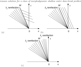
semi-characteristic shock. The possible three wave structures are shown in figure 3. Note 181

that only (a) represents a physical structure in general. This is because for figure 3(b) and 182

(c) the structures will, in general, be overdetermined. For further details and exceptions 183

(a) (b)

(c)

Figure 3.Schematic diagrams depicting possible structures for the combination of a rarefaction wave and a semi-characteristic shock within a simple wave.

2.6. Shock conditions

185

We require shock conditions to be satisfied across shocks and semi-characteristic shocks. 186

For derivations of the shock conditions we refer to Kelly & Dodd (2010); Zhu et al. (2012); 187

the shock conditions are 188

hRuR−hLuL−(hR−hL)W = 0, (2.26)

W(hRuR−hLuL)−

hRu2R+

h2

R

2 −hLu

2

L−

h2

L

2

−

Z xR

xL

hBxdx= 0, (2.27)

(BR−BL)W−σ(u3R−u3L) = 0, (2.28)

whereLandR represent variables on the left and right side of a shock, andW is shock 189

velocity. 190

The term RxR

xL hBxdx =

RBR

BL hdB is not uniquely determined, because h(x, t) is not

191

well defined along the face of bed step (Kelly 2009). Needham & Hey (1991) performed 192

the integration by approximation: 193

Z BR

BL

hdB≈1

2(BR−BL)(hR+hL). (2.29)

This expression is adopted by Kelly & Dodd (2010); Zhu et al. (2012); Zhu & Dodd 194

(2013, 2015). 195

step by the water: 197

Z BR

BL

hdB=



   

    1

2h

2

L ifBL+hL6BR

1

2(BR−BL)(2hL+BL−BR) ifBR >BL andBL+hL> BR

1

2(BR−BL)(2hR+BR−BL) ifBR < BL andBR+hR> BL 1

2h2R ifBR+hR6BL

(2.30)

There are four cases depending on from which side the water is exerting force on the 198

bed step, and whether the free surface on the side of lower bed level is above the top of 199

the bed step. Note that when free surface elevations on both sides are equal, Eqs. (2.29) 200

and (2.30) are identical. 201

Different interpretations are possible. This can be seen by assuming that in the vicinity 202

of a sudden change in bed level (a bed step)B =BL+ (BR−BL)H(x−x0), whereH(x)

203

is the Heaviside function, so that 204

Bx= (BR−BL)δ(x−x0) (2.31)

whereδ(x−x0) is the Dirac delta function, andx=x0 is the location of the bed step.

205

Using (2.31) 206

Z xR

xL

hBxdx= (BR−BL)h(x0). (2.32)

Therefore, the remaining ambiguity is in how to defineh(x0). From this perspective the

207

expression of Needham & Hey (1991) (hereinafter NH91) is a simple average depth across 208

the discontinuity; similarly, the middle two of the expressions of Bernetti et al. (2008) 209

also correspond to composite depths, although the first and last cannot obviously be 210

interpreted in this way. More generally, there is an implied variation of depth across the 211

shock, which, it turns out, is important for the shocks we consider here. 212

2.7. Investigation ofRxR

xL hBxdx

213

If we know the internal structure of a shock, i.e., h = h(B) across the shock, we can 214

calculate the ambiguous integral numerically or analytically straightforwardly: 215

Z BR

BL

hdB≈ n−1 X

i=0

¯

hi∆Bi= n−1 X

i=0

1

2(hi+hi+1) (Bi+1−Bi), (2.33)

wherehi =h(Bi),B0≡BL,Bn ≡BR, and here we take ∆Bi = BR−_nBL. Whenn= 1,

216

it is Needham & Hey (1991) approximation, i.e., (2.29). We refer to this approach as the 217

n-step approach; it is based on an implied internal structure of a shock. To see how this 218

internal structure might be arrived at from a physical standpoint we now consider flow 219

over a fixed bed slope. 220

2.7.1. Interpretation of a stationary shock across a fixed bed discontinuity

221

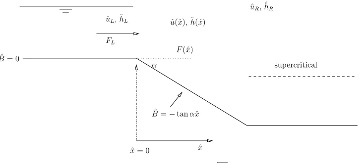
We consider a steady state flow across a fixed, linear slope (see figure 4), and therefore 222

only the hydrodynamic behaviour. From shallow water theory, the flow over the slope 223

is either entirely sub- or supercritical (see Appendix D). We return here to dimensional 224

variables, and then use an alternative non-dimensionalisation. 225

From continuity we have 226

ˆ

subcritical

supercritical

α

ˆ

B= 0

FL

F(ˆx)

ˆ

uR, ˆhR

ˆ

u(ˆx), ˆh(ˆx)

ˆ

B=−tanαxˆ

ˆ

x= 0 xˆ

ˆ

uL, ˆhL

Figure 4.Bed level geometry for this case.F = ˆu/

q

gˆhis the Froude number. In these scenarios the whole flow is either sub- or supercritical.

For a steady state, the flux-conservative form of (2.2) is 227

ˆ

huˆ2+1 2gˆh

2

ˆ

x

=−gˆhBˆˆx. (2.35)

Now we introduce a different set of nondimensional variables ˜h, ˜u, ˜xand ˜Bon the sloping 228

section with ˆh= ˆhL˜h, ˆu= ˆuLu˜, ˆx= ˆhLx/˜ tanα, and ˆB= ˆhLB˜. This gives:

229

˜

u= 1_˜

h, (2.36)

230

˜

B=−x,˜ (2.37)

and 231

FL2

1 ˜

h+

1 2˜h

2

˜

x

=−˜hB˜x˜= ˜h. (2.38)

Note that the slope tanαis now absent, and the only free parameter is the inflow Froude 232

number,FL.

233

Straightforwardly, we then obtain 234

˜

h= 1 + ˜x+1 2F

2

L

(˜h2−1) ˜

h2 = 1−B˜+

1 2F

2

L

(˜h2−1) ˜

h2 (2.39)

for the variation of ˜hacross the slope. If we consider an abrupt change in bed level to 235

be the limiting case asα→π/2 of this linear slope variation, and, moreover, that this 236

variation is independent of slope (tanα), we may then assume that this variation may 237

be used across a fixed bed step as the implied internal shock structure. 238

It should be noted that (2.39) can also be directly derived from an energy conservation 239

law for the shallow water equations, because the flow down the slope is continuous. There 240

is some debate about whether energy conservation or the momentum balance equation, 241

in whichRBR˜ ˜

BL

˜

hdB˜ has to be approximated, should be used for the shock across a fixed 242

has been widely used to study the stationary shock across a fixed bed discontinuity 244

(Karelskii & Petrosyan 2006; Valiani & Caleffi 2017). Valiani & Caleffi (2017) uses both 245

energy conservation and momentum balance to derive a depth at the bed step, i.e.,h(x0)

246

in (2.32). However, the energy loss across a morphodynamic shock isa priori unknown. 247

Therefore in this work, we utilise the momentum equation to solve the stationary shock 248

across a fixed bed step and also for morphodynamic shocks. Accordingly, we now focus 249

on the approximations forRBR˜ ˜

BL ˜hdB˜.

250

(2.38) gives the exact solution of 251

Z BR˜

˜

BL

˜

hdB˜=−

FL2

1 ˜

h+

1 2˜h

2

R

L

, (2.40)

for a stationary shock across a fixed bed discontinuity, in which ˜h is calculated using 252

(2.39). 253

The exact solution (2.40) together with (2.39) allows us to see how well (2.29), (2.30) 254

or (2.33) describe this usually ambiguous integral. The performances of these approxi-255

mations are presented in Appendix A, from which we can see that (2.33) yields greater 256

accuracy than (2.29) or (2.30). 257

2.7.2. Application ofn-step approach to morphodynamic shocks

258

In this section we consider whether the n-step approach is valid for morphodynamic 259

shocks. Hereafter we return to the non-dimensionalisation introduced in§2.2. 260

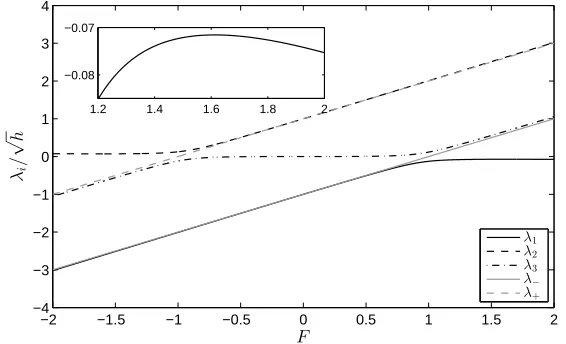
In the shallow water morphodynamical system that we consider here, there is in general 261

one characteristic speed much smaller than the other two. This can be seen in figure 5, in 262

which we plotλ′_=λ/√_{hversus Froude numberF=u/}√_{h. Note that the characteristic} 263

polynomial forλ′ _{depends only on F andσ:} 264

λ′3_{−2F λ}′2_{+ ((1−3σ)F}2

−1)λ′_{+ 3σF}3_{= 0. (2.41)}

The characteristic speed that is generally much smaller than the other two is associated 265

with bed wave movement. This property pertains everywhere except for transcritical 266

flows, as also indicated in figure 5. Here we define a morphodynamic shock as a shock 267

formed by the convergence of two characteristics of one family, at least one of which is a 268

bed characteristic, and for which the shock speed|W| ≪1. 269

Now, note thatσ=ξAg≪1 (see (2.8) and (2.28)). This is because ˆq=O(10−3_)m3_/s/m

270

or less, whereas ˆu0=O(1m/s) in our original non-dimensionalisation (2.5). This implies

271

that at the hydrodynamical timescale ˆt0 = q

ˆ

h0/g, (2.8) becomes Bt≈0, implying no

272

bed change at this timescale. However, at the morphodynamical timescale, ˆtm = ˆt0/σ,

273

⇒both sides of (2.28) are of comparable magnitude. This is consistent withW ≪1 for 274

a morphodynamic shock, so that in these circumstances (2.26)–(2.28) become 275

hRuR−hLuL≈0, (2.42)

−

hRu2R+

h2

R

2 −hLu

2

L−

h2

L

2

−

Z xR

xL

hBxdx≈0, (2.43)

(BR−BL)W−σ(u3R−u3L) = 0.

Note that (2.42) and (2.43) are the same shock conditions as those for flow over a fixed bed 276

step. This implies (2.39) can be derived from (2.42) and (2.43). This scaling is equivalent 277

to use of the quasi-steady approximation that is often used to study morphodynamics 278

(see e.g. Ribas et al. 2015). Therefore, we conclude that both (2.40) together with (2.39), 279

−2 −1.5 −1 −0.5 0 0.5 1 1.5 2 −4

−3 −2 −1 0 1 2 3 4

F

λi

/

√

h

λ₁ λ₂ λ₃ λ

− λ₊

1.2 1.4 1.6 1.8 2

−0.08 −0.07

Figure 5. Dimensionless characteristic velocities for our system with σ = 0.01 (after Zhu & Dodd (2015), figure 2). λ+,− are the equivalent hydrodynamic (fixed bed) characteristic velocities.

can in principle be used as approximations for morphodynamic shocks with simplified 281

shock conditions (2.42), (2.43) and (2.28). Note that the conversion between different 282

non-dimensionalisations in §2.7.1 and § 2.2 should be done before applying (2.40) and 283

(2.39) for morphodynamic shocks. 284

By analogy, we can instead retain the W terms in (2.26) and (2.27) to obtain the 285

internal shock structures (hi,uiandBi) and apply then-step approach (2.33) for (2.26)–

286

(2.28). In the remainder of this paper we use this approach, which we refer to as the 287

n-step approach, to construct the Riemann solution. The performances of these other 288

approximations for morphodynamic shocks are examined in Appendix C. 289

2.7.3. Implementation ofn-step approach for morphodynamic shocks

290

To use (2.33) across a morphodynamic shock with (2.26)–(2.28), the procedure is as 291

follows: 292

(a) Obtain initial estimates forU~R =U~_R(1) by solving (2.26)–(2.28), withR_xLxRhBxdx

293

approximated using (2.29). 294

(b) Bi values are then chosen according to BL and BR. Then h(Bi) and u(Bi) are

295

calculated according to (2.26) and (2.27) for the knownBi, by replacing (h, u, B)iL and

296

(h, u, B)iR by (h, u, B)i−1 and (h, u, B)i. Note that (h, u, B)0= (h, u, B)L.

297

(c) Calculate theRxR

xL hBxdxusing then-step approach (2.33).

298

(d) We then solve (2.26)–(2.28) using the calculatedRxR

xL hBxdxto get U~R=U~

(2)

R .

299

(e) Repeat (b)-(d) untilU~R converges.

300

3. Solution of dam-break problems over an initially piecewise flat

mobile bed

The dam-break problem system consists of 3 equations, and according to Lax’s theorem 303

(Lax 1973) there are at most 4 constant states separated by 3 elementary waves associated 304

with the 3 characteristic families. Note that for wet-dry dam-break problems over mobile 305

bed there are two waves separated by one newly formed constant region (Kelly & Dodd 306

3.1. Initial conditions

308

The dimensional initial conditions for a generalised dam-break problem are shown in 309

figure 1. With ˆh0= ˆhl, the non-dimensional initial conditions of the left side areh(x6

310

0) =hl = 1,u(x60) =ul= 0, B(x60) =Bl = 0. For wet-dry dam-break problems,

311

h(x> 0) =hr = 0, and u(x> 0) = ur = 0. For wet-wet dam-break problems, we set

312

h(x>0) =hr = 0.1, and u(x>0) =ur = 0. In this paper, we consider conditions of

313

both Br = 0 and Br 6= 0 to investigate the wave structures in these more generalised

314

dam-break problems. 315

3.2. Wet-dry dam-break problem

316

We first assume that the wet-dry dam-break solution over an erodible bed for various 317

Br consists only of elementary waves, i.e., rarefaction waves or shocks. We introduce

318

the semi-characteristic shock when the assumption no longer applies. The obtained wave 319

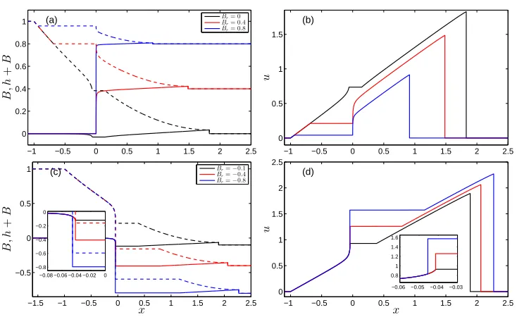
structures att= 1 are shown in figure 6. 320

3.2.1. Br>Bl

321

Figure 6(a) and (b) show, respectively, water surface elevation and bed level, and 322

velocity. The wave structure is that of aλ1 rarefaction wave, a constant region,U~∗, and 323

aλ3 rarefaction wave, which is consistent with that presented by Kelly & Dodd (2009),

324

who considered onlyBr=Bl= 0. AsBr→Bl+hl,B∗+h∗→Bl+hland the extents of

325

theλ1andλ3rarefaction waves decrease, and the solution (att= 1) resembles the initial

326

conditions more. Note that the volume of water set in motion at timetishl|λ1(hl)|t, and

327

is independent ofBrbecause the left edge of theλ1fan (λ1(hl)) is unaffected by changes

328

inBr. As the downstream elevationBrincreases, velocities across the Riemann solution

329

decrease, as, therefore, does the sediment movement. As Br increases, the flow in the

330

constant region changes from supercritical (e.g., whenBr = 0) to subcritical flow (e.g.,

331

when Br = 0.4 or 0.8), and the λ3 wave close to x = 0 changes from a hydrodynamic

332

into a bed wave. 333

In theλ3 rarefaction fan,

334

dB=

(λ3−u)2

h −1

dh=−3σu 2_(λ

3−u)

λ3h

dh (3.1)

where (2.10) has been used. Thus, the large bed change that occurs near the dam location 335

forBr= 0.4 or 0.8 is connected by the λ3 simple wave withλ3→0 in (3.1). The lip of

336

the initial bed discontinuity is eroded by the flow, and the initial discontinuity in bed 337

level is transformed into a steep continuous variation. The small bed step (Kelly & Dodd 338

2010) at the flow tip (x=xs(t)) remains a feature of the solutions with decreasing height

339

as flow velocity there decreases as Br increases. For Br =hl+Bl no flow ensues, and

340

there is no erosion. 341

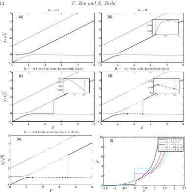
The wave development is closely related to Froude number (F), and Froude number 342

acts as a proxy for positionx. In figure 7(f), we show the relationship between F and 343

x. F increases across the Riemann solution as x increases. In figure 7 (a) and (b) the 344

three derived characteristic velocities λ′ _{= λ/}√_{h are plotted as a function of Froude} 345

number (F). Again, note that the λ′ _{curves are invariant for all dam-break solutions} 346

with σ= 0.01 unless there is a discontinuity in F when a shock develops. In contrast, 347

the black line superimposed on parts of these curves indicates the variation ofλ′

1across

348

the λ1 fan, and the variation of λ′3 across the λ3 fan, with the jump from one to the

349

other also depicted, forBr= 0 and 0.4. If we follow the (black)λ′i values along the λ′i

350

curves in figure 7 (a) and (b) from F = 0 we see that λ′

1 increases as F increases for

351

Br = 0.4 and 0. For Br = 0 the jump from λ′1 to λ′3 for Br >0, which corresponds

−1 −0.5 0 0.5 1 1.5 2 2.5 0

0.2 0.4 0.6 0.8 1

B

,h

+

B

(a) Br= 0

Br= 0.4 Br= 0.8

−1 −0.5 0 0.5 1 1.5 2 2.5

0 0.5 1 1.5

u

(b)

−1.5 −1 −0.5 0 0.5 1 1.5 2 2.5

−0.5 0 0.5 1

x

B

,h

+

B

(c) Br=−0.1 Br=−0.4 Br=−0.8

−0.08 −0.06 −0.04 −0.02 0 −0.8

−0.6 −0.4 −0.2 0

−1 −0.5 0 0.5 1 1.5 2 2.5

0 0.5 1 1.5 2 2.5

x

u

(d)

−0.06 −0.05 −0.04 −0.03 0.8

1 1.2 1.4 1.6

Figure 6.Structure of the wave solution for a wet-dry dam-break problem (hl = 1, ul = 0,

Bl= 0, hr = 0, ur = 0, andσ= 0.01) with varyingBr values (t= 1). All semi-characteristic shocks are solved by then-step approach for (2.26)–(2.28) with n= 2.

to the constant region, occurs for a largerF value than that forBr= 0.4. Both jumps

353

occur prior to the point at which dλ′1

dF = 0. Therefore,λ′ increases monotonically across

354

both fans. dλ′1

dF = 0, indicating a convergence inλ′1, occurs atF ≈1.6 for all dam-break

355

solutions withσ= 0.01. 356

3.2.2. Br6Bl

357

In figure 6(c) and (d) we can see the dam-break structure in this case, which is similar 358

to the preceding one in that two rarefaction fans (λ1 and λ3) form, separated by a

359

constant region. 360

Before commenting further on the structure of these solutions it is instructive first to 361

consider their representation in (λ′_{, F) space. In figure 7(c)-(e) we do this. Figure 7(c)} 362

and (d) illustrate the behaviour for Br =−0.4. For figure 7(c) we see the elementary

363

wave solution. Note, however, that the jump via the constant region, from λ′

1 to λ′3

364

curve, occurs when dλ′1

dF <0. This implies that at some point within the λ1 fan the λ′1

365

derived characteristics start decreasing asF increases. In contrast figure 7(d) shows the 366

behaviour with a semi-characteristic shock included. 367

Representing the solution in (λ′_{, F) space is appealing because these curves are} in-368

variant with the continuous Riemann solution (i.e. size of bed step). However, it is the 369

convergence of λ1 characteristics (not λ′1) in the (x, t)-plane that determines whether

370

or not a semi-characteristic shock must be fitted. So, to determine this point of change 371

in the Riemann solution it is appropriate to examine variation inλ1. The multivalued

372

solution ofλ1 starts atBr/−0.175, at the location at whichF ≈1.87 (andh≈0.301).

373

This point is illustrated in figure 8.λ1 increases asF increases, but atF ≈1.87 the the

374

characteristic velocity (λ1) starts to decrease at the leading edge of the λ1 rarefaction

375

fan. The constant region, corresponding to the jump from λ1 to λ3 curve, thus occurs

376

when dλ1

dF < 0. This indicates the convergence of λ1 characteristics within the λ1 fan.

377

The solution is multi-valued. The part of the λ1 curve for which F >1 behaves like a

0 1 2 3 4 5 −1

0 1 2 3 4 5

λ

/

√

h

Br= 0.4

(a)

0 1 2 3 4 5

−1 0 1 2 3 4 5

Br= 0

(b)

1 1.5 2 −0.09

−0.08

0 1 2 3 4 5

−1 0 1 2 3 4 5

F

λ

/

√

h

Br=−0.4 (with no semi-characteristic shock)

(c)

1.5 2 2.5 −0.085

−0.08 −0.075 −0.07

0 1 2 3 4 5

−1 0 1 2 3 4 5

F

Br=−0.4 (with semi-characteristic shock)

(d)

1.5 2 2.5 −0.1

−0.08 −0.06

0 1 2 3 4 5

−1 0 1 2 3 4 5

F

λ

/

√

h

Br=−0.8 (with semi-characteristic shock)

(e)

−1.5 −1 −0.5 0 0.5 1 1.5 2 2.5

0 2 4 6 8 10

x

F

(f) Br= 0.4 in (a)

Br= 0 in (b)

Br=−0.4 in (c)

Br=−0.4 in (d)

Br=−0.8 in (e)

Figure 7.Illustrations of four of the Riemann solutions depicted in figure 6 in (λ/√h, F) space as the solution is traversed fromxlto xs. Dashed lines represent the jumps fromλ1 wave and

λ3wave. Dash-dotted lines represent the jump at the semi-characteristic shocks. (f) Illustration

of howF varies across these solutions.

characteristic associated with a bed wave. Becauseλ1<0 this behaviour results in a bed

379

wave propagating against the flow. Similar behaviour can be observed in the propagation 380

of anti-dunes in supercritical open channel flow on a mobile bed, which propagate against 381

the flow (see Kennedy 1963). 382

To obtain a valid mathematical structure here, theλ1fan must terminate prior to the

383

point at which dλ1

dh = 0 at a semi-characteristic shock withλ1L=W; downstream, in the

384

constant region we must haveλ1R < W, for a valid shock structure, which is possible

385

becauseF increases across the shock and thereforeλ1 decreases.

386

Physically, the main difference between this case and that for Br > Bl is the larger

387

velocities induced by the lower downstream elevation, which drives the early supercritical 388

flow development and therefore the formation of the semi-characteristic shock. Now, the 389

constant region is shifted mostly to x > 0, with a large decrease in h_∗. The flow is 390

supercritical at the dam location, and the λ1 wave has become a bed wave close to

0 1 2 3 4 5 −1

−0.5 0 0.5 1 1.5 2

F

λ

Br=−0.175 (no semi-characteristic shock)

(a)

1.868 1.87 1.872 1.874 1.876 −0.0403

0 1 2 3 4 5

−1 −0.5 0 0.5 1 1.5 2

F

Br=−0.175 (with semi-characteristic shock)

(b)

1.87 1.875 1.88 −0.0403

0 0.2 0.4 0.6 0.8 1

−1 −0.5 0 0.5 1 1.5 2

h

λ

Br=−0.175 (no semi-characteristic shock)

(c)

0.3002 0.3004 0.3006 0.3008 0.301 −0.0403

0 0.2 0.4 0.6 0.8 1

−1 −0.5 0 0.5 1 1.5 2

h

Br=−0.175 (with semi-characteristic shock)

(d)

0.3 0.3005 0.301 0.3015 −0.0403

Figure 8.Illustrations of Riemann solutions for dam-break problem withhl= 1,ul= 0,Bl= 0,

hr= 0,ur= 0,Br= 0.175, andσ= 0.01 in (λ, F) and (λ, h) space to indicate why a semi-char-acteristic shock must be fitted. Dashed lines represent the jumps from λ1 wave and λ3 wave.

Dash-dotted lines represent the jump at the semi-characteristic shocks. All semi-characteristic shocks are solved by then-step approach for (2.26)–(2.28) with n= 2.

x= 0, where we can also see the large bed change. The large bed decrease occurs at the 392

shock, which helps to connect widely separated values ofBl andBr.

393

We assume an implied internal shock structure for all the semi-characteristic shocks, 394

andn= 2 is adopted here. For the semi-characteristic shocks for all negativeBr values,

395

we have λ1L = W > λ1R. The convergence of characteristics implies that the shocks

396

are physical. Note that if we use the approximation (2.29) we do not arrive at physical 397

solutions forBr=−0.8, and if we use the approximation (2.30) we do not get solutions

398

for any semi-characteristic shocks with the examined Br values. It is therefore critical

399

that we introduce this more accurate approach. In Appendix C we show the equivalent 400

solutions and examine dependence onn. 401

3.2.3. Varying upstream bed level

402

We also examine the effect of varying the upstream bed level only, while keeping the 403

upstream surface elevation and downstream bed level fixed (hl+Bl = 1 and Br = 0).

404

The Riemann solutions (B and B+h only) are shown in figure 9. The structures are 405

similar to those already observed, but now with particularly large variations between 406

solutions forx <0, becausehl varies and so therefore does the driving force.

407

The wave solutions of these dam-break problems are similar to those of fixed hl and

408

Bl values (hl = 1, Bl = 0) but varying Br values. Actually, these two kinds of

dam-409

break problems can be converted to each other through scaling and transformation. It 410

is the water depth on the left and bed difference that determines the wave structure. 411

Two dam-break problems with the same ratios of water depths and bed differences, i.e., 412

hl1/hl2= (Bl1−Br1)/(Bl2−Br2) are similar. Therefore the wave structures after dam

413

−1.5 −1 −0.5 0 0.5 1 1.5 2 2.5 0

0.2 0.4 0.6 0.8 1

x

B

,h

+

B

(a) Bl= 0.4

Bl= 0.2

Bl= 0

−1.5 −1 −0.5 0 0.5 1 1.5 2 2.5

−0.8 −0.6 −0.4 −0.2 0 0.2 0.4 0.6 0.8 1 1.2

x

(b) Bl= 0

Bl=−0.4

Bl=−0.8

Figure 9.Solutions for dam-break problems with fixed upstream surface elevation (hl+Bl= 1) and downstream bed level (Br = 0) but varyingBl values. All semi-characteristic shocks are solved by then-step approach for (2.26)–(2.28) withn= 2.

3.3. Wet-wet dam-break problem

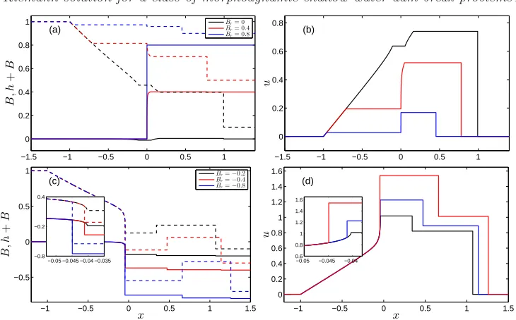
415

We now turn to the wet-wet dam-break solution over an initially piecewise flat erodible 416

bed for variousBrvalues, which consists of elementary waves. The solutions att= 1 are

417

shown in figure 10. 418

3.3.1. Br>Bl

419

Figure 10(a) and (b) show, respectively, water surface level and bed level, and velocity 420

for this case. The wave structure is of aλ1 rarefaction wave, a λ3 rarefaction wave and

421

a λ2 shock. There are two newly formed constant regions (U~l∗ and U~r∗) separating the 422

three waves. ForBr= 0, theλ2shock corresponds to theλ+shock in the equivalent fixed

423

bed wet-wet dam-break problem (e.g. Toro 2001), and theλ1 and λ3 rarefaction waves

424

correspond to the λ₋ rarefaction wave in the fixed bed case. When the bed mobility 425

σ→0, the λ1 andλ3rarefaction waves tend to combine into one wave.

426

AsBrincreases, theλ3 wave becomes more confined to the original bed step position,

427

and less water flows intox >0 region. Whenhr+Br→1 flow ceases.

428

3.3.2. Br6Bl

429

In figure 10(c) and (d), we can see the dam-break structure in this case. There is still 430

a λ1 rarefaction wave, and a λ2 shock, as for Br > Bl. However, for the investigated

431

negativeBrvalues, theλ3 wave changes from a rarefaction wave into a shock. There are

432

also two newly formed constant regions. ForBr <0 asBr decreases further (see figure

433

10(c)),hl∗ decreases very quickly, and whenhl∗< hr∗ theλ3fan observable for Br= 0

434

becomes a shock as the characteristics converge. 435

WhenBr/−0.207, we get multivalued solutions within theλ1 fan, (see figure 10(c)).

436

The Br value at which this occurs will depend on hr, which here is 0.1, recall. We

437

again assume the existence of aλ1semi-characteristic shock, and the corresponding wave

438

structure is shown in figure 10 (c) and (d). Once again, we assume an implied internal 439

shock structure, expressed through (2.33) in (2.26)–(2.28), in order to obtain a physical 440

shock (see Appendix C). 441

3.3.3. Varying downstream water depth

442

In figure 11 we look at the effect that varyinghrhas on the structure of these problems.

443

Ashrdecreases, we expect this wet-wet problem to start to resemble previously examined

444

wet-dry problems (see figure 6). Accordingly, theλ3 shock diminishes such that between

445

hr = 0.03 and 0.015 it becomes a rarefaction fan. As hr decreases further the λ3 fan

446

extends towards theλ2 shock such that in the limithr→0 the leading edge of thisλ3

−1.5 −1 −0.5 0 0.5 1 0

0.2 0.4 0.6 0.8 1

B

,h

+

B

(a) BBrr= 0= 0.4 Br= 0.8

−1.5 −1 −0.5 0 0.5 1

0 0.2 0.4 0.6 0.8

u

(b)

−1 −0.5 0 0.5 1 1.5

−0.5 0 0.5 1

x

B

,h

+

B

(c) BBrr==−−00..24 Br=−0.8

−0.05 −0.045 −0.04 −0.035 −0.8

−0.2 0.4

−1 −0.5 0 0.5 1 1.5

0 0.2 0.4 0.6 0.8 1 1.2 1.4 1.6

x

u

(d)

−0.05 −0.045 −0.04 0.6

0.8 1 1.2 1.4 1.6

Figure 10.Structure of the wave solution for a wet-wet dam-break problem (hl = 1,ul= 0,

Bl= 0,hr= 0.1,ur= 0, andσ= 0.01) with varyingBrvalues att= 1. All semi-characteristic shocks are solved by then-step approach for (2.26)–(2.28) with n= 2.

−1.5 −1 −0.5 0 0.5 1 1.5 2

−0.5 0 0.5 1

x

B

,h

+

B

(a) hhrr= 0= 0..103

hr= 0.015

0.6 0.65 0.7 0.75 0.8 −0.16

−0.14 −0.12 −0.1 −0.08

−1.5 −1 −0.5 0 0.5 1 1.5 2

−0.5 0 0.5 1

x

(b) hhrr= 0= 0..01001

hr= 0.0001

1.4 1.6 1.8 2

−0.4 −0.3 −0.2

Figure 11.Structure of the wave solution for a wet-wet Riemann problem with (hl= 1,

ul= 0,Bl= 0,ur= 0,Br=−0.4 andσ= 0.01) varyinghr values.

fan becomes the wet-dry boundary (with zero depth) and a semi-characteristic shock, and 448

theλ2shock disappears. Theλ1 wave is a combination of a fan and a semi-characteristic

449

shock, which is consistent with the equivalent wet-dry dam-break solution. 450

4. Conclusion

Generalised wet-dry and wet-wet dam-break problems over an erodible, initially piece-452

wise flat bed with water initially at rest and discontinuous bed levels are investigated and 453

solved based on the Riemann theory, and quasi-exact solutions are presented. The solu-454

tions are consistent with the theory proposed by Lax (1973) that for a Riemann problem 455

ofnequations there are at mostn+ 1 constant states separated bynelementary waves 456

associated with thencharacteristic families. However, for wet-dry dam-break problems, 457

one wave vanishes because of the presence of the dry bed. For the examined wet-dry 458

dam-break problems, there are 2 waves separated by 1 newly formed constant region, 459

For some dam-break problems with negative bed steps, in which the initial states (Bl

461

and Br) are not sufficiently close, there are multivalued solutions when applying Lax’s

462

theorem. The semi-characteristic shock is introduced to describe the flow and physical 463

wave structures are obtained. This is consistent with the solution for a Riemann problem 464

of one single equation of non-convex flux function (Sharma 2010). 465

The ambiguous integralRxR

xL hBxdxin shock conditions, which is usually approximated

466

by the Needham & Hey (1991) approach, is reconsidered. An implied internal shock struc-467

ture is proposed initially by considering the limiting case of flow down a linear slope over 468

fixed bed. Based on the internal shock structure, the integralRxR

xL hBxdx is discretized

469

into many steps and each step is approximated by Needham & Hey (1991) approach. 470

This is to reduce the effects of curvature betweenhandB, which is source of inaccuracy 471

in Needham & Hey (1991) approximation. This strategy is then extended to morphody-472

namic shocks which are here by assumption slow moving. However, because of the more 473

general implied internal shock structure approach we ultimately adopt it would appear 474

that this approach is more generally applicable. The resulting semi-characteristic shocks 475

are physical, in that the characteristics converge across them. 476

477

FZ and ND would like to acknowledge the financial support from both National Natural 478

Science Foundation of China (Grant No. 51509135) and University of Nottingham Ningbo 479

China (Small Research Grant). The authors would also like to thank the anonymous 480

reviewers for their constructive comments. 481

Appendix A. Analysis of

R

B_L

˜

hd

B

˜

approximation methods

482

In this section, we analyse the performances of three approximation methods for the 483

ambiguous termRB˜R

˜

BL ˜hdB˜ (in the orginal nondimensional system

RBR

BL hdBin shock

con-484

dition (2.27)) on a linear (fixed) slope in§2.7: (2.29), (2.30) and (2.33) with (2.39) against 485

the exact solution (2.40) with (2.39). 486

Here, we take ˜BL= 0 and ˜BR=−x˜, with ˜x >0 being a variable. The approximation

487

(2.29) gives 488

Z −x˜

0

˜

hdB˜ =−1₂x˜(1 + ˜h), (A 1)

and it is exact if the relationship between ˜hand ˜B is linear. The approximation (2.30) is 489

Z −x˜

0

˜

h dB˜=

(

−12x˜(2˜h−x˜) if ˜BR<B˜Land ˜BR+ ˜hR>B˜L

−1

2h˜

2 _{if ˜B}

R+ ˜hR<B˜L

(A 2)

We also use then-step approach (2.33) withn= 5 for the approximation 490

Z −x˜

0

˜

h dB˜ =−1

2

i=4 X

i=0

˜

hi+ ˜hi+1 B˜i+1−B˜i

(A 3)

with ˜Bi=−ix/˜ 5, in whichhi is calculated by (2.39).

491

The results of (A 1), (A 2), (A 3) and (2.40) are illustrated in figure 12. Comparison 492

shows that the approximation (A 1), i.e., (2.29), is generally quite accurate. Nearer to 493

critical conditions the free surface curvature introduces significant discrepancies. Also, as 494

˜

BR−B˜Lincreases, accuracy diminishes. Then-step approach (A 3), i.e., (2.33), greatly

495

increased the accuracy. The approximation (A 2), i.e., (2.30) (Bernetti et al. 2008), is 496

0 0.2 0.4 0.6 0.8 1 −2

−1.5 −1 −0.5 0

R˜BR ˜BL

˜hd ˜B

FL= 0.1

(a)

0 0.2 0.4 0.6 0.8 1 −2

−1.5 −1 −0.5 0

FL= 0.9

(b)

0 0.2 0.4 0.6 0.8 1 −0.8

−0.6 −0.4 −0.2 0

R˜BR ˜BL

˜hd ˜B

−( ˜BR−B˜L)

FL= 1.1

(c)

0 0.2 0.4 0.6 0.8 1 −1

−0.8 −0.6 −0.4 −0.2 0

−( ˜BR−B˜L)

FL= 2.1

(d)

Figure 12.RB˜R

˜

BL ˜

h dB˜plotted against size of bed step:RB˜R

˜

BL ˜

h dB˜=₋hF2

L

1 ˜

h+

1 2˜h

2iR

Lcalculated using (2.39) (solid black line); that approximated by (A 1), i.e., (2.29) (dashed line), by (A 2), i.e., (2.30) (dotted line), and by (A 3), i.e., (2.33) withn= 5 (grey solid line) for various Froude numbers.

the exact value when it is closer to critical flow. However, when the flow is supercritical, 498

the discrepancies become significant. 499

Appendix B. Comparison between wet-dry dam-break Riemann

solution of fixed and nearly fixed bed case

In this section, we test the Riemann solver by comparing the nearly fixed bed wet-dry 502

dam-break solution (σ= 1×10−5_{) against the fixed bed solution.}

503

The dam-break problem over a fixed bed with a bed step will lead to a stationary 504

shock at the bed step (Bernetti et al. 2008). For the positive Br values examined, the

505

wave structure over a fixed bed from the left to right is aλ−rarefaction wave, a constant 506

region, a stationary shock, and aλ− rarefaction wave. That for the negativeBr values

507

examined, is a λ₋ rarefaction wave, a stationary shock, a constant region, and a λ₋ 508

rarefaction wave (figure 13). This stationary shock corresponds to a semi-characteristic 509

shock if we interpret it in a morphodynamic context. It is aλ3 semi-characteristic shock

510

withλ3L =W =λ3R= 0 becauseσ= 0.

511

On a nearly fixed bed, the wave structure for the non-negativeBr values examined, is

512

aλ1rarefaction wave, a constant region and aλ3rarefaction wave. The stationary shock

513

in the fixed bed case disappears because of the bed mobility, and the left part of theλ3

−1 −0.5 0 0.5 1 1.5 2 2.5 3 0

0.2 0.4 0.6 0.8 1

x

B

,h

+

B

(a) Br= 0

Br= 0.2

Br= 0.4

Br= 0.6

Br= 0.8

−1 −0.5 0 0.5 1 1.5 2 2.5 3

−0.5 0 0.5 1

x

B

,h

+

B

(b) Br= 0

Br=−0.2 Br=−0.4 Br=−0.6 Br=−0.8

Figure 13.Comparison between wet-dry dam-break fixed bed (hl= 1,ul= 0,Bl= 0,hr= 0,

ur= 0, andBr= 0) solution (σ= 0; solid lines) and nearly fixed bed solution (σ= 1×10−5; dashed lines). All semi-characteristic shocks are solved with NH91 approximation.

rarefaction wave becomes a steep but smooth part, which is to some extent similar to 515

the stationary shock in the fixed bed case. The nearly fixed bed solutions are in good 516

agreement with the fixed bed solutions (figure 13(a)). 517

The Riemann solutions with NH91 condition for the examined negativeBrvalues over

518

a nearly fixed bed are similar to those presented in§3.2.2. The wave structures are aλ1

519

rarefaction, aλ1 semi-characteristic shock, and aλ3 rarefaction. Theλ1 rarefaction fan

520

corresponds to the stationary shock on the fixed bed. The results compare favourably 521

with the corresponding fixed bed results (figure 13(b)). 522

Appendix C. Investigation of

R

B_L

hdB

approximation methods in

523

dam-break problems

In this section, we investigate the approximation ofRBR

BL hdBby comparing the

solu-525

tions of wet-dry and wet-wet dam-break problems using different approximation methods 526

(see Appendix A and§2.7.2). In summary, the approximation methods include (a): (2.40) 527

together with (2.39) and (2.28), i.e.,hRanduRare directly calculated for a knownBRas

528

for the stationary shock across fixed bed discontinuity; (b):n-step approach with (2.39) 529

applied in (2.42), (2.43) and (2.28) (c):n-step approach with (2.26)-(2.27) forhi,ui and

530

Bi for (2.26)-(2.28), (d): NH91 approximation (i.e.,n-step approach in method (c) with

531

n= 1; and (e): Bernetti et al. (2008) condition for (2.26)-(2.28) It should be noted that 532

with Bernetti et al. (2008) condition, we cannot find a solution if a semi-characteristic 533

shock is assumed, i.e., there is no alternative to the multi-valued solution. 534

The performances of the approximation methods forRBR

BL hdBare compared by

exam-535

ining wet-dry dam-break solutions for bothBr=−0.4 and−0.8. In general, the

approx-536

imations give similar results for water levels and bed elevations when the whole solution 537

is shown. Differences can be seen at the semi-characteristic shock. When Br = −0.4,

538

method (a) and (b) give very similar results, and the results of method (c) and (d) 539

are close. When the bed step height increases, the difference grows. However, the semi-540

characteristic shocks predicted by method (a) and (b) for Br =−0.4 (and Br =−0.2,

541

not shown) and that by method (d) for Br = −0.8 (and Br = −0.6, not shown) are

542

non-physical becauseλ1L>W >λ1R cannot be satisfied. In contrast, method (c), used

543

throughout this paper, results in a physical semi-characteristic shock for all these Br

544

values. It is therefore necessary to retain theW terms in (2.26)-(2.28). 545

The effects of how many steps the integralRBR

BL hdBis discretized into are also

investi-546

gated. The comparison for both wet-dry and wet-wet dam-break problems using method 547

−1.5 −1 −0.5 0 0.5 1 1.5 2 2.5 −0.5

0 0.5 1

x

B

,h

+

B

Br=−0.4

(a) Method (a)Method (b)

Method (c) Method (d)

−0.055−0.05−0.045−0.04 −0.5

0 0.5

−1.5 −1 −0.5 0 0.5 1 1.5 2 2.5

−0.5 0 0.5 1

x

B

,h

+

B

Br=−0.8

(b) Method (a)Method (b)

Method (c) Method (d)

−0.055−0.05−0.045−0.04 −0.5

0 0.5

Figure 14. The comparison of wet-dry dam-break (hL = 1,uL= 0,BL= 0) solutions with different approximation methods forRBR

BL hdB. In then-step approach in method (b) and (c), n= 2.

that the results with the implied internal shock structure are initially very close to those 549

directly using the NH91 approximation. As the size of bed step increases, the difference 550

between solutions with NH91 approximation and the new approach also increases slightly. 551

In the wet-dry dam-break problems with Br = −0.2,−0.4, the semi-characteristic

552

shocks haveλ1L=W > λ1R when solved directly with NH91 approximation. However,

553

as previously mentioned that for Br = −0.6,−0.8, we have λ1L = W < λ1R, which

554

indicates a non-physical shock. It is further noted that in theBr=−0.4,−0.6,−0.8 cases,

555

the water on the left and right sides of the λ1 semi-characteristic shock are separated

556

by the high bed step (figure 16). Similarly, in the wet-wet dam-break problems with 557

Br=−0.6,−0.8, the semi-characteristic shocks are also non-physical. However, when we

558

use the implied internal shock structure, the shocks become physical. 559

In order to further investigate this, we take the wet-dry dam-break problem with 560

Br =−0.6 as an example to illustrate the characteristics across the semi-characteristic

561

shocks; see figure 17. We can see the characteristics diverging when using the NH91 ap-562

proximation, and characteristics converging when using implied internal shock structure. 563

This indicates that the NH91 approximation becomes less accurate when the bed step 564

becomes large in which the curvature ofh withB becomes enhanced. In this case, the 565

importance of considering the internal shock structure becomes obvious. 566

In figure 18 we see how the multivalued problem in a wet-dry dam-break problem is 567

rationalised by introducing a semi-characteristic shock. According to Whitham (1974), 568

the areas ∆A1= ∆A2. The results obtained here are consistent with this law, and when

569

n increases, |∆A1−∆A2| decreases. This also demonstrates that the n-step approach

570

applied for (2.26)-(2.28) gives more accuracy. Note that when the NH91 condition is used, 571

the jump at the semi-characteristic shock occurs outside the multi-valued region. As a 572

result, the shock becomes non-physical, becauseλ1_∗> λ1L=W.

573

Appendix D. Impossibility of a smooth flow from sub- to

supercriticality down a slope

For smooth transition from sub- to supercriticality down a slope we need a situation 576

like that depicted in figure 19. 577

This flow is described by (2.38). Note that the RHS of (2.38)>0 for all ˜x; therefore 578

−1.5 −1 −0.5 0 0.5 1 1.5 2 2.5 −0.5 0 0.5 1 x B ,h + B

Br=−0.2

(a) NH91n= 2

n= 4

n= 6

−0.0404 −0.0402 −0.04 −0.2

−0.1 0 0.1 0.2

−1.5 −1 −0.5 0 0.5 1 1.5 2 2.5

−0.5 0 0.5 1 x B ,h + B

Br=−0.4

(b) NH91n= 2

n= 4

n= 6

−0.06 −0.05 −0.04 −0.03 −0.5

0 0.5

−1.5 −1 −0.5 0 0.5 1 1.5 2 2.5

−0.5 0 0.5 1 x B ,h + B

Br=−0.6

(c) NH91n= 2

n= 4

n= 6

−0.06 −0.05 −0.04 −0.03 −0.5

0 0.5

−1.5 −1 −0.5 0 0.5 1 1.5 2 2.5

−0.5 0 0.5 1 x B ,h + B

Br=−0.8

(d) NH91n= 2

n= 4

n= 6

−0.06 −0.05 −0.04 −0.03 −0.5

0 0.5

−1.5 −1 −0.5 0 0.5 1 1.5 2

−0.5 0 0.5 1 x B ,h + B

Br=−0.4

(e) NH91n= 2

n= 4

n= 6

−0.06 −0.05 −0.04 −0.03 −0.5

0 0.5

−1.5 −1 −0.5 0 0.5 1 1.5 2 2.5

−0.5 0 0.5 1 x B ,h + B

Br=−0.6

(f) NH91n= 2

n= 4

n= 6

−0.06 −0.05 −0.04 −0.03 −0.5

0 0.5

−1.5 −1 −0.5 0 0.5 1 1.5 2

−0.5 0 0.5 1 x B ,h + B

Br=−0.8

(g) NH91n= 2

n= 4

n= 6

−0.06 −0.05 −0.04 −0.03 −0.5

0 0.5

Figure 15.The comparison of dam-break solutions with NH91 approximation and those with the implied internal shock structure (n-step approach, for various n values). (a)–(d): wet-dry dam-break solutions; (e)–(g): wet-wet dam-break solutions.

If we differentiate the LHS of (2.38) w.r.t.xwe get:

˜

h˜hx˜−FL2

˜

h˜x

˜

h2 =˜hx˜

˜

h−F 2

L

˜

h2

=˜h˜hx˜

−1.5 −1 −0.5 0 0.5 1 1.5 2 2.5 −0.5

0 0.5 1

x

B

,h

+

B

Figure 16. Structure of the wave solution (NH91 approximation) for a wet-dry dam-break problem withBr=−0.6 which shows that the water on the two sides of the semi-characteristic shock is separated by the high bed step (t= 1).

−20 −1.5 −1 −0.5 0 0.5 1 1.5 2

0.2 0.4 0.6 0.8 1

λ₁ fan Constant star region λ₃ fan

x

t

(a)

−0.037 −0.0365 −0.036 0.77

0.775 0.78 0.785 0.79

−20 −1.5 −1 −0.5 0 0.5 1 1.5 2

0.2 0.4 0.6 0.8 1

λ₁ fan Constant star region λ₃ fan

x (b)

−0.015 −0.01 −0.0050 0 0.1

0.2 0.3 0.4

Figure 17.The characteristics set up for the dam-break solutions withBr=−0.6 with NH91 approximation (a) and n-step approach applied for (2.26)-(2.28) (n= 2; b).

−1.5 −1 −0.5 0 0.5 1 1.5 2 2.5 0

0.2 0.4 0.6 0.8 1

x

h

Br=−0.6

No shock NH91

n= 2

n= 4

n= 6

−0.046 −0.044 −0.042 −0.04

0.25 0.3 0.35

∆A1

∆A2

Figure 18.Multivalued profile and semi-characteristic shock fitting with NH91 approximation andn-step approach (2.33) for (2.26)–(2.28) in a wet-dry dam-break solution withBr=−0.6.

However, for the flow in figure 19, ˜h˜x<0. Therefore, we must have

1−F 2

L

˜

FL

F

˜

uL,˜hL

˜

u,h˜

˜

h= ˜hc

Figure 19.Smooth flow on a constant slope from sub- to supercritical conditions.

Now,

F2=uˆ

2

ghˆ =

ˆ

u2

L

gˆhL

˜

u2

˜

h =F

2

L

1 ˜

h3 (D 3)

⇒

1−F 2

L

˜

h3

=

1−F2 (D 4)

Therefore, if flow is subcritical the flow cannot exist. Therefore, the flow in figure 19 580

cannot exist. The authors could not find an example in the literature of this analysis 581

being presented, hence its inclusion here. 582

REFERENCES

Bernetti, R., Titarev, V. A. & Toro, E. F.2008 Exact solution of the riemann problem for

583

the shallow water equations with discontinuous bottom geometry. J. Comput. Phys.227_, 584

3212–3243.

585

Cozzolino, L., Morte, R. D., Covelli, C., Giudice, G. D. & Pianese, D.2011 Numerical

586

solution of the discontinuous-bottom shallow-water equations with hydrostatic pressure

587

distribution at the step. Advances in Water Resources34_{, 1413–1426.} 588

Fraccarollo, L. & Capart, H.2002 Riemann wave descriptions of erosional dam break flows.

589

J. Fluid Mech.461_{, 183–228.} 590

Grass, A.J.1981 Sediment transport by waves and currents. Technical Report FL29. University

591

College London, London Centre for Marine Technology.

592

Hibberd, S. & Peregrine, D. H.1979 Surf and run-up on a beach: A uniform bore. J. Fluid

593

Mech.95_{, 323–345.} 594

Jeffrey, A.1976 Quasilinear hyperbolic systems and waves. Pitman.

595

Karelskii, K. V. & Petrosyan, A. S.2006 Problem of steady-state flow over a step in the

596

shallow-water approximation. Fluid Dynamics41_{(1), 12–20.} 597

Kelly, D. M.2009 Bore-driven swash on a mobile beach. PhD thesis, School of Civil

Engineer-598

ing, University of Nottingham, Nottingham, UK.

599

Kelly, D. M. & Dodd, N.2009 Floating grid characteristics method for unsteady flow over a

600

mobile bed. Computers and Fluids38_{, 899–909.} 601

Kelly, D. M. & Dodd, N.2010 Beach face evolution in the swash zone. J. Fluid Mech.661_, 602

316–340.

603

Kennedy, J. F.1963 The mechanics of dunes and antidunes in erodible-bed channels. J. Fluid

604

Mech.16_{(4), 521–544.} 605

Lax, P. D.1973 Hyperbolic systems of conservation laws and the mathematical theory of shock

606

waves. S.I.A.M.

Needham, D. J. & Hey, R. D.1991 On nonlinear simple waves in alluvial river flows: a theory

608

for sediment bores. Phil. Trans. Roy. Soc. Lond. A334_{, 25–53.} 609

Pritchard, D. & Hogg, A. J.2005 On the transport of suspended sediment by a swash event

610

on a plane beach. Coastal Eng.52_{, 1–23.} 611

Ribas, F., Falqu´es, A., de Swart, H. E., Dodd, N., Garnier, R. & Calvete, D.2015

Un-612

derstanding coastal morphodynamic patterns from depth-averaged sediment concentration.

613

Rev. Geophys.53_{, 362–410.} 614

Ritter, A.1892 Die fortpflanzung der wasserwellen. Vereine Deutcher Ingenieure Zeitschrift

615

36_{, 947–954.} 616

Sharma, V. D.2010 Quasilinear Hyperbolic Systems, Compressible Flows, and Waves. CRC

617

Press.

618

Soulsby, R. L.1997 Dynamics of marine sands. a manual for practical applications. SR 466.

619

Hydraulics Research Wallingford, Wallingford, England.

620

Stoker, J.J.1957 Water Waves. New York, N.Y.: Interscience.

621

Toro, E. F. 2001 Shock-capturing methods for free-surface shallow flows. New York, NY.:

622

Wiley.

623

Toro, E. F.2009 Riemann solvers and numerical methods for fluid dynamics, 3rd edn. Berlin:

624

Springer.

625

Valiani, A. & Caleffi, V.2017 Momentum balance in the shallow water equations on bottom

626

discontinuities. Advances in Water Resources100_{, 1–13.} 627

Whitham, G. B.1974 Linear and Nonlinear Waves. New York: Wiley-Interscience.

628

Zhu, F. & Dodd, N.2013 Net beach change in the swash: A numerical investigation. Advances

629

in Water Resources53_{, 12–22.} 630

Zhu, F. & Dodd, N. 2015 The morphodynamics of a swash event on an erodible beach. J.

631

Fluid Mech.762_{, 110–140.} 632

Zhu, F., Dodd, N. & Briganti, R.2012 Impact of a uniform bore on an erodible beach.

633