Colin Robertson1, Jed A. Long2, Farouk S. Nathoo3, Trisalyn A. Nelson2, Cameron C.F. Plouffe1 1
Department of Geography & Environmental Studies, Wilfrid Laurier University, 75 University Ave West, Waterloo, ON, N2L 3C5, Canada, 2Spatial Pattern Analysis & Research (SPAR) Laboratory, Department of Geography, University of Victoria, PO Box 3060, Victoria, BC V8W 3R4, Canada, 3Department of Mathematics & Statistics, University of Victoria, PO Box 3060, Victoria, BC V8W 3R4, Canada
Correspondence: Colin Robertson, Department of Geography & Environmental Studies, Wilfrid Laurier University, 75 University Ave West, Waterloo, ON, N2L 3C5, Canada
e-mail: [email protected]
Pre-print of published version.
Reference:
Robertson, C, JA Long, FS Nathoo, TA Nelson, CCF Plouffe. 2014. Assessing quality of spatial models using the structural similarity index and posterior predictive checks. Geographical Analysis. 46(1). 53-74.
DOI:
http://dx.doi.org/10.1111/gean.12028
Disclaimer:
1
Introduction
Models of spatially varying phenomena commonly incorporate spatially distributed model parameters to account for spatial variation in the relationship between a process and modeled or missing covariates (Finley 2011). For example, space-time models of dynamic processes such as infectious disease or invasive species spread, utilize spatially distributed model parameters to account for spatial heterogeneity in epidemic waves (e.g., Smith et al. 2002, Wheeler and Waller 2008). Statistical models with spatially-varying coefficients can accommodate non-stationary relationships in a regression context, which is particularly useful for large study areas. A key advantage of spatially explicit modelling for geographical analysis is that parameter estimates can be mapped and integrated with other spatial data sets. The most common approaches for modelling spatially heterogeneous processes include Bayesian hierarchical modelling with dynamic spatial models (Gelfand et al. 2003), geographically weighted regression (GWR) (Brundson, Fotheringham, and Charlton 1996) and spatial filtering methods (Griffith 2008).
2 determine the best model among a suite of candidate models, or to combine relative strengths of different models through model averaging (Burnham and Anderson 2002). The model selection stage provides little information about the overall quality of proposed models, requiring
alternative objective approaches for examining goodness-of-fit. For a recent example, Finely et al. (2012) use a squared error loss function that incorporates both discrepancy in the estimated values (i.e., mean) and uncertainty (i.e., variance) in predictions as model selection criteria within a posterior predictive model-checking framework.
The second stage of model assessment examines how well a selected candidate model agrees with data in order to quantify goodness-of-fit. A more expansive treatment of model residuals is typically conducted to quantify their magnitude and structure in a separate stage through goodness-of-fit tests. Typical approaches for measuring goodness-of-fit include a comparison of observed and estimated values, such as the chi-squared (χ2) test (e.g., Dice 1945), the root mean squared error, the mean absolute error (i.e., bias), or kappa statistics (e.g., Carletta 1996). These tests are undertaken in geographical analysis any time a researcher has observed and predicted values (e.g., spatial interpolation, hierarchical modelling, image classification). Because these methods are employed so widely in many areas of geography, we use the term ‘error’ here interchangeably with ‘residual’ rather than the more precise definition related to the
difference between an estimate and its true parameter value.
With analysis of spatial data, aspatial goodness-of-fit measures can be misleading,
3 details or confidence about model fit. Cliff and Ord (1981) employ global join-counts and
Moran’s statistics to measure spatial autocorrelation of observed and expected maps derived from simulations of Hagerstrand’s spatial diffusion model (Hägerstrand 1953). More recently,
Wulder et al. (2007) use a local measure of spatial autocorrelation to assess the spatial variation in error/variance in several scenarios of a forest productivity model; this practice is becoming increasingly common (e.g., Räty and Kangas 2010 ). Here we are concerned specifically with this second problem, and the continued development of spatially sensitive metrics for assessing model goodness-of-fit.
A number of problems exist with measures of model fit commonly applied to traditional spatial models; for example, the true values for spatial parameters are generally unknown. Typically, assumptions and estimates of true values are based on results of field experiments taken over limited spatial scales (e.g., Turchin and Thoeny 1993). Scaling up field experiments to large-area spatial models is extremely challenging because ground truth data for models using coarsely grained units, such as pixels of 1 km by 1 km or larger, are very difficult to obtain.
4 Spatially local assessment methods, or those that characterize the spatial pattern of parameter estimates, are beneficial because they reveal systematic errors and spatial variability in errors that can be used to further refine models.
Furthermore, because some variability in predictions is expected from all models (i.e., all models are wrong), determining when the difference between two maps is more than expected given a data generating spatial process can be problematic. For instance, often two maps generated as realizations of a spatial model are expected to have variability in output values at the same spatial location (Csillag and Boots 2005). This issue has been discussed mostly in the remote sensing literature, where traditionally researchers have set subjective thresholds above which change is considered substantive (Gong and Xu 2003).
In the last decade, map comparison research has begun to overcome several of the preceding issues. Map comparison techniques are useful for evaluating similarities and differences between two map patterns. Map comparison approaches have been developed primarily for measuring agreement between categorical maps (Boots and Csillag 2006; Hagen-Zanker 2006b; Visser and DeNijis 2006); for example, land-use and land-cover change
5 assessment of change in continuous-value maps, although Hagen-Zanker(2006a) reviews a suite of potential methods.
A final issue with assessing spatially explicit models is that the true values for the spatial process of interest often are unknown, and so must be estimated in some fashion. Frequently, hierarchical spatial models are fit within the Bayesian paradigm with implementation based on Markov chain Monte Carlo (MCMC) techniques. Within the Bayesian context,
posterior-predictive checking is a general approach to goodness-of-fit, whereby a fitted model, through its posterior distribution, is used to generate replicate data with the assumed model, where values are compared with observed data through a measure of discrepancy (Gelman, Meng, and Stern 1996). The combined methods described here represent a framework for checking spatial models, and provide a diagnostic tool to improve model-based spatial analysis.
In this paper, we employ a spatially explicit approach to evaluation of spatial models in a Bayesian model-checking framework. The primary contribution of this paper is a new model assessment methodology, based on two approaches: posterior predictive checks, and map comparison based on the structural similarity (SSIM) index, which are combined to quantify the spatial nature of a model fit. In short, fitted models are used to simulate new realizations of a process using its posterior predictive distribution, and these are compared to the observed data using spatially sensitive metrics. This approach is in line with the notion of a process-based approach to map comparison presented in Csillag and Boots (2005). The posterior predictive realizations from a fitted model can be interpreted as replicate data that could have been
6 approach with the SSIM index for checking the fit of spatial models. Because geographers
typically work with data that describe one instance of spatially stochastic processes, simulation-based inference is a powerful method for understanding geographic patterns.
Methods
Two component methods for the proposed model assessment approach are posterior predictive checks and map comparison. We briefly review each of these approaches before demonstrating their role in spatial model assessment.
Posterior Predictive Model Checking
Posterior predictive model checking differs from the classical hypothesis testing framework in that emphasis is placed on measuring the discrepancy between observed data and replicate data simulated with a fitted model, rather than testing whether the model is true or false. In Bayesian statistics, all parameters are treated as stochastic and assigned a prior distribution p(θ), and inference proceeds through the posterior distribution p(θ |Y), which conditions on observed data Y. For a given model, specified by a likelihood p(Y|θ) and a prior p(θ), the posterior predictive distribution
p Y d
Y p Y Y
p( rep | ) ( rep | ) ( | ) (1)
allows us to draw new replicate data from the fitted model. The replicate data Yrep are assumed
to have the same distribution as the observed data Y (which is specified as part of a model), and also assumed conditionally independent of Y, given θ. As described in Gelman, Meng, and Stern (1996), simulated realizations of Yrep can be compared to observed data through a general
discrepancy measure T(Yrep,Y). This discrepancy measure is a specifically chosen statistic that
7 measure for exploratory map comparison for continuous-valued spatial model assessment. In the analysis reported here, we simulate 100 Yrep datasets from fitted models, and then compare the
observed Y and Yrep datasets (i.e., Yrep vs, Y). Alternatively, in some cases the appropriate
comparison is between parameter estimates obtained from posterior distributions and their true
values (i.e.,
^
vs. ), to evaluate the fit of a specific model component. In all analyses, replicates
were generated by randomly drawing parameter values i from the posterior distribution , and using these to simulate new values (i.e., Yrep).
Map Comparison
We selected the SSIM index (Wang et al. 2004), developed for evaluating image degradation, as an exploratory map comparison statistic for use in continuous-valued spatial model assessment. The SSIM index was originally proposed for evaluating the quality of image compression algorithms, but was later identified as a potential method for comparing continuous valued maps by Hagen-Zanker (2006a). The SSIM index is constructed to objectively make comparisons between images similar to the human visual system. A comparison of the mean square error (MSE) and SSIM index in Wang et al. (2004) shows that for a fixed MSE, vastly different image degradations are possible from a human perception standpoint. We employ the SSIM index to extend this notion to map comparison for model checking. A local region approach is ideal for simultaneously assessing similarity in spatial structure along with pixel-by-pixel correspondence in maps (Hagen-Zanker and Martens 2008).
8 Three summary statistics used in calculating the SSIM index are computed for each cell on the basis of a defined local region (e.g., a 5x5 moving window).
n i i i
a w a
1
(2)
2
1 1 2
n i a i ia w a
(3)
n i b i a i iab w a b
1
(4)
In the preceding three equations, a and b are two regular lattice maps, the index i iterates through n cells in a defined local region, and wi are spatial weights that can be used to adjust the
smoothness/ abruptness of the local region effect. For example, in Wang et al. (2004), an 11x11 circular local region is used with Gaussian weights. For equal weights, all wi can be set to 1/n.
The local measures are combined into the three SSIM index components–luminance (L), contrast (C), and structure (S)–as follows:
1 2 2 1 2 c c ) b , a ( L b a b a (5) 2 2 2 2 2 c c ) b , a ( C b a b a (6) 3 3 c c ) b , a ( S b a ab (7)
where the constants c1, c2, and c3 are included for stability in situations where either the mean or
variability is close to zero (e.g., large homogeneous patches). These constants can be related to the range of pixel values (R) via two additional constants, k1 = 0.01 and k2 = 0.03, established
heuristically by Wang et al. (2004): c1 = (k1R)2, c2 = (k2R)2, and c3= ½ c2. Note that these three
9 necessarily affect the others. The components L and C fall in the interval [0,1] with 1 indicating perfect agreement, and S falls in the interval [-1,1] (the correlation coefficient between cells in each window). A value for the SSIM index of -1 indicates perfect negative correlation among values in the locally compared regions. The three SSIM index components are multiplicatively combined to give a measure of similarity for each local region that is equal to 1 when the two maps are identical:
)] b , a ( S [ )] b , a ( C [ )] b , a ( L [ ) b , a (
SSIM (8)
The exponents α, β, and γ can be used to weigh individual components, with default values taken as α = β = γ = 1. Interpreting maps of L, C, S and the SSIM index values allows spatially local
analysis of patterns of model fit. Alternatively, a global score of similarity (termed mSSIM) can be computed by taking the mean of all local SSIM index values. Global summaries can be calculated for each individual component. Given the structure of these formulas, the mSSIM value obtained by taking the mean of the local SSIM index values does not necessarily equal the product of the component global means.
Expected and observed maps with low similarity in L indicate a poorly estimated local mean, whereas disagreement in C may indicate that local transitions are different across
10 predictive distribution, the posterior-predictive-SSIM index provides a novel approach for spatial model assessment.
Visual versus Quantitative Model Assessment
Classical model assessment focuses on minimizing the error of predictions. The typical metrics for this are the root mean square error (RMSE) and the mean squared error (MSE). While error minimization is important to know how well a model describes the data, recent research in image processing reveals that in a spatial context, other aspects of image structure are very important for perception of spatial similarity in images (Wang et al. 2004; Wang and Li 2011; Brunet, Vrscay, and Wang 2012). Here we extend this notion to maps, suggesting that additional
information about spatial structure may be useful in assessing the fit of spatially explicit models. Similar to categorical map comparison, where maps with the same level of composition for a given map class, but different spatial configurations of those classes, are perceived differently (Remmel and Csillag 2003), here we hypothesize that for a fixed level of error, but different spatial patterns in error, continuous-valued maps appear to be different.
To demonstrate, a Gaussian spatial process was simulated for a 100x100 lattice on the unit square. The value for each cell was distributed as Normal (µ = 127, σ = 50), with spatial correlation defined by a partial sill and range of σ2 = 0.05 and γ = 2µ, respectively, and a Gaussian covariance function. A second Gaussian noise process was simulated with parameters µ=5, σ = 2, and spatial parameters drawn from γ = [100, 200, 300] , σ2
= [0.05, 0.15, 0.30]. Realizations of the noise process were added to the first process to create spatially variable distortion of the original map. Fig. 1 shows different realizations of the altered process where the MSE (Σ[a-ax]2, where a is the original process and ax is the noise-distorted process) has been
11 undetectable by the MSE alone. This result has been demonstrated many times, and is why ‘structure-based’ measures such as the SSIM index are used instead of the MSE in image quality
assessment. The SSIM index rests on the assumption that the human visual system is adapted to extract structural information from a given view, and as such, image structure should be the basis for measures of image degradation. Similarly, we hypothesize that perceived similarity between maps also depends on spatial structure similarities. Based on this initial exploration, the SSIM index appears to be effective at discriminating between intuitive perceptions of map comparison for continuous valued maps. We contend that such additional information is helpful in spatial model assessment.
Figure 1 about here
A Simulation Study
Synthetic data were used in order to demonstrate the model checking framework under known conditions. In one experiment, a spatial model was specified to replicate a study investigating a spatial process at a snapshot in time (e.g., an economic indicator across counties). In a second experiment, a discrete space-time model was used to create synthetic data to replicate a study evaluating spatially distributed model parameters over time (e.g., the diffusion rate for the spread of a disease across a landscape). We compare both replicate data (Y and Yrep) and spatial
parameter estimates (i.e.,
^
and ) using the SSIM index, as well as the MSE in a posterior
predictive model checking framework. The method demonstrated here is appropriate for a study area subdivided into n spatial units forming a regular square lattice. Fig. 2 outlines the analysis methodology.
12 A Spatial Data Generating Process: The Conditional Autoregressive Model
Models that explicitly incorporate the spatial structure of a process and underlying covariates are becoming commonplace due to recent statistical developments and the relative ease of fitting these models in software such as WinBUGS (Lunn et al. 2000) or the MCMCglmm package in R (Hadfield and Kruuk 2010). When spatial effects (i.e., autocorrelations) arise from missing variables that are spatially structured and represent a theoretical population of random effects, typically a spatial random effects model is employed. Versions of such models are frequently used in disease mapping (Lawson 2009), spatial econometrics (Anselin 1988), and spatial statistics (Chun and Griffith 2013). Modelling proceeds via a Bayesian hierarchal approach, where data are specified conditional on unknown parameters, which are linked hierarchically to other parameters that are given spatial prior distributions. The spatial model we employed was an intrinsic Gaussian conditional autoregressive model with spatial random effects defined by
1 ) ( ] | [ / ] | [
i i i N i j i j i i m b b Var m b b b E (9)where mi is the number of neighbours defined in a list N of indices that define each
13 The model fit to the simulated data (described subsequently) was a null spatial model where i i i i b X b Normal y 0 ) , ( ~ (10)
where X is a vector of covariates, and β is a vector of regression coefficients. The spatially correlated error bi is a conditional autoregressive result, as specified previously for each grid cell,
and b0 is an intercept. Regression coefficients (β, b0) were given Normal prior distributions (μ =
0, σ = 1000). Data were simulated to create a spatially structured dataset as follows: a 40x40 grid made up a study area where each grid cell had one covariate and coefficient values drawn from Normal distributions with spatial correlation defined by an exponential spatial covariance function [γ=10, σ2
=0.05]. This specification induced spatial structure in the covariates, and ultimately in the simulated dependent variable, which was calculated as Y=127+βX, yielding a dependent variable (Y), independent variable (X), and coefficient (β) at each spatial location (n =
1,600). For the purposes of illustrating the model assessment procedure, measurement error was excluded from the model.
The model was fit to the simulated data in WinBUGS using 100,000 iterations after a burn-in of 10,000, where convergence was examined via the Gelman-Rubin statistic (Gelman and Rubin 1992) and autocorrelation plots were inspected visually for serial autocorrelation. Parameter posterior distributions were used to generate 100 replicate datasets (Yrep) from the
fitted model in order to make inferences at a pseudo-significance level of 0.01. The map comparison statistic SSIM index and the MSE were used to compare each Yrep to the true Y
14 A Space-time Data Generating Process: The Space-time Logistic Mixed Model
To further illustrate the importance of spatial structure in model assessment, we used the SSIM index for comparison of data simulated with a space-time model having spatially local
parameters. In this experiment, we specified a binary space-time process that was discrete in both space and time, analogous to the spread of an invasive species or emerging disease. Given n
regions comprising a study area, we letZi(t){0,1}indicate presence (e.g., of disease) in region
i, i=1,…, n, at time t, t=1,…,T. Therefore Zrepresented a sequence of binary maps describing the
progression of spread across the landscape. We specified a logistic model for the transition probabilities (pit) of the spatial spread process conditional on the previous time period,
Pr{Z(t)|Z(t–1)}. Following Smith et al. (2002), we assumed that occupied regions remain
occupied, so that pit = 1 if Zi(t–1) = 1; if region i is unoccupied at time t–1, so that Zi(t–1) = 0, the
probability it becomes occupied at time t is defined as:
1
1
t i i,t
it it
NN p
p
log (11)
where μt is a time varying parameter representing a baseline probability of occupation, NNi,t-1 is
the number of occupied neighbors of region i at time t–1, and λi is a spatially varying parameter
quantifying the impact of occupied regions on their unoccupied neighbors. Here, a CAR prior was used for the spatially varying term λi, identical to that in the previous example, while a
Normal prior was used for each μ. Full details of the model are given in Long et al. (2012). This experiment focused on investigating the spatial structure of differences between the
true values for λ and those estimated by the model, ^ (as opposed to Y and Yrep). True values for
λ were simulated to represent various patterns of spatial structure. The spatial processes reported
15 Markov random field (GMRF) exhibiting spatial nonstationarity and constant temporal trend (process 2B; Table 1), and a GMRF and sinusoidal temporal trend (process 2C; Table 1). These three scenarios were used to simulate binary data (presence/absence) describing a spreading process on a 40x40 grid over 100 time periods. As such, the λ values from each of the three
scenarios represent the true values with which fitted estimates (
^
) are compared.
Table 1 about here
The space-time model was fitted to the simulated datasets in WinBUGS using 100,000 iterations after a burn-in of 10,000, where convergence was confirmed via the Gelman-Rubin statistic (Gelman and Rubin 1992) and autocorrelation plots were inspected visually for serial autocorrelation. Again, 100 replicate datasets (termed Yrep) were simulated from the posterior
distributions of parameters to facilitate posterior predictive checking of model fit. Unlike the preceding experiment with which we compared the map of Y with the Yrep data (producing 100
SSIM index comparisons), in the space-time case, we assessed the spatial structure of
comparisons of the fitted estimates of the spatial diffusion parameter
^
with the true values λ.
We used the posterior means as point estimates of
^
16
Simulation Study Results and Discussion
SSIM index and posterior predictive checking model assessment analysis was conducted in both spatial and space-time modelling contexts. Results indicate complimentary findings that spatial structure is an important part of model error and the proposed methodology reveals hidden structure in model spatial errors. .
Spatial Model Assessment
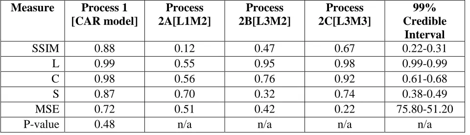
The Bayesian posterior predictive p-value revealed the posited model did fit the generated data, as the p-value based on the sample mean was 0.47 (where p-values in the tails indicate poor fit). When the average values for Yrep were compared with the observed values for each cell (i.e., a
pixel-by-pixel comparison), the mean square error was 0.72, for a dependent variable with mean 3.19 and standard deviation 2.31.
Figure 3 about here
Fig. 3 presents a map comparison analysis comparing the Yrep to the observed data. The
mean SSIM index score was 0.88, varying between 0.78 and 0.89 when comparisons were made between each of the 100 Yrep and Y. The SSIM index components mapped in Fig. 3 reveal that the
17 index. On the left side (Fig. 3a-d), a difference in pattern is highlighted by the S component as well, while the map of errors appear to have no spatial structure.
Space-time Model Assessment
The SSIM analysis results of the space-time models are outlined in Table 2. For the simplest case, with linear spatial trend and no temporal trend in translocation, the structural similarity was poorest, with a mean SSIM index of 0.12. The components responsible for this low score were L (0.55) and C (0.56), whereas S was higher (0.70). Conversely, for patterns generated from a GMRF exhibiting spatial non-stationarity (processes 2B and 2C), L (0.95, 0.98) and C (0.76, 0.92) scored higher, whereas S scored lower (0.32, 0.74). In all cases, the global SSIM index indicates differences in spatial structure between true model parameters and those estimated by the model. Of all models examined, process 2A had the lowest scores in the SSIM analysis. Threshold-like behaviour is evident, whereby values for λ below 1 could not be estimated accurately. Dependence between L and C is evident, as those areas that scored low in L had higher C scores. The S component was high due to the simple nature of the pattern (i.e., a linear vertical trend). The best fitting model spatially was for process 2C, with spatial nonstationarity for local spread and sinusoidal temporally random spread (Fig. 4). S and C were components dominating spatial estimation error in this more complex process. The small luminance errors were smoothed over by the moving window, yielding high L across the study area. Dashed areas in Fig. 4 highlight both S and C as contributing components. Interestingly, the high error hotspot evident in the map of squared errors is completely smoothed over in the SSIM maps. Because the smoothing is a function of the window size (5x5) and the smoothing function (none used here), SSIM results must be interpreted relative to these two parameters.
18 Figure 4 about here
A Case Study: Bayesian Kriging
The simulation study demonstrates the use of the SSIM index in a context in which we have a known value for a spatial variable, and we estimate a model, and we make comparisons.
However, practical spatial modelling encounters few situations where the true values of a spatial variable are known. Typically when building spatial models, the only data available to assess model fit are used to build a model. As discussed previously, posterior predictive checking provides a framework for using a model to draw new simulations from a posited process, and these can be compared with the original data. In this case, model assessment takes one of two forms: 1) check different realizations of spatial models against one thought to be the best, or 2) compare all iterations of models against each other. We employ the former strategy in an assessment of precipitation modelling in Sri Lanka.
The Study Area and Data
Sri Lanka is situated in the Indian Ocean, off the southeastern tip of the Indian subcontinent. The climate is tropical, and weather is characterized by two seasonal monsoons. The northeast (maha) monsoon typically lasts from October until March, whereas the southwest (yala)
19 Precipitation data were obtained from the Department of Meteorology of Sri Lanka. They include daily rainfall measurements (millimeters) from a network of 361 small-scale
agro-ecological weather monitoring stations (Fig. 5). The spatial distribution of the station network varies considerably with population, climate, and landuse. For this research, daily rainfall measurements were aggregated into total monthly rainfall. A subset of these data was extracted for the month of December 2008.
Figure 5 about here
Daily rainfall data were obtained from 20 official meteorological stations operated by the Department of Meteorology of Sri Lanka. This data set was aggregated into monthly rainfall for December 2008. The official meteorological station data (n = 20) was used to validate the interpolations generated using the larger (n = 361) agro-ecological monitoring data.
Methods
Bayesian kriging was used to interpolate rainfall values across Sri Lanka onto a regular spatial lattice (1 km grid cells). Bayesian kriging differs from ordinary kriging in that priors are put on parameters of the semivariogram, and estimation yields a posterior distribution for each of the parameters (range, sill, and nugget). Random draws from the posteriors were used to generate predictive simulations (i.e., Yrep) and these were compared to the simulation based on posterior
means using the SSIM index. Similar to the previous analysis, the variability expressed in the SSIM analysis reveals uncertainty in the fit of the predicted interpolations. A Gaussian spatial linear mixed model was used to perform Bayesian kriging. The R package geoR (Ribiero and Diggle 2001) was used to generate posterior predictive distributions. Because the initial rainfall values used to perform Bayesian kriging were not normally distributed, a Box-Cox
Box-20 Cox transformation searches for an exponent value which is applied to each observation in order to make the shape of the distribution more Normal. The interpolated data then were
back-transformed for analysis and interpretation. Posterior predictive simulations (n = 99) were obtained with kriging by using random draws from posterior distributions of the semivariogram parameters. Each interpolation was compared to the posterior mean interpolation using the SSIM index.
Results and Discussion
Fig. 6 presents a frequency distribution of mSSIM values from 99 Yrep compared to the posterior
mean. The majority of the mSSIM values were between 0.26 and 0.28. These values suggest that the interpolation generated from posterior predictive simulations were not very similar spatially to the posterior mean. The highest mSSIM value attained was 0.31, while the lowest was 0.22 (Table 2). Fig. 7 displays the SSIM map outputs attributed to both of these mSSIM values together with the posterior mean raster. While L was very high for both simulations (0.99), both C (high mSSIM: 0.68, low mSSIM: 0.61) and S (high mSSIM: 0.49, low mSSIM: 0.38) were notably lower, and can be thought to be responsible for the low mSSIM values. The spatial pattern of the distribution of rainfall in Sri Lanka is quite complex, which is reflected in the low S scores for both simulations.
Figure 6 about here
21 structural similarity in the southwest region of Sri Lanka (the most densely sampled area). This outcome suggests that the map of local SSIM index values is a much more important diagnostic tool in interpolation assessment than the global score.
Figure 7 about here
Appendix A summarizes a comparison of the observed rainfall measurements at the same 20 meteorological station locations to the predictions attained from the posterior mean from Bayesian kriging, as well as a variety of other different spatial interpolation methods (ordinary kriging, inverse distance weighting, and spline interpolation). While the mSSIM scores of comparisons between posterior predictive distribution simulations and the posterior mean interpolation were quite low, suggesting that visually, substantial change exists in model output in simulations from the posterior predictive distribution, Bayesian kriging attained the lowest mean absolute error (39.91 mm) over all 20 locations of any of the interpolation techniques.
Discussion
22 that look right. But we are not advocating the use of the SSIM index as a replacement for error based approaches; rather, we suggest that map comparison metrics should play a complimentary role in model assessment for spatial models. Fig. 1 highlights the need for this type of metric.
Two simulation experiments indicate that the SSIM index analysis provides additional information for model assessment purposes. However we have not defined any explicit criteria for distinguishing between good and bad model fit based on the SSIM index alone (e.g., SSIM index > 0.5 = good fit). The SSIM index, like many model assessment tools, is best used as a comparative measure of model agreement. The overall SSIM index is sensitive to three
components: L, C, and S, which are largely independent of each other. The SSIM index should be considered together with these three components, because each component provides unique information valuable for model assessment. Given that local SSIM index values are the product of local L, C, and S, a small SSIM index value may be the result of lower scores in all three components, or a mixture of high and low scores in various components. This relationship becomes further complicated as local values are averaged across a map to provide a global score. For example, comparing the individual component results from the space-time simulation
23 agreement. Such maps can be used to examine where and how well the spatial structure of model output matches some true map or expectation, and where that model fails.
Although the analysis here employs the SSIM index as the local spatial measure, this is by no means the only available option, and using this approach has its disadvantages. The SSIM index method is wholly dependent on the window size parameters (set here to a 5x5 local window on a 40x40 grid). Further, recently the whole notion of measuring perceived error using the SSIM has been questioned. Dosselmann and Yang (2011) suggest that the SSIM index is directly related to the MSE, and its formulation (a product of means, variances, and correlations) is too simple to actually model the human visual system. Regardless, while the mechanism accounting for its performance requires further investigation (e.g., luminance adaptation, textural masking), studies demonstrate its ability to accurately reflect subjective mean opinion scores (Wang et al. 2004). A major limitation in our application to maps is that the SSIM index method is implemented and tested only on maps defined using a regular spatial lattice, which currently limits its application in model checking to spatial models based on raster data or a regular square grid. Future work could explore the properties of this statistic for more complex spatial lattice structures; however in such cases, care must be taken in the definition of the spatial
24 SSIM index can be used in geographical analysis beyond relative comparisons. A final limitation is that the SSIM approach is scale dependent, and as in any pattern analysis, multiscale
approaches are critical to identify the scale sensitivity to observed patterns. This limitation is also true in the context of model assessment. Wavelet-based methods in particular may have potential for comparison of continuous valued maps, and thus spatial model assessment.
Conclusion
Typically, with spatial and space-time models, evaluation of model fit is based solely on traditional aspatial model diagnostics. Here we advocate for a spatially explicit approach to testing how some mapped spatial output from a model differs from an expectation as a
25
Table A1 Bayesian kriging predictions compared with multiple interpolation methods’ predictions and observed rainfall values at 20 official meteorological station locations
Observed Rainfall
(mm)
Bayesian Kriging
(mm)
Ordinary Kriging
(mm)
Inverse Distance Weighting
(mm)
Splines (mm)
259.57 265.65 242.57 305.78 355.68
96.52 110.76 117.77 102.21 104.02
146.71 130.85 127.61 137.72 27.24
160.92 195.28 143.87 129.11 109.91
91.31 115.82 82.94 81.25 87.58
251.81 182.12 150.87 143.18 -269.53
208.71 87.68 76.91 78.56 64.97
131.73 79.33 120.6 103.46 65.65
181.42 187.97 255.79 165.37 184.61
147.34 69.27 111.13 77.89 93.42
94.52 74.69 100.65 78.48 83.74
47.55 27.81 85.09 77.77 -56.74
304.12 254.76 206.55 280.13 302.9
57.34 35.59 58.62 39.55 42.44
276.23 312.12 206.95 277.32 281.86
321.94 256.53 251.12 216.97 273.74
313.3 283.09 198.65 282.93 352.18
244.92 294.18 235.45 206.31 215.22
166.84 171.85 123.34 46.63 -33.05
184.54 105.66 132.56 81.98 83.62
Average Absolute
27 Principle.” In Second International Symposium on Information Theory, 1:267–281. Springer
Verlag.
Anselin, L. (1988). Spatial Econometrics: Methods and Models. New York: Springer.
Anselin, L. (1995). “Local Indicators of Spatial association-LISA.” Geographical Analysis 27(2), 93–115.
Boots, B., and F. Csillag. (2006). “Categorical Maps, Comparisons, and Confidence.” Journal of Geographical Systems 8(2), 109–18.
Brunet, D., R. Vrscay, and Z. Wang. (2012). “On the Mathematical Properties of the Structural Similarity Index.” IEEE Transactions on Image Processing (99): 1488–1499.
Brundson, C., A.S. Fotheringham, and M. Charlton. (1996). “Geographically Weighted Regression: A Method for Exploring Spatial Nonstationarity.” Geographical Analysis 28(4),
281–98.
Burnham, K. P., and D. R. Anderson. (2002). Model Selection and Multi-model Inference: a Practical Information-theoretic Approach. New York: Springer.
28 Applications for Geographic Information Science and Technology. Thousand Oaks: SAGE.
Cliff, A., and J. K. Ord. (1981). Spatial Processes Models and Applications. London: Pion Limited.
Csillag, F., and B. Boots. (2005). “A Framework for Statistical Inferential Decisions in Spatial Pattern Analysis.” The Canadian Geographer 49(2), 172–79.
Dice L.R., (1945). “Measures of the Amount of Ecologic Association between Species.” Ecology 26(3), 297–302.
Ribeiro Jr., P.J. and P.J. Diggle. (2001). “geoR: A package for geostatistical analysis.” R-NEWS 1(2),15-18.
Dosselmann, R., and X. D. Yang. (2011). “A comprehensive assessment of the structural similarity index.” Signal, Image and Video Processing 5(1), 81–91.
Finley, A. O. (2011). “Comparing Spatially Varying Coefficients Models for Analysis of Ecological Data with Non Stationary and Anisotropic Residual Dependence.” Methods in
Ecology and Evolution 2(2), 143–54.
29 Gelfand, A. E., H.J. Kim, C. F. Sirmans, and S. Banerjee. (2003). “Spatial Modeling with
Spatially Varying Coefficient Processes.” Journal of the American Statistical Association
98(462), 387–96.
Gelman, A., and D. B. Rubin. (1992). “Inference from Iterative Simulation Using Multiple Sequences.” Statistical Science 7 (4), 457–72.
Gelman A, X.L. Meng XL, and H. Stern. (1996). “Posterior Predictive Assessment of Model Fitness via Realized Discrepancies.” Statistica Sinica 6,733–59.
Getis, A., and C. Ord. (1992). “The Analysis of Spatial Association by use of Distance
Statistics.” Geographical Analysis 24(3), 189–206.
Gong, P., and B. Xu. (2003). “Remote Sensing of Forests over Time: Change Types, Methods, and Opportunities.” In Remote Sensing of Forest Environments: Concepts and Case Studies, 301–34, edited by M.A. Wulder, and S.E. Franklin. Norwell: Kluwer Academic Publishers.
30 Linear Mixed Models: The MCMCglmm R Package.” Journal of Statistical Software 33(2), 1–
22.
Hagen-Zanker, A. (2006a). “Comparing Continuous Valued Raster Data: A Cross Disciplinary Literature Scan.” Netherlands Environmental Assessment Agency. Maastricht: Research Institute for Knowledge Systems.
Hagen-Zanker, A. (2006b). “Map Comparison Methods that Simultaneously Address Overlap and Structure.” Journal of Geographical Systems 8(2), 165–85.
Hagen-Zanker, A., and P. Martens. (2008). “Map Comparison Methods for Comprehensive Assessment of Geosimulation Models.” Lecture Notes in Computer Science 5072, 194–209.
Hagerstrand, T. (1953). “On Monte Carlo simulation of diffusion” in Economic and Cultural
Topics ( Quantitative Geography, Part I, edited by W L Garrison, D F Marble, [2 vols.;
Evanston, Illinois: Northwestern University Department of Geography, 1967]), 1-32.
Kass, R. E., and A. E. Raftery. (1995). “Bayes Factors.” Journal of the American Statistical
Association 90 (430), 773–795.
31 Lee, H., and S. K. Ghosh. 2009. “Performance of Information Criteria for Spatial Models.” Journal of Statistical Computation and Simulation 79 (1): 93–106.
Long, J. A., C. Robertson, F.S. Nathoo, and T.A. Nelson. (2012) “A Bayesian Space–time Model for Discrete Spread Processes on a Lattice. Spatial and Spatio-temporal Epidemiology 3, 151-162.
Lunn, D. J., A. Thomas, N. Best, and D. Spiegelhalter. (2000). “WinBUGS - A Bayesian
Modelling Framework: Concepts, Structure, and Extensibility.” Statistics and Computing 10 (4),
325–37.
Pontius Jr, R.G., (2000). “Quantification Error versus Location Error in Comparison of Categorical maps.” Photogrammetric Engineering and Remote Sensing 66,1011–16.
Räty, M., and A. Kangas. (2010). “Segmentation of Model Localization Sub-areas by Getis Statistics.” Silva Fenn 44 (2), 303–17.
Remmel, T., and F. Csillag. (2003). “When Are Two Landscape Pattern Indexes Significantly Different.” Journal of Geographical Systems 5, 331–51.
Schwarz, G. 1978. “Estimating the Dimension of a Model.” The Annals of Statistics 6 (2): 461–
32 Smith D.L., B. Lucey, L.A.Waller, J.E. Childs, and L.A. Real. (2002). “Predicting the Spatial Dynamics of Rabies Epidemics on Heterogeneous Landscapes.” Proceedings of the National Academy of Sciences 99, 3668–72.
Spiegelhalter, D. J., N. G. Best, B. P. Carlin, and A. Van Der Linde. (2002). “Bayesian Measures of Model Complexity and Fit.” Journal of the Royal Statistical Society: Series B (Statistical
Methodology) 64 (4): 583–639.
Turchin, P., and W. Thoeny. (1993). “Quantifying Dispersal of Southern Pine Beetles with Mark-recapture Experiments and a Diffusion Model.” Ecological Applications 3(1), 187–98.
Thomas, E. N. (1968). Maps of Residuals from Regression: Their Characteristics and Uses in Geographic Research. Ann Arbor: University Microfilms, A Xerox Company.
Visser, H., and T. de Nijs. (2006). “The Map Comparison Kit.” Environmental Modelling & Software 21(3), 346–58.
33 Assessment.” IEEE Transactions on Image Processing 20 (5), 1185–98.
Wheeler D.C., and L.A.Waller. (2008). “Mountains, Valleys, and Rivers: The Transmission of Raccoon Rabies over a Heterogeneous Landscape.” Journal of Agricultural, Biological, and Environmental Statistics 13, 388–406.
34
Name Model Parameters Spatial Parameter
[image:36.612.69.424.112.193.2]1 µ, σ σ – Exponential distance decay 2A Λ, M Λ – Linear vertically increasing 2B Λ, M Λ – Gaussian Markov Random Field 2C Λ, M Λ - Gaussian Markov Random Field
Table 2 Average SSIM index values, component values and MSE for 100 Y replicate data obtained from a conditional autoregressive model (Process 1) and three space-time models (process 2A, 2B, 2C). The range of SSIM index and component values obtained from a Bayesian kriging case study of spatial interpolation of rainfall in Sri Lanka (99% credible interval) .
[image:36.612.66.546.288.426.2]Measure Process 1 [CAR model]
Process 2A[L1M2]
Process 2B[L3M2]
Process 2C[L3M3]
99% Credible
Interval
SSIM 0.88 0.12 0.47 0.67 0.22-0.31
L 0.99 0.55 0.95 0.98 0.99-0.99
C 0.98 0.56 0.76 0.92 0.61-0.68
S 0.87 0.70 0.32 0.74 0.38-0.49
MSE 0.72 0.51 0.42 0.22 75.80-51.20
35 noise added. Distorted maps have similar mean squared errors (MSE) when compared with the reference map, but different SSIM index values.
Figure 2. An overview of the analysis methodology used in this paper, including simulation studies (a-b) and, c) a case study of rainfall interpolation in Sri Lanka.
Figure 3. Spatial model results comparing a reference map (observed data) with one replicate dataset simulated by a random draw from posterior distributions of model parameters (replicate data). The SSIM index, squared error, and SSIM components are presented. Dashed lines indicate areas of spatial discrepancy based on SSIM index analysis.
Figure 4. Space-time model results comparing a reference map (true λ) with posterior mean estimates for spatial diffusion parameters. The SSIM index, squared error, and SSIM
components are presented. Dashed lines indicate areas of spatial discrepancy based on SSIM index analysis.
Figure 5. Locations of official meteorological stations and small scale weather stations in Sri Lanka. 2008.
Figure 6. Histogram of mSSIM values from 99 simulations drawn from the posterior distribution.