1
Stated and revealed inequality aversion
in three subject pools
Benjamin Beranek
1, Robin Cubitt
1, Simon Gächter
1,2 1University of Nottingham
*,
2CESifo, IZA
25 March 2015Abstract. This paper reports data from three subject pools (n=717 subjects) using techniques based on those of Loewenstein, et al. (1989) and Blanco, et al. (2011) to obtain parameters, respectively, of stated and revealed inequality aversion. We provide a replication opportunity for those papers, with two innovations: (i) a design which allows stated and revealed preferences to be compared at the individual level; (ii) assessment of robustness of findings across subjects from a UK university, a Turkish university and Amazon Mechanical Turk. Our findings on stated aversion to inequality are qualitatively similar to those of Loewenstein, et al. in each of our subject pools, whereas there are notable differences between some of our findings on revealed preference and those of Blanco, et al. We find that revealed advantageous inequality aversion is often stronger than revealed dis-advantageous inequality aversion. In most subject pools, we find some (weak) correlation between corresponding parameters of stated and revealed inequality aversion.
Keywords: inequality aversion, replication, revealed and stated preferences, robustness across subject pools, MTurk.
JEL Classification Codes: C90
Acknowledgements
This paper is part of and funded by the research project ERC-AdG 295707 COOPERATION. We also acknowledge support from the ESRC funded Network for Integrated Behavioural Science (NIBS, ES/K002201/1).We received helpful comments from the editor, Nikos Nikiforakis, three referees, and from Abigail Barr, Dirk Engelmann, Lucas Molleman, Pawel Smietanka,Klaus Schmidt, Jonathan Schulz, Till Weber, Ori Weisel, and participants at the ESA conference in Prague and a seminar at the University of Nottingham. We are grateful to Mariana Blanco, Dirk Engelmann and Hans Normann for providing us with the data, zTree code and instructions from Blanco, et al. (2011).
*
Centre for Decision Research and Experimental Economics, School of Economics, Sir Clive Granger Building, University Park, Nottingham NG7 2RD.
2
1. Introduction
Inequality aversion, the dislike of unequal outcomes, has become established as one of
the core postulates of behavioural economics. Although discussion of equity concerns is by
no means new (e.g., Adams 1965; Selten 1978), the recent literature took off with publication
of formal models of inequality averse preferences by Bolton (1991), Bolton and Ockenfels
(2000) and Fehr and Schmidt (1999), with the latter paper providing the most widely applied
model. In this paper, we are concerned with the range of empirically relevant parameters of
inequality aversion. We concentrate on aversion to inequality in bilateral monetary
comparisons, as in Fehr and Schmidt’s theory.
To our knowledge, Loewenstein, et al. (1989) is the first paper to provide systematic
evidence on this. They presented their subjects with (hypothetical) life-like scenarios that
involved distributions of money between the subject and a comparator and asked the subjects
to rate their satisfaction with those distributions. We refer to these measurements as stated
preferences because they do not involve choices, but un-incentivized assessments of
satisfaction. On the basis of these ratings, Loewenstein, et al. estimated ‘social utility
functions’ and found that subjects dislike inequality when it is to their advantage and when it
is to their disadvantage. However, aversion to disadvantageous inequality was considerably
stronger than aversion to advantageous inequality. Fehr and Schmidt use this observation
(pp. 821, 823-4) to justify their distinctive assumption that disadvantageous inequality
aversion (measured in their model by a parameter called α) is at least as strong as
advantageous inequality aversion (measured by a parameter called β). A key subsequent step
taken by Blanco, et al. (2011) was to provide individual-level measures of α and β,
respectively, by using subjects’ choices in two particular games. Thus, importantly, their
3 In this paper, we replicate the Loewenstein, et al. experiments using updated versions of
their scenarios to elicit social utility functions; and we replicate Blanco, et al.’s measurement
of α and β using their games and procedures.1 In the latter case, like Blanco, et al., we will observe the joint distribution of α and β and so be able to reassess the extent to which elicited
values are consistent with Fehr and Schmidt’s assumption that α ≥ β. However, our most
novel contribution is that we link stated and revealed inequality aversion at the individual
level: for each subject, our experimental design yields parameters of stated disadvantageous
and advantageous inequality aversion obtained with methods akin to those of Loewenstein, et
al., and values of α and β revealed by choices using Blanco, et al.’s methods. As they refer to
the same inequalities but are obtained with different methods, we use a and b to denote the
stated preference analogues of α and β, respectively.
If inequality aversion is a general sentiment triggered across different situations, then
stated and revealed measures should be positively correlated across individuals. If they are,
measurements of stated and revealed preferences cross-validate each other. If they are not,
this would call into question how strongly the findings of Loewenstein, et al. could support
the modelling assumptions of Fehr and Schmidt.
We also investigate the association between inequality aversion and proneness to guilt,
which we measure using the GASP (guilt and shame proneness) scale of Cohen, et al. (2011).
This is particularly relevant to aversion to advantageous inequality, the parameter of which
(here b or β) is often referred to as the “guilt” parameter (e.g., Blanco, et al., p. 322).
Our data are from three subject pools, two of them drawn from the student bodies of the
University of Nottingham (UK) and Izmir University of Economics (Turkey) and the third
1
4 from the American online workforce of Amazon Mechanical Turk (MTurk).2 Across all subject pools, 717 people participated in our experiments. Apart from differences pertaining
to the subject pools, the experimental procedures were essentially uniform.
Our main results are as follows. Notwithstanding some differences in intensity, stated
inequality averse preferences are qualitatively similar in all three subject pools in that, like
Loewenstein, et al., we find that a ≥ b and b ≥ 0 for most subjects. This provides strong
support for the findings of Loewenstein, et al. that inspired Fehr and Schmidt’s theory.
However, the support for some aspects of that theory itself is weaker, as we find violations at
the individual and the median level in all subject pools of the assumption that α ≥ β. We find
only weak positive correlation between a and α. Correlation between b and β is significantly
positive and exceeds that for a and α in all subject pools. We find females are more averse
than males to advantageous inequality and that there is an association between inequality
aversion and the GASP measure of proneness to guilt and shame. Although there are some
differences between our findings from different subject pools, they are mostly not important
for central tendencies of parameters, especially once other factors are controlled for.
2. Methods
For brevity, we focus in this section on the main features of our experimental designs,
relegating technical and procedural details, instructions and scenario texts to the online
supplementary materials. Each subject completed all of the game tasks described in this
section, a selection of scenario tasks, the GASP task and some other tasks with no feedback
until all tasks had been completed. We describe the games here in terms of “points”, as we
did to subjects. At the end of the experiment, points from one game were converted to cash.
2
5 The core of this study is the two-person version of the Fehr and Schmidt (1999) model of
inequality aversion:
𝑈�=𝑥�− 𝛼�max�𝑥�− 𝑥�, 0� − 𝛽�max�𝑥�− 𝑥�, 0�,𝑗 ≠ 𝑖, 𝛼�≥ 𝛽�; 1 >𝛽� ≥0. (1)
In this functional form, 𝑈� denotes person i’s utility, 𝑥� person i’s monetary payoff and 𝑥�
the other person’s monetary payoff. The parameter 𝛼�governs i’s disutility from
disadvantageous inequality, i.e. from 𝑥� falling short of 𝑥�; and the parameter 𝛽� governs i’s
disutility from advantageous inequality, i.e. from 𝑥� exceeding 𝑥�. A core assumption of Fehr
and Schmidt is that advantageous inequality has less of a negative impact on overall utility
than disadvantageous inequality of the same magnitude, i.e. 𝛼� ≥ 𝛽�. A central goal of our paper is to provide fresh estimates of the joint distribution of αi and 𝛽�.
A subject’s parameter 𝛽� of advantageous inequality aversion is elicited using a Modified Dictator game that Blanco, et al. introduced and which we implement in the same way. The
dictator has to make 21 decisions, each a choice between the distribution (20 points for self, 0
points for other) and an equal distribution (x points for self, x points for other), where “other”
refers to a passive player. The equal distributions increased in increments of 1 point from (0,
0) to (20, 20) in the obvious notation. As explained by Blanco, et al. (p. 325-326), the
dictator’s 𝛽� parameter is theoretically determined by the equal distribution (𝑥��, 𝑥��) which he regards as good as the distribution (20, 0). From equation (1), 𝑈�(20, 0) = 𝑈�(𝑥��, 𝑥��) if, and only if, 20−20𝛽�=𝑥��. Thus,
𝛽� = 1−����� .
Following Blanco, et al., we assume that, as x rises in steps, subjects will switch (once) from
6 chosen. 𝛽� = 1 (resp. 0) is assigned to a subject who always (resp. never) chooses the equal option.
Following Blanco, et al. (p. 325) (and in line with a suggestion of Fehr and Schmidt)
behavior in the Ultimatum game of Güth, et al. (1982) can be used to elicit the parameter αi of
revealed disadvantageous inequality aversion. One player (the proposer) proposes to the
other player (the responder) an allocation of a fixed sum (here of 20 points). Then, the
responder chooses between accepting the proposal and rejecting it. In the former case, the
proposal is implemented; but, in the latter case, both participants receive 0 points. All
subjects make decisions in both roles, using the strategy method for the responder’s decision,
so as to provide a response to all distributions that might be proposed.
A subject’s strategy in the role of responder yields an estimate of their 𝛼�parameter.
This is determined theoretically by the proposal 𝑠̃� at which the responder is just indifferent between accepting and rejecting. From (1), 𝑈�(𝑠̃�, 20− 𝑠̃�) = 𝑠̃�− 𝛼�(20− 𝑠̃�− 𝑠̃�) = 0 determines the point of indifference, and thus,
𝛼� =�(����̃�̃� �).
Following Blanco, et al., when there is no more than one switch-point in the responder’s
strategy, we approximate 𝑠̃� with the average of the lowest accepted offer and the highest rejected offer. Subjects who do not reject any offers are assigned 𝛼� = 0 and those who reject all offers less favorable to them than an equal split are assigned 𝛼� = 4.5 (Blanco, et al., p. 325).
7 switched multiple times in either of these sequences, and is thus not well behaved, is
excluded from the data reported in Section 3.
We turn now to the elicitation of stated preferences. In Studies 1 & 2 of Loewenstein,
et al. (1989), participants read various scenarios describing a range of possible distributions
of outcomes, with the subject in the role of one of the affected parties in a bilateral dispute.
Subjects ranked their satisfaction of outcomes on an 11-point scale. In our study, we follow
the design of Loewenstein, et al., but use modernized scenario tasks. This part of the design is
2×2×2, varying the nature of the issue disputed (distributing the proceeds of an invention or
of a plot of land between two parties), the prior relationship between the two parties (positive
or negative), and whether it is gains or losses which are to be distributed. Thus, in total there
are eight different scenarios. For each one, the task is to rate 21 distributions of payoffs for
the subject and the other person described in the scenario. Each subject was presented with
four different scenarios. For each subject, the resulting 84 ratings are used to estimate a
“social utility” function of the same form as (1) (plus the addition of a constant) to obtain
estimates of their stated advantageous and disadvantageous inequality aversion parameters
(called ai and bi). The estimation used OLS, with the subject’s stated satisfaction as the
dependent variable. By construction, this procedure produces a value of ai and a value of bi
for each subject but, as explained above, subjects with non-well-behaved revealed
preferences are excluded from Section 3. This guarantees that the revealed and stated
preferences reported are drawn from the same set of subjects.
Though we may expect positive rank correlation across individuals between 𝑎� and 𝛼� (resp. between 𝑏� and 𝛽�) if inequality aversion is a general sentiment across domains, the presence of such correlation is certainly not built in to the design. The scenario tasks and the
8 response modes are not the same, and the contexts described in the scenarios differ from
those posed by the game instructions.
We are interested in the generalizability across subject pools of the findings on stated
and revealed inequality aversion. Replication in a culturally different society and outside the
university environment is important because there is mounting evidence that student subjects
from European or North American universities often are quite special, when compared to
others (Henrich, et al. 2010; Barr, et al. 2009; Herrmann, et al. 2008).
We conducted sessions at the University of Nottingham (n=104 students, all British);
at Izmir University of Economics (n=206 students, all Turkish); and on the MTurk platform
(n= 407 adult residents of the US). Culturally, there is significant distance between the UK
and Turkey; and the MTurk sample differs from both university samples, especially by
having greater variety of ages and education levels, and by being American.
In both university samples, the experiment was programmed in zTree (Fischbacher 2007)
using, in the case of the games, zTree code and instructions provided by Blanco, et al.. In
Nottingham, recruitment was done using ORSEE (Greiner 2004). In Izmir, recruiting
required approaching students on campus. The MTurk experiments were conducted using the
online survey software Qualtrics and the MTurk platform. In all cases, the experiments were
followed by post-experimental questionnaires, which elicited socio-demographic information,
as well as the measure of guilt and shame proneness (Cohen, et al. 2011).
3. Results
3.1. Stated inequality aversion
Our first result concerns the ai and bi parameters of stated inequality aversion derived
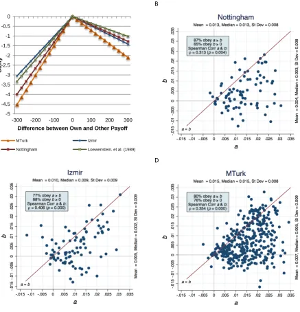
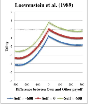
9 and bi parameters across each subject pool (and normalizing the constant to zero). Fig. 1A
shows averaged utility as a function of the difference between Own and Others payoff, when
one’s own payoff is zero. In all three of our subject pools, averaged utility is positively
sloped in the region of disadvantageous inequality (to the left of zero on the horizontal axis)
and negatively sloped in the region of advantageous inequality. Also, in all three of our
subject pools and in line with Loewenstein, et al., the slope of averaged utility is greater in
absolute value in the former region than in the latter, implying that disadvantageous
inequality had a greater negative impact on satisfaction ratings than the corresponding
advantageous inequality.
Fig. 1A also shows that, especially in the region of advantageous inequality, the averaged
social utility curves of the Nottingham and Izmir subject pools are quite similar to one
another and to corresponding curves from the Loewenstein, et al. findings (see online
materials). In contrast, the averaged social utility curves from the MTurk sample show more
pronounced aversion to both forms of inequality. Kruskal-Wallis tests confirm that there are
statistically significant differences between our subject pools in bivalues (χ2(2)=8.779,
p=0.0124) and, especially, in aivalues (χ2(2)=23.858, p<0.001), an issue to which we return
in Section 3.4.
FIGURES 1A- 1D
Figs. 1B to 1D illustrate the joint ai and bi distributions for each of our subject pools.
Recall that a key assumption of Fehr and Schmidt is that 𝛼�≥ 𝛽� which they justify referring to the Loewenstein, et al results. In our notation, the corresponding finding to that of
Loewenstein, et al. would be tendency for ai to exceed bi. We find strong support for this, as
ai≥ bi for 87%, 77%, and 80% of participants in the Nottingham, Izmir, and MTurk subject
10 violate the condition bi≥ 0, so displaying a stated preference for advantageous inequality.
This finding is consistent with observation of the existence of spiteful preferences in related
literature (e.g., Balafoutas et al., 2012; Iriberri and Rey-Biel, 2013).
Figures 1B–1D also report that ai and bi are positively correlated across individuals in
each subject pool. In the pooled data, the corresponding Spearman rho is 0.3784 (p<0.0001).
3.2. Revealed inequality aversion
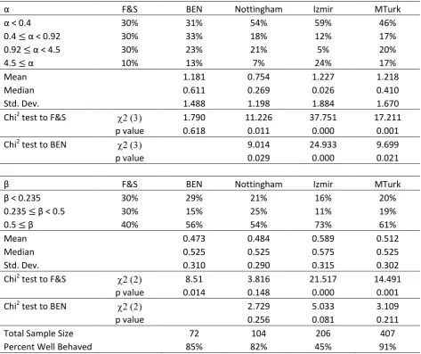
Table 1 shows the distribution of 𝛼� (top panel) and 𝛽� (lower panel) for each subject pool, using the categories of Blanco, et al.’s Table 2. We compare our observed distributions
to Blanco, et al.’s interpretation (p. 326) of the distribution which Fehr and Schmidt deem
plausible and to the distributions which Blanco, et al. themselves observe. Table 1 reports the
relevant Chi2-tests in each case, as well as the mean, median and standard deviation of each parameter in each subject pool.
TABLE 1
The upper panel of Table 1 reveals that, in all three of our subject pools, values of αi in
the range of αi < 0.4 are substantially more frequent than in the Blanco, et al. data (between
46% and 59% of our subjects have an αi < 0.4, compared to 31% in Blanco, et al.). Values of
αi≥ 4.5 are, with the exception of Nottingham, also more frequent in our subject pools than in
the Blanco, et al. data (7%, 24%, and 17%, in Nottingham, Izmir, and MTurk, respectively,
compared to 13% in Blanco, et al.). Chi2-tests confirm thatall three of our subject pools differ significantly (at p=0.03 or lower) in respect of αi from both the Fehr and Schmidt and the
Blanco, et al. distributions of this parameter.
11 in our Nottingham and MTurk samples (p=0.26 and 0.21, respectively), and only a weakly
significant difference in the Izmir sample (p=0.08). Comparing our distributions to those
assumed by Fehr and Schmidt, using Chi2-tests, reveals significantly different distributions in the Izmir and MTurk sample (p<0.01), but an insignificant difference between the
Fehr-Schmidt distribution and that of our Nottingham sample (p=0.15).
Our next result concerns Fehr and Schmidt’s assumption that 𝛼� ≥ 𝛽�. A first, aggregate level, take is provided by comparing the means and medians documented in Table 1. We find
that the mean value of αi is indeed larger than the mean 𝛽� in all our subject pools (as in
Blanco, et al.). However, the median αi is lower than the median 𝛽� in all our subject pools
(unlike in Blanco, et al.).
Table 1 also shows notable variation in the percent of 'well-behaved' participants (as
defined above) in each subject pool. In the Blanco, et al. subject pool, 85% of participants
were well-behaved. Our Nottingham and MTurk subject pools displayed similar percentages
of well-behaved participants (82% and 90% respectively), but only 45% of our Izmir sample
met the criteria of well-behavedness.
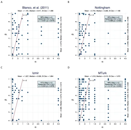
The four panels of Fig. 2 give the joint (αi, 𝛽�) distributions for the Blanco, et al. subject
pool and for each of our subject pools. As was foreshadowed in the medians, we see many
violations of the assumption that αi≥𝛽� in our subject pools. Whereas Blanco, et al. reported
38% of their participants violating this assumption, we find55%, 59%, and 51% of
participants violating it in Nottingham, Izmir, and MTurk, respectively. Like Blanco, et al.,
we also find that αi and 𝛽� are uncorrelated in Nottingham and Izmir; in the MTurk sample
the correlation between αi and 𝛽� is slightly (but significantly) negative. In the pooled data,
the correlation is very slightly negative (rho = - 0.089; p=0.038).
12 3.3 Relationship between stated and revealed preferences
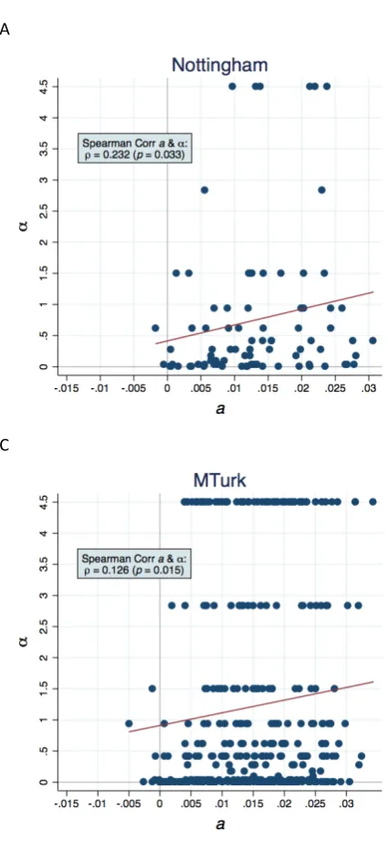
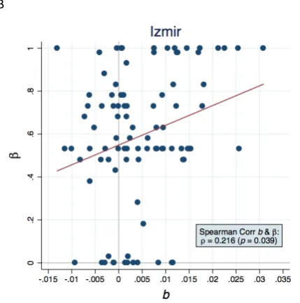
Fig. 3 shows the joint distribution of 𝑎� (stated) and 𝛼�(revealed) parameters of disadvantageous inequality aversion for each subject pool, with the associated Spearman’s
rho and its significance level. Surprisingly, there is no significant correlation between 𝑎� and 𝛼� in the Izmir pool; and, though the correlation is statistically significant in the other two
pools, it is only rather weakly positive, especially in the MTurk sample. In the pooled data,
the correlation is slightly positive (rho = 0.132; p=0.002).
FIGURE 3
The corresponding materials for the joint distribution of 𝑏� (stated) and 𝛽� (revealed) parameters of advantageous inequality aversion are shown in Fig. 4. For these parameters,
the correlation is positive and statistically significant in all three subject pools. The degree of
correlation is still quite modest, but higher in each subject pool than for 𝑎� and 𝛼�. In the pooled data, the correlation is moderately positive (rho = 0.2785; p<0.001).
FIGURE 4
3.4 The role of socio-demographics and guilt proneness for inequality aversion
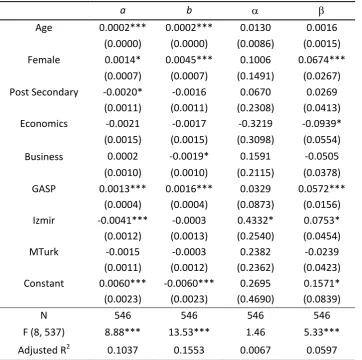
Finally, we pool the data from all three subject pools and separately regress our four
measures of inequality aversion (ai, bi, αi, βi) on three standard socio-demographic variables –
namely age, a female dummy, and a dummy for having some post-secondary education – and
on a dummy for having studied Economics or Business, the GASP scale, and on dummies for
Izmir and MTurk (the Nottingham subject pool being the omitted category). Across all our
subject pools there is considerable age variation (18-75 years), largely due to the MTurk
population. Between 41% and 46% of participants were females, across the three subject
post-13 secondary education status, with 5% having studied Economics and 12% Business. Table 2
records the results of the regressions.
TABLE 2
Age is a significant predictor of stated inequality aversion of both forms, but not of the
corresponding revealed preference parameters. Compared with males, females state slightly
stronger aversion to disadvantageous inequality aversion, but show significantly higher
estimates for stated and revealed advantageous inequality aversion. This result is consistent
with the experimental evidence that females give more than men in dictator games (e.g.,
Eckel and Grossman 1998; Engel 2011). Participants who had studied either Economics or
Business showed marginally significantly lower aversion to advantageous inequality (for
Economics in revealed preference but for Business in stated preference). Finally, with the
exception of αi, all inequality aversion parameters are highly significantly positively
correlated with GASP (higher scores indicate a greater proneness towards guilt and shame).
The remaining subject pool difference that stands out once all these factors are controlled for
is that Izmir subjects have significantly lower values of 𝑎�.
4. Discussion and conclusion
In terms of replication, our main results are as follows. The qualitative findings of
Loewenstein, et al. appear rather robust in that the central tendencies of our stated preference
data, in each subject pool, support the hypothesis of aversion to advantageous and
disadvantageous inequality, with the latter the more keenly felt. Thus, these findings
reinforce one of the main ingredients of Fehr and Schmidt’s motivation for their model. In
14 Fehr and Schmidt’s model and to the findings of Blanco, et al., whose revealed preference
techniques we use. We find widespread violation of Fehr and Schmidt’s assumption that αi≥
𝛽�. Although our results on the distribution of the parameter 𝛽� of aversion to advantageous
inequality are similar to the corresponding findings of Blanco, et al., our distributions of the
parameter 𝛼� of disadvantageous inequality aversion that differ markedly from that observed by Blanco, et al. Compared with them, we find a notably larger proportion of low values of
the parameter in all of our subject pools; and also a larger proportion of high values of the
parameter, in particular in our Izmir sample.
Below, we comment further on two of our most striking findings - weak correlation
between stated and revealed preferences and the frequent violation of Fehr and Schmidt’s
assumption that αi≥ 𝛽�, just mentioned – and on differences between our subject pools.
We observe statistically significant positive rank correlations across individuals between
(stated) 𝑏� and (revealed) 𝛽� parameters of advantageous inequality aversion in all three of our subject pools; and between (stated) 𝑎� and (revealed) 𝛼� parameters of disadvantageous inequality aversion in two of those pools.3 But, in all six cases, Spearman’s rho was below 0.32, suggesting only a weak relationship. We can think of three possible reactions to this.
One perspective (provided by a referee) is that difference between stated and revealed
preferences is an indication of “hypothetical bias” in the former, arising perhaps because
subjects do not take un-incentivized tasks seriously or use them to indulge in cheap talk. A
second perspective (provided by another referee) is that the difference between stated and
revealed preferences, combined with greater conformity of the former to theoretical
predictions, indicates that the scenario tasks “work” better, perhaps because subjects find
3
It is interesting that the correlation is stronger between the “pro-social” parameters 𝛽� and bi. Studies which
15 them more recognizable or accessible than the stripped-down lab games. A third perspective
is that the scenario tasks and the laboratory games both “work”, but they measure slightly
different things - in one case, an attitude and, in the other case, willingness to take a certain
kind of action. These are correlated because there is an underlying propensity to act on ones
attitudes. But, the correlation need not be strong, for example if the propensity to act on ones
attitudes is itself a trait whose strength varies across individuals.
To elaborate, the satisfaction ratings of the scenario tasks may indicate subjects’
happiness with (or feelings about) different outcomes, whereas the Modified Dictator and
Ultimatum games indicate subjects’ willingness to sacrifice monetary payoffs in order to
change the payoff of the other player in the game. This perspective chimes with the
discussion of Blanco, et al. (Section 7) of their finding that the Fehr-Schmidt model, taken
with parameter values elicited with their revealed preference methods, predicts the play of
games other than those used in the elicitation less successfully at the individual level than at
the aggregate level. They point out that willingness to give up money in order to change the
other players’ payoff may be sensitive to the nature of the game, as well as to the type of
inequality faced.
These considerations are also relevant to our findings about the relative strength of
aversion to advantageous and disadvantageous inequality. Even if adherence to some ethical
codes might induce the opposite attitude, we would expect most subjects to be happier on
receiving the larger part of some given unequal allocation between two people than on when
receiving the smaller part. If the satisfaction ratings of our scenario tasks are indicators of
happiness, in this sense, then our stated preference findings strongly support this expectation.
In contrast, our finding that a majority of subjects violate the assumption that αi≥ 𝛽� is a
matter of revealed preferences. Viewed more narrowly, it is a matter of the trade-offs that
16 A subject assigned a low value of 𝛼� is one who is reluctant to leave positive offers on the table when playing as respondent in the Ultimatum game. We report more instances of
this than most previous studies, but reluctance to leave money on the table is not completely
counter-intuitive behavior, even for a subject who feels unhappy about getting less than the
proposer. And, of course, homo economicus has αi = 0.
In the Modified Dictator game with which 𝛽� is elicited, our findings are comparable with those of Blanco, et al.. Mean values of around 0.5 seem quite high (especially relative
to homo economicus), but the discussion of Blanco, et al. (p. 333) suggests a possible reason
for this shared finding. The active player may feel responsible for the passive player in the
Modified Dictator game; and looking out for that player’s interests would tend to boost the
elicited value of 𝛽�, even for a subject who would not put much weight on the payoff of another in different circumstances.
These arguments suggest that, taken on its own, a finding that some individual violates αi
≥ 𝛽� may not be all that surprising, when one keeps in mind that the condition is on revealed
preference. Nevertheless, we find more frequent violations than Blanco, et al. had, and this
was contrary to our expectations. Further studies would be useful, especially in non-standard
subject pools.
That said, the similarities between our findings from distinct subject pools are arguably
more striking than the differences, with two exceptions each of which relates to revealed
preference. The first is the much greater incidence of non-well-behaved responses to the
revealed preference tasks in Izmir than in the other two subject pools. The second is greater
incidence among well-behaved subjects of extreme values (high and low) of 𝛼� among the Izmir subject pool, as compared with Nottingham and MTurk. One possible interpretation of
17 But, we cannot rule out some more fundamental, society-related subject-pool differences (a
possibility suggested by Herrmann, et al. 2008).
There is nothing inherently puzzling about one society displaying more extreme values
of revealed aversion to disadvantageous inequality than another, especially as this aversion is
inferred from the subject’s strategy as responder in the Ultimatum game. It may be that, in
some societies, there is a strong motivation not to leave money on the table, but this can be
over-ridden by a sense of insult and, if it is, then the opposite reaction is also powerful. As
Blanco, et al. (Section 7) notes, the Fehr-Schmidt model can be re-interpreted as an indirect
reduced-form for reciprocal motivations. Such motivations could affect the aversion to
disadvantageous inequality that we infer from the responder’s strategy in the Ultimatum
game. Thus, a possible explanation of differences between subject pools in this parameter is
that they differ either in the strength of their reciprocity or in the consistency across
individuals of how they balance reciprocal concerns with pure aversion to inequality.
The interpretation of the Fehr-Schmidt model as a reduced-form for reciprocal
motivations is also relevant to points discussed earlier. If the mapping between material
inequality and reciprocity is sensitive to context, that might contribute to the weak association
which we find between stated and revealed aversion to disadvantageous inequality. To the
extent that positive and negative reciprocity are distinct motivations (as is suggested by
existing evidence from related ultimatum and dictator games, e.g., Yamagishi, et al. 2012;
Peysakhovich, et al. 2014), this perspective would also help to explain why positive and
negative inequality aversion, as revealed in the Blanco, et al. tasks are not strongly positively
18
References
Adams, J. S. (1965). Inequity in social exchange. New York: Academic Press.
Balafoutas, L., Kerschbamer, R., & Sutter, M. (2012). Distributional preferences and competitive behavior. Journal of Economic Behavior & Organization, 83, 125-135.
Barr, A., Wallace, C., Ensminger, J., Henrich, J., Barrett, C., Bolyanatz, A., Cardenas, J. C., Gurven, M., Gwako, E., Lesorogol, C., Marlowe, F., Mcelreath, R., Tracer, D., & Ziker, J. (2009). Homo aequalis: A cross-society experimental analysis of three bargaining games. Oxford University Department of Economics Discussion Paper 422.
Blanco, M., Engelmann, D., & Normann, H. T. (2011). A within-subject analysis of other-regarding preferences. Games and Economic Behavior, 72, 321-338.
Bolton, G. E. (1991). A comparative model of bargaining - theory and evidence. American Economic Review, 81, 1096-1136.
Bolton, G. E., & Ockenfels, A. (2000). ERC: A theory of equity, reciprocity, and competition. American Economic Review, 90, 166-93.
Chandler, J., Mueller, P., & Paolacci, G. (2014). Nonnaïveté among amazon mechanical turk workers: Consequences and solutions for behavioral researchers. Behavior Research Methods, 46, 112-130.
Cohen, T. R., Wolf, S. T., Panter, A. T., & Insko, C. A. (2011). Introducing the GASP scale: A new measure of guilt and shame proneness. Journal of Personality and Social Psychology, 100, 947-966.
Dannenberg, A., Riechmann, T., Sturm, B., & Vogt, C. (2007). Inequity aversion and individual behavior in public good games: An experimental investigation. ZEW Discussion Paper 07-034. Dannenberg, A., Riechmann, T., Sturm, B., & Vogt, C. (2012). Inequality aversion and the house
money effect. Experimental Economics, 15, 460-484.
Dariel, A., & Nikiforakis, N. (2014). Cooperators and reciprocators: A within-subject analysis of pro-social behavior. Economics Letters, 122, 163-166.
Eckel, C., & Grossman, P. (1998). Are women less selfish than men?: Evidence from dictator games. The Economic Journal, 108, 726-735.
Engel, C. (2011). Dictator games: A meta study. Experimental Economics, 14, 583-610.
Fehr, E., & Schmidt, K. M. (1999). A theory of fairness, competition, and cooperation. Quarterly Journal of Economics, 114, 817-68.
Fischbacher, U. (2007). Z-tree: Zurich toolbox for readymade economic experiments. Experimental Economics, 10, 171-178.
Greiner, B. (2004). An online recruitment system for economic experiments. In Forschung und wissenschaftliches Rechnen GWDG Bericht 63, ed. K. Kremer, & V. Macho. Göttingen: Gesellschaft für Wissenschaftliche Datenverarbeitung.
Güth, W., Schmittberger, R., & Schwarze, B. (1982). An experimental analysis of ultimatum bargaining. Journal of Economic Behavior and Organization, 3, 367-88.
Henrich, J., Heine, S. J., & Norenzayan, A. (2010). The weirdest people in the world? Behavioral and Brain Sciences, 33, 61-83.
Herrmann, B., Thöni, C., & Gächter, S. (2008). Antisocial punishment across societies. Science, 319, 1362-1367.
Horton, J. J., Rand, D. G., & Zeckhauser, R. J. (2011). The online laboratory: Conducting experiments in a real labor market. Experimental Economics, 14, 399-425.
Iriberri, N., & Rey-Biel, P. (2013). Elicited beliefs and social information in modified dictator games: What do dictators believe other dictators do? Quantitative Economics, 4, 515-547.
Loewenstein, G., Thompson, L., & Bazerman, M. (1989). Social utility and decision making in interpersonal contexts. Journal of Personality and Social Psychology, 57, 426-441.
Peysakhovich, A., Nowak, M. A., & Rand, D. G. (2014). Humans display a ‘cooperative phenotype’ that is domain general and temporally stable. Nature Communications, 5,
doi:10.1038/ncomms5939.
19
Teyssier, S. (2012). Inequity and risk aversion in sequential public good games. Public Choice, 151, 91-119.
Yamagishi, T., Horita, Y., Mifune, N., Hashimoto, H., Li, Y., Shinada, M., Miura, A., Inukai, K., Takagishi, H., & Simunovic, D. (2012). Rejection of unfair offers in the ultimatum game is no evidence of strong reciprocity. Proceedings of the National Academy of Sciences, 109, 20364-20368.
20 Figure 1. Stated Preferences on Aggregate and Individual Levels. Fig. 1A. Utility (satisfaction ratings) as a function of difference between own and other payoff in the scenario tasks. Figs. 1B to 1D. Joint a and b distributions per subject pool. Each dot represents a participant’s a and b parameters as calculated from their stated preferences in the updated Loewenstein, et al (1989) scenario tasks. (The corresponding individual level data for Loewenstein, et. al. are not available.) Observations to the left of the 𝑎=𝑏 line have 𝑎<𝑏.
A
C
B
D
-5 -4.5 -4 -3.5 -3 -2.5 -2 -1.5 -1 -0.5 0
-300 -200 -100 0 100 200 300
U
ti
li
ty
Difference between Own and Other Payoff
MTurk Izmir
[image:20.595.80.518.244.699.2]21 Table 1. Distribution of 𝜶 and 𝜷 values. BEN refers to the Blanco, et al. (2011) observed distribution and F&S to Fehr & Schmidt. The data in these two columns and the row classifications are reproduced from Blanco, et al. (p. 325). Percent Well Behaved includes participants who had at most one switching point in the Ultimatum Game and at most one switching point in the Modified Dictator game. Only these participants are included in the analysis of this paper; all others are excluded.
α F&S BEN Nottingham Izmir MTurk
α < 0.4 30% 31% 54% 59% 46%
0.4 ≤α < 0.92 30% 33% 18% 12% 17%
0.92 ≤α < 4.5 30% 23% 21% 5% 20%
4.5 ≤α 10% 13% 7% 24% 17%
Mean 1.181 0.754 1.227 1.218
Median 0.611 0.269 0.026 0.410
Std. Dev. 1.488 1.198 1.884 1.670
Chi2 test to F&S χ2 (3) 1.790 11.226 37.751 17.211
p value 0.618 0.011 0.000 0.001
Chi2 test to BEN χ2 (3) 9.014 24.933 9.699
p value 0.029 0.000 0.021
β F&S BEN Nottingham Izmir MTurk
β < 0.235 30% 29% 21% 16% 20%
0.235 ≤β < 0.5 30% 15% 25% 11% 19%
0.5 ≤β 40% 56% 54% 73% 61%
Mean 0.473 0.484 0.589 0.512
Median 0.525 0.525 0.575 0.525
Std. Dev. 0.310 0.290 0.315 0.302
Chi2 test to F&S χ2 (2) 8.51 3.816 21.517 14.491
p value 0.014 0.148 0.000 0.001
Chi2 test to BEN χ2 (2) 2.729 5.033 3.109
p value 0.256 0.081 0.211
Total Sample Size 72 104 206 407
22 Figure 2. Joint 𝜶 and 𝜷 Distributions. Each dot represents a participant’s 𝛼 and 𝛽 parameters as calculated from their revealed preferences in the Blanco, et al (2011) games. Observations to the left of the 𝛼=𝛽 line have 𝛼<𝛽 which violates the Fehr and Schmidt (1999) assumption.
A B
23 Figure 3. Joint 𝒂 and 𝜶 Distributions. Each dot represents a participant’s 𝑎 as calculated from their stated preferences and 𝛼 parameters as calculated from their revealed preferences. The line results from the linear regression of 𝛼 on𝑎.
A B
24 Figure 4. Joint 𝒃 and 𝜷 Distributions. Each dot represents a participant’s 𝑏 as calculated from their stated preferences and 𝛽 parameters as calculated from their revealed preferences. The line results from the linear regression of 𝛽 on𝑏.
A B
25 Table 2. OLS regression analysis of demographic and psychological determinants of stated and
revealed parameters of inequality aversion.
a b α β
Age 0.0002*** 0.0002*** 0.0130 0.0016 (0.0000) (0.0000) (0.0086) (0.0015) Female 0.0014* 0.0045*** 0.1006 0.0674***
(0.0007) (0.0007) (0.1491) (0.0267) Post Secondary -0.0020* -0.0016 0.0670 0.0269
(0.0011) (0.0011) (0.2308) (0.0413) Economics -0.0021 -0.0017 -0.3219 -0.0939* (0.0015) (0.0015) (0.3098) (0.0554) Business 0.0002 -0.0019* 0.1591 -0.0505
(0.0010) (0.0010) (0.2115) (0.0378) GASP 0.0013*** 0.0016*** 0.0329 0.0572***
(0.0004) (0.0004) (0.0873) (0.0156) Izmir -0.0041*** -0.0003 0.4332* 0.0753* (0.0012) (0.0013) (0.2540) (0.0454)
MTurk -0.0015 -0.0003 0.2382 -0.0239
(0.0011) (0.0012) (0.2362) (0.0423) Constant 0.0060*** -0.0060*** 0.2695 0.1571* (0.0023) (0.0023) (0.4690) (0.0839)
N 546 546 546 546
F (8, 537) 8.88*** 13.53*** 1.46 5.33*** Adjusted R2 0.1037 0.1553 0.0067 0.0597
[image:25.595.123.486.160.520.2]1
Online Supplementary Materials for:
Stated and revealed inequality aversion in three subject pools
Benjamin Beranek, Robin Cubitt, Simon Gächter
University of Nottingham
Contents
I. Section SM.1. Further Details on Procedures ... 2 A. Recruitment ... 2 B. Subject Pool Statistics ... 3 Table SM.1.1. Subject Pool Details. ... 4 C. Order of Tasks ... 4 D. Assigning Revealed Preferences Values ... 5 II. Section SM.2. Full Instructions of the Experiment ... 7 A. Background ... 7 B. Instructions ... 7 III. Section SM.3. Determining Stated Preferences of Inequality Aversion. ... 11 A. Design of the Loewenstein et al. Experiment ... 11 Table SM.3.1. Summary Scenario Sequences and Resulting OLS Estimates ... 13 B. Scenario Text ... 13 Figure SM.3.1. Example Screen shots of zTree Scenario Decision Screens for Sequence 2. ... 18 C. Estimation of ai and bi (the stated advantageous and disadvantageous inequality aversion
parameters) ... 24 Figure SM.3.2.The original quadratic LBT89 functional form expressed as a social utility curve emphasizing the importance of relative payoffs. ... 25 Table SM.3.2. Summary statistics and correlations between Loewenstein et al. Dispute
Conditions (Participants with Well Behaved Preferences) ... 27 Figure SM.3.3. Linear Social Utility Curves. ... 28 Table SM.3.3. Comparing the constructed parameters to estimated parameters ... 29 IV. Section SM.4. Supporting Analysis. ... 30 A. Supporting Analysis for Section 3.1. Stated Inequality Aversion ... 30
Figure SM.4.1. Expanded Versions of Figures 1B-1D in the Main Text. Joint a and b
2
I.
Section SM.1. Further Details on Procedures
A. Recruitment
We used ORSEE (Greiner (2004)) to recruit subjects in our Nottingham study. In
the UK, students do not typically attend the University closest to their childhood home.
By restricting our Nottingham sample to UK citizens, we exclude University of
Nottingham students from other countries. In Izmir, recruitment was done by
approaching students on campus. This occurred in three primary ways: soliciting
volunteers from the end of lectures, contacting participants in the school cafeteria and
other social places, and via posters advertising the sessions. Recruitment for the MTurk
subjects was done through the creation of two separate 200 subject MTurk HITS.
The way that we structure our MTurk HITS is such that subjects find our HIT on
the MTurk platform, click through a link to Qualtrics where they complete the
experiment via the Qualtrics survey platform, receive a completion code upon finishing,
and then return to MTurk where they input the completion code. Seven participants
completed the entirety of the Qualtrics survey, but returned to MTurk after the first 200
participants from their respective MTurk HIT had already entered their completion codes
and so were unable to be compensated for their efforts. These subjects contacted the
researchers via email and we were able to process their payments via a follow up task.
In the cases where there was an even number of these special participants they
were paired together with one other participant from their session and payment was
calculated according to their and their random partners’ choices. In the instance of the
407th subject, we randomly selected one of the first 406 and matched that randomly
selected subject with the 407th subject calculating payments as if they had actually been
3 had they actually been matched with the randomly selected subject. We did not double
pay that randomly selected subject from the original 406 subjects.
Some MTurk participants started the experiment, but dropped out before
completing the entirety of it. We were able to observe the decisions of all MTurk
participants – both those who completed the task and those who did not – via the
Qualtrics software. 430 subjects clicked through the link from MTurk and entered the
Qualtrics survey. 407 of the 430 (94.65%) subjects completed the entirety of the
Qualtrics survey and are included in our analysis. 23 of the 430 (5.35%) subjects clicked
through the link from MTurk, entered the Qualtrics survey, and did not complete it in its
entirety. 12 of 430 (2.79%) [or 12 of 23 (52.17%) people who started but did not
complete the Qualtrics survey] did not even begin the Qualtrics survey. The remaining
11 of 430 (2.56%) [or 11 of 23 (47.83%) people who started but did not complete the
Qualtrics survey] all completed the Modified Dictator Game after which 2 more dropped
out and only 9 of 430 (2.09%) [or 9 of 23 (39.13%) people who started but did not
complete the Qualtrics survey] completed the Ultimatum Game. These 9 eventually
dropped out and so we did not include them anywhere in our analysis aside from here.
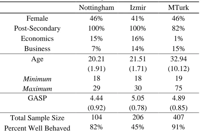
B. Subject Pool Statistics
Table SM.1.1 includes subject pool details for subjects included in the analysis;
that is, subjects who had well behaved preferences (as defined in the main text; see also
below). The first row gives the proportion of female subjects. Post-Secondary refers to
any higher education experience. By default all subjects in the Nottingham and Izmir
subject pools meet this requirement while 82% of the MTurk subjects have had some
amount of post-secondary education. It has been observed that studying economics or
4 analysis. The mean and standard deviation of age is given as well as the minimum and
[image:29.595.137.463.149.363.2]maximum values.
Table SM.1.1. Subject Pool Details.
Nottingham Izmir MTurk
Female 46% 41% 46%
Post-Secondary 100% 100% 82%
Economics 15% 16% 1%
Business 7% 14% 15%
Age 20.21 21.51 32.94
(1.91) (1.71) (10.12)
Minimum 18 18 19
Maximum 29 30 75
GASP 4.44 5.05 4.89
(0.92) (0.78) (0.85) Total Sample Size 104 206 407 Percent Well Behaved 82% 45% 91%
In the first three sections of the table, subject pool details are given only for subjects whose revealed preferences were well behaved. GASP denotes the score from the
guilt and shame proneness scale by Cohen, et al. (2011). A GASP score = 1 (7) indicates low (high) levels of guilt and shame proneness. The fourth section includes
information about all participants.
C. Order of Tasks
The order of tasks in our experimental sessions was the Blanco et al. (2011) Modified
Dictator game and Ultimatum game plus two public goods games (greater details given
below) followed by the scenario tasks. This order was chosen to preclude spillover effects
from the scenario tasks into the games. We assumed that spill-overs from games to scenarios
are less likely than from scenarios to games, but, admittedly, we have not tested this
assumption. Each participant made decisions in all the roles of each game using the strategy
method where necessary. A game was randomly selected for payment at the end of the
experiment (the selection of each game had equal chance, as did each assignment of roles).
5 we measured earnings in points which were exchanged into local currency at the end of each
session.1
The public goods games are not analyzed in this paper, but, for sake of completeness, we
report what we did. Subjects participated in two two-player one-shot public good games
following the same procedures as Fischbacher et al. (Journal of Economic Psychology 33(4),
897-913, 2012). In the first public good game – known as the P-experiment in Fischbacher et
al. (2012) – subjects’ contribution preferences were elicited using a form of the strategy
method. In the second public good game – known as the one-shot C-experiment – subjects’
report their belief about their co-player’s contribution and then their own contribution.
Subjects did not receive any feedback until after completing the scenario task. The
feedback they received was twofold: (1) after all the games and scenario tasks were
completed but before the questionnaire subjects learned which of the four games would be
payoff relevant (in the Nottingham and Izmir experiments; in the MTurk experiment they
received this information after completion of the MTurk HIT) and (2) only after completion
of the questionnaire did participants see feedback and at this time they received feedback
only on the payoff relevant game (again for the MTurk subjects, they received this
information after the completion of the MTurk HIT).
D. Assigning Revealed Preferences Values
We also follow Blanco, et al. in assigning βi=1 (resp. βi=0 ) to subjects who always (resp.
never) choose the equal distribution; and in excluding subjects with multiple switch points in
the Modified Dictator Game from the analysis. We likewise follow Blanco et al. and assign
1 In the UK, 1 point = 0.75 pence; in Turkey, 1 point = 1.5 Turkish Lira; and on Amazon Mechanical Turk, 1
point = 17.5 cents. Exchange rates were chosen to equalize purchasing power as much as possible in the student
subject pools. Since MTurk is a naturally occurring work-place, a different payment structure (with a higher
6 participants who do not reject any offers an αi=0 and participants who reject every offer
below the equal split, an αi=4.5 (although in theory these participants could have αi≥4.5).
Subjects with multiple switch points in the Ultimatum Game are excluded from the analysis
in both the main paper and supplementary materials. In summary, subjects were excluded
from the analysis by having:
Multiple switch points in the Modified Dictator Game alone
Multiple switch points in the Ultimatum Game alone
7
II.
Section SM.2. Full Instructions of the Experiment
A. Background
Included here are the full instructions for the Nottingham subject pool. These
instructions were based off of those by Loewenstein et al. (1989) for the scenarios and
Blanco et al. (2011) for the Modified Dictator game and Ultimatum game. Blanco et al.
(2011) kindly provided instructions and copies of the zTree files which were used in this
experiment with only minor modifications. The text and all the materials including the
zTree files for the Izmir subject pool were translated (both forward and reverse) into
Turkish. In both Nottingham and Izmir, the experiments were conducted by native
speakers and supervised by one of the authors [Beranek]. The Turkish version of
scenarios and instructions, as well as all zTree files are available upon request.
The MTurk participants completed the experiment online using the online survey
software Qualtrics via MTurk and the text and materials were Americanized. These
materials are available upon request in the form of a PDF file.
B. Instructions
Economic Research Project
You are now taking part in an experiment. If you read the following instructions carefully,
you can, depending on your and other participants’ decisions, earn a considerable amount of
money. It is therefore important that you take your time to understand the instructions. Please
do not communicate with the other participants during the experiment. Should you have any
questions, please ask us.
The experiment consists of four different sections. In each section you will be called to make
one or more decisions. You will have to make your decisions without knowing other
participants’ decisions in the previous sections. Note further that the other participants will
8 Only one of the sections will be taken into account in determining your final payoff. This will
be randomly determined as described below. Each section has the same probability of being
selected. You should take your time to make your decision. All the information you provide
will be treated anonymously.
The section that will be taken into account in determining your final payment will be
selected as follows. Participant Number 2 was randomly chosen at the very beginning of
the experiment. This participant will draw a ball from a cloth bag after all participants have
completed all sections. Each ball in the cloth bag has a different colour and each colour
corresponds to a different section: yellow, blue, green, and red. The resulting colour and
corresponding section will be used to calculate your payment.
The computer will randomly pair you with another participant in the room and will assign the
roles. The matching and roles assignment will remain anonymous. You will not know which
role you were playing until the end of the game.
Your earnings will be paid to you in cash at the end of the experiment at a rate of 1 point = 50
pence. Earnings will be confidential.
Yellow Section
In this section the situation is as follows:
Person A is asked to choose between two possible distributions of money between her
and Person B in twenty-one different decision problems. Person B knows that A has
been called to make those decisions, and there is nothing he can do but accept them.
The roles of Person A and Person B will be randomly determined at the end and will
remain anonymous
Before making your decisions please read carefully the following paragraphs.
The decision problems will be presented in a chart. Each decision problem will look like the
following:
Person A's Payoff Person B's Payoff Decision Person A's Payoff Person B's Payoff
9 You will have to decide as Person A; hence if in this particular decision problem you choose
left, you decide to keep the 20 points for yourself so Person B’s payoff will be 0 points.
Similarly, if you choose Right, you and the Person B will earn 5 points each.
You will need to choose one distribution (Left or Right) in each of the twenty-one rows you
will have in the screen. If this is chosen as the payoff relevant section, the computer will
randomly choose one of the twenty-one decisions. The outcome in the chosen decision will
then determine your earnings.
The computer will randomly pair you with another participant in the room and will assign the
roles. The matching and roles assignment will remain anonymous.
Please note that you will make all decisions as Person A but the computer might assign you
Person B’s role.
If you are assigned the role of A, you will earn the amount that you have chosen for Person A
in the relevant situation and the person paired with you will earn the amount that you have
chosen for Person B.
In the case that you are assigned the role of Person B, you will earn the amount that Person A
whom you are paired with has chosen for Person B in the relevant situation.
Blue Section
In this section the situations is as follows:
Person A is asked to choose one out of twenty-one possible distributions of money
between her and Person B. Person B knows that A has been called to make these
decision, and may either accept the distribution chosen by A, or reject it.
In the case that Person B accepts A’s proposed distribution, that will be implemented.
If B rejects the offer, both receive nothing.
The roles of Person A and Person B will be randomly determined by the computer
and will remain anonymous.
Before making your decision please read carefully the following paragraphs.
In the case that this section is selected to determine your earnings, the computer will
randomly pair you with another participant in the room and will assign the roles. The
10 You will have to make decisions as if you were Person A and also as if you were Person B. In
the latter case, you will have to decide whether you accept or reject each of A’s possible
twenty-one proposed distributions.
If you are assigned the role of Person A you will earn the payoff you chose for yourself if the
Person B that you are paired with accepts your offer. Otherwise, you both will earn nothing.
If you are assigned the role of Person B, you will earn the payoff that the Person A that you
are paired with chose for B, only if you had accepted that particular offer. Otherwise, you
both earn nothing.
Green and Red Sections
[These sections were unrelated to this paper.]
Scenarios and Questionnaire
Scenarios
In this section of the project you will read two different scenarios. After reading each
scenario, you will learn the outcome of the situation with a variety of payoffs for you and
another party. Your task in this section is to rank your satisfaction with the various payoffs to
yourself and the other party on a scale from very unsatisfied (-5) to very satisfied (5). Keep
in mind that the order of the payoffs is randomly displayed, so you should be certain to rank
your satisfaction of each outcome according to its corresponding payoffs listed to the left of
the radio button input scale.
Questionnaire
While calculating your payoff, we would like to ask you to answer the following
questionnaire.
Please answer each of the following questions as accurately as possible. Of course, your
answers will be treated confidentially. Your honest answers will be of immense value for our
11
III.
Section SM.3. Determining Stated Preferences of Inequality
Aversion.
A. Design of the Loewenstein et al. Experiment
The scenario tasks provide a near replication of the Loewenstein et al. (1989) (henceforth
“LBT89”) Study Two scenario tasks with a few exceptions noted below. Participants are
asked to rate their satisfaction for outcomes to two scenario disputes. Not every participant
faces the same scenarios; dispute type and relationship condition vary across the treatments.
The disputes are regarding the gains or losses from disputes involving an invention and from
the mutual ownership of a plot of land.
In the original LTB89 paper, the invention scenario regarded the development of
cross-country water skis. We developed an alternative invention scenario regarding the
development of a smartphone application which is identical in structure to the 1989 scenario,
but we expect to be more readily comprehensible to our subjects.
The relationship condition is either a positive or a negative condition and is elaborated in
the scenario descriptions. In the MTurk sample, we also included a third condition where
there was no relationship manipulation; that is, the nature of the relationship was not
mentioned. We refer to this condition as neutral.
We made small adaptations to the scenario text to reflect the individual characteristics of
the subject pools – we have an Anglicized version for the Nottingham subject pool, an
Americanized version for the MTurk subject pool, and a Turkish version for the Izmir subject
pool. The text and all the materials of the Izmir subject pool were translated (both forward
and reverse) into Turkish. In both Nottingham and Izmir, the experiments were conducted by
native speakers. The scenario text for the Nottingham subject pool is included below.
12 This was a 2x2x2 design and participants were randomly assigned to each dispute and
relationship condition in such a way that they rated both gain and loss conditions for either
(a) the invention dispute with a positive relationship condition and the plot dispute with a
negative relationship condition or (b) the invention dispute with a negative relationship
condition and the plot dispute with a positive relationship condition. For each of the four
scenarios, the task is to rate 21 distributions of payoffs for the subject and another person
described in the scenario. Each subject is presented with four (out of the eight) scenarios and
therefore asked for a total of 84 ratings on a scale from -5 representing “very unsatisfied” to 5
representing “very satisfied.”
The gain conditions are classified as 300, 500, and 600 received to self while the positive
outcomes to the other player range from 0 to 900. The loss conditions are the same unit
amounts expressed as amounts to pay and not profit. Following the procedures outlined by
LTB89, the outcome pairs are randomly ordered to avoid automatic responding. The zTree
screen shots from the invention dispute as presented to the Nottingham subject pool are
included below in Figure SM.3.1.
We also included a neutral relationship condition in the American MTurk sample to see
what extent the relationship frame impacted utility ratings. In those cases, no relationship
information was given to the participants. In this case, this was a 2x3x2 design and
participants were randomly assigned to dispute and relationship conditions.
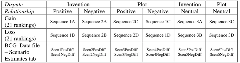
Table SM3.1 summaries the sequences detailing the dispute and relationship conditions
present in each as well as referencing the output from the OLS estimations which are
13 Table SM.3.1. Summary Scenario Sequences and Resulting OLS Estimates
Dispute Invention Plot Invention Plot
Relationship Positive Negative Positive Negative Neutral Neutral
Gain
(21 rankings) Sequence 1A Sequence 2A Sequence 2C Sequence 1C Sequence 3A Sequence 3C
Loss
(21 rankings) Sequence 1B Sequence 2B Sequence 2D Sequence 1D Sequence 3B Sequence 3D
BCG_Data file – Scenario Estimates tab Scen1PosDiff Scen1NegDiff Scen2PosDiff Scen2NegDiff Scen3PosDiff Scen3NegDiff Scen4PosDiff Scen4NegDiff Scen5PosDiff Scen5NegDiff Scen6PosDiff Scen6NegDiff
Subjects participated in one of three sequences. In each, they first read the Invention Dispute
and then ranked their satisfaction with 21 gain distributions (either Sequence 1A, 2A, or 3A) and then 21 loss distributions (either Sequence 1B, 2B, or 3B).
Next, they read the Plot Dispute and then ranked their satisfaction with 21 gain distributions
(either Sequence 1C, 2C, or 3C) and then 21 loss distributions (either Sequence 1D, 2D, or 3D).
The sequences varied according to relationship condition: Sequence 1 had a positive
relationship frame for the invention dispute and a negative relationship frame for the plot
dispute; Sequence 2 had a negative relationship frame for the invention dispute and a positive relationship frame for the plot dispute; and Sequence 3 had neutral relationship frames for both (only half the MTurk participants participated in sequence 3).
We used each of these rankings as the dependent variable in an OLS estimation for the
functional form below with the independent variables being own payoff and the difference between own and other payoff. Each of the sequences resulted in four different OLS
parameter estimates (two for NegDiff and two for PosDiff) that can be found in the Scenario
Estimates tab of the BCG_Data file which is available as a supplementary file in Excel
format.
The two NegDiff (PosDiff) estimates are averaged together between the scenarios in order
to create the Stated a (Stated b)variables (see discussion in section SM.3.C – particularly page 26 – for further explanation and Table SM.3.2 for evidence supporting this procedure).
B. Scenario Texts
The scenarios were structured in the following way: first, the dispute is introduced;
second, a relationship condition is introduced – positive or negative (or neutral in the MTurk
subject pool); third, subjects rank their satisfactions with 21 gain distributions and 21 loss
distributions. Participants do this entire sequence with two different scenarios for a total of 84
14
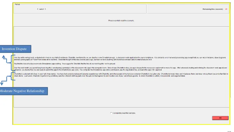
1. Smartphone App Scenario (Updated 2012 version of the 1989 Patent Scenario)
with Moderate Relationships, Anglicized
a. Dispute: “One day while eating lunch, a student who lives in your
residence hall, Charlotte, mentioned to you an idea for a new Smartphone
app: a classroom note application for your smartphone. It is similar to a
normal word processing app except that you can record lectures, draw
diagrams, and take photographs of PowerPoint slides all in real time.
Charlotte thought of the idea several years ago, but had not done anything
with it and had not been able to interest anyone in it. You find the idea of
a classroom note Smartphone app exciting. You suggest to Charlotte that
the two of you work together on the project. Over the next month you
spend long hours together constructing a prototype of the classroom note
app in the computer room. Since it was Charlotte’s idea, you agree to pay
the rent for the computer room space while you make the app. After
extensively testing and refining the classroom note app at your university,
you decide that you are ready to submit the app to the Smartphone app
store. You complete the Smartphone app store submission, pay the
registration fee, and send the app in for approval.”
b. Relationship:
i. Moderate positive relationship: “Charlotte is a student in your
residence hall. You like Charlotte a lot, and other people in the
dorm also consider Charlotte to be very nice. Charlotte takes notes
and picks up assignments for people who miss classes. Last week,