An optimally efficient technique for the solution of systems of nonlinear parabolic partial differential equations

An Optimally Efficient Technique for the

Solution of Systems of Nonlinear Parabolic

Partial Differential Equations

F.W. Yang

, C.E. Goodyer

, M.E. Hubbard

and P.K. Jimack

1_{Department of Mathematics, University of Sussex, Brighton, United Kingdom} 2_{ARM, York House, Manchester, United Kingdom}

3_{School of Mathematical Sciences, University of Nottingham, United Kingdom} 4_{School of Computing, University of Leeds, United Kingdom}

June 5, 2016

Abstract

This paper describes a new software tool that has been developed for the efficient solution of systems of linear and nonlinear partial differential equations (PDEs) of parabolic type. Specifically, the software is designed to provide optimal compu-tational performance for multiscale problems, which require highly stable, implicit, time-stepping schemes combined with a parallel implementation of adaptivity in both space and time. By combining these implicit, adaptive discretizations with an opti-mally efficient nonlinear multigrid solver it is possible to obtain computational solu-tions to a very high resolution with relatively modest computational resources. The first half of the paper describes the numerical methods that lie behind the software, along with details of their implementation, whilst the second half of the paper illus-trates the flexibility and robustness of the tool by applying it to two very different example problems. These represent models of a thin film flow of a spreading vis-cous droplet and a multi-phase-field model of tumour growth. We conclude with a discussion of the challenges of obtaining highly scalable parallel performance for a software tool that combines both local mesh adaptivity, requiring efficient dynamic load-balancing, and a multigrid solver, requiring careful implementation of coarse grid operations and inter-grid transfer operations in parallel.

Keywords: parallel, adaptive mesh refinement, finite difference, implicit, multigrid, thin film flow, tumour growth.

1

Introduction

Many problems in computational engineering and science are based upon the use of complex mathematical models and their numerical approximations. These models of-ten consist of highly nonlinear, time-dependent and coupled PDEs. Accurate, efficient and reliable numerical algorithms (and, frequently, great computational power) are necessary in order to obtain robust computational solutions. This paper describes a new Engineering Software tool that we have developed to exploit advanced numeri-cal methods for the efficient solution of nonlinear time-dependent systems of PDEs. Specifically, the focus of this software is nonlinear, and potentially stiff, parabolic systems. This type of system may be used to represent a plethora of different ap-plications, ranging from solidification [4] and computational fluid dynamics [2, 5] to tumour growth [3].

The multigrid method is commonly accepted as being one of the fastest numerical methods for solving algebraic equations arising from mesh-based discretizations of PDEs. Brandt in his 1977 paper [6] systematically describes the first multigrid meth-ods, and some of their applications. Subsequent publications, e.g. [15, 8], suggest further combinations of multigrid methods with spatial adaptivity and adaptive time-stepping, for applications in which physical effects occur at multiple length and time scales. In recent years a number of general-purpose software packages have been de-veloped to provide adaptive multigrid solvers for broad classes of PDEs. Noteworthy examples include DEAL.II [9] and DUNE [10]. The software that we introduce in this paper is intended to complement such general-purpose packages by providing a tool that we have developed specifically for the solution of multiscale parabolic PDE systems using fully-implicit time stepping. Typically these problems are highly stiff, thus requiring strongly stable temporal discretization, which leads to large systems of (generally nonlinear) algebraic equations to be solved at each time step. Our solver is written specifically with such systems in mind, and exploits nonlinear geometric multigrid methods in order to advance in time with optimal efficiency.

The particular nonlinear multigrid scheme that we use is based upon a combina-tion of the multilevel adaptive technique (MLAT) and the full approximacombina-tion scheme (FAS), first introduced in [15] and [6] respectively. These are implemented in a par-allel setting based upon distributed memory parpar-allelism using the MPI library, and this paper describes our new software framework for the first time. In addition to this overview of the software, we also include a thorough evaluation of our implementation and the effectiveness of our chosen computational techniques. This is acheived using two example applications which are based upon (i) the thin film flow of a spreading droplet [2], for which we demonstrate the temporal and spatial adaptivity in detail; and (ii) a multi-phase-field model of tumour growth, which was also discussed in [11].

2

Software Framework

In this section, we provide an introduction to our software with its key features. This is followed by a high level overview of the programme flow and then enhanced details of the the main components of our software tool. Afterwards, various implementation issues are explained, and the section ends with a description of the user’s control of the software.

2.1

Introduction

The purpose of this paper is to describe a new software tool, Campfire, which we have developed in order to efficiently obtain solutions to general systems of nonlinear parabolic PDEs. The core of the software is the use of nonlinear multigrid methods to solve the algebraic systems arising from implicit temporal discretization schemes. The user is free to select their own spatial discretization scheme based upon cell-centred quadrilateral or hexahedral elements (i.e. the degrees of freedom are stored at the cell centres). Finite difference, low order discontinuous Galerkin and finite volume meth-ods are typical examples that may provide such cell-centred discretizations, though we make use only of the former in all of the examples presented in this paper.

Distinctively, our nonlinear multigrid solver has optimal, linear, computational complexity for general systems of parabolic PDEs (illustrated in Section 3). The software is able to include spatial and temporal adaptivity, and parallel computing is implemented through geometric domain decomposition. This combination of tech-niques gives a huge boost to the efficiency, thus allowing complex, time-dependent systems to be solved in 3-D within reasonable and practical time.

Campfire is designed to be flexible and efficient. It only requires the user to sup-ply the fully-discretized system (in the form of a residual function), the initial and boundary conditions of the model and prescribed parameter values. Most of the func-tionalities within this software can be easily adjusted by altering these parameters, though robust default values for general cases are also provided.

For clarity, we summarise the key features of our software:

• it is able to carry out the computation in a parallel environment where the par-allelization comes from mesh partitions via domain decomposition;

• it is able to generate a distributed mesh hierarchy using an open source library (i.e. PARAMESH [1]), with appropriately modified mesh data structures and dynamic load-balancing procedures, tuned for enhanced parallel multigrid per-formance;

• it is able to dynamically adapt the spatial mesh in a hierarchical manner based upon flexible error control criteria;

upon numerical stability constraints);

• it is able to solve the nonlinear algebraic systems arising from the adaptive spa-tial and temporal discretizations using nonlinear multigrid methods, [6, 15];

• it is able to store checkpoint files for possible restarts in parallel environments via HDF5;

• it is able to output solutions into standard formats (e.g. CSV and VTK) for common visualization tools such as Paraview [12].

This paper is the first description of the software tool itself, however, earlier versions of the multigrid solver, that are now part of the software, have been used in [4, 13] to solve specified problems in the solidification of metallic alloys.

2.2

Overview

In Campfire the user is able to define their own spatial discretization based upon cell-centre values in the hexahedral mesh (in the 3-D case). Combining this with an im-plicit temporal discretization leads to a system of algebraic equations for which there are unknown values at the centre of each hexahedron (one unknown for each depen-dent variable) at the end of each time step. Throughout this section we represent this system of equations as either

F(u) = 0 or A(u) = f . (1)

Hereustores all of the unknown values to be determined at the end of the time step, whilstF andAare nonlinear functions related byF(u) =A(u)−f for some known vectorf.

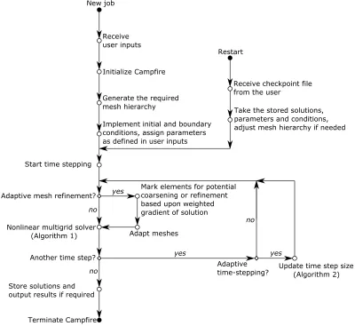
In order to commence a new simulation in Campfire it is necessary to provide a set of parameters that define the problem and control the mesh adaptivity (see sub-section 2.4.2), and a set of initial conditions for each dependent variable (see subsec-tion 2.4.1). These are used to initialise the software (including memory allocasubsec-tion), to allocate an initial spatial mesh (with the support of the PARAMESH library) and to assign the initial state of the necessary variables (see subsection 2.4.1). This initializa-tion process is indicated by the “New job” branch in Figure 1. Further details of the mesh data structure and the key parameters, as well as how to define the discrete PDE system, are provided in the next section: the purpose of Figure 1 is to describe how Campfire operates at a high level, and how the key components are linked together. Note that it is also possible to re-start a previous run from a checkpoint file, as indi-cated by the “Restart” branch in the same figure. The HDF5 checkpoint file allows all previous mesh and solver parameters to be picked up and the previous run to be continued from that point in time onwards.

New job

Receive user inputs

Implement initial and boundary conditions, assign parameters as defined in user inputs Generate the required mesh hierarchy

Start time stepping

Restart

Receive checkpoint file from the user

Take the stored solutions, parameters and conditions, adjust mesh hierarchy if needed

Adaptive mesh refinement?

Mark elements for potential coarsening or refinement based upon weighted gradient of solution Adapt meshes Nonlinear multigrid solver

(Algorithm 1) Another time step?

Adaptive

time-stepping? Update time step size _{(Algorithm 2)} Store solutions and

output results if required

Terminate Campfire

Initialize Campfire

no no

yes

yes

no

yes

(AMR) based upon the latest solution values; the use of the nonlinear multigrid solver for the nonlinear algebraic system of equations, of the form (1), that arises at the current time step; and the selection of the step size for the next time step (adaptive time-stepping). We now describe these three components in further detail.

The AMR algorithm is fairly standard and is described in full in [1]. As explained in Section 2.3.1, it is based upon hierarchical refinement through the use of a quad-tree or an oct-tree (in two or three dimensions respectively) data structure. Each node of the tree is a block of uniform mesh (e.g. 16×16×16hexahedral elements) which may be refined into four or eight child blocks (in two or three dimensions). The al-gorithm is divided into two phases: the first decides which blocks should be refined or coarsened (based upon either a default error indicator or a user-supplied error in-dicator, along with some constraints on the mesh topology (e.g. neighbouring blocks cannot differ by more than one level of refinement)); whilst the second phase actually implements the refinement. For this second phase, not only is the tree data structure updated to reflect blocks which are refined or coarsened (for coarsening, it is effec-tively the inverse of a refinement operation so, in three dimensions, eight child blocks would be removed from the tree and the memory freed), but a dynamic load-balancing routine is then invoked so as to ensure that the mesh tree is equally partitioned across the available processes. In the default version of PARAMESH the tree is partitioned based upon the partition of a depth-first ordering (referred to as Morton ordering), however this is very unsuitable for multigrid solvers since the finest mesh level (where most computational work takes place (see below)) will not generally be split equally amongst the processes. Hence we use a dynamic load-balancing strategy which parti-tions all of the blocks that lie at the same depth of the tree independently: each of these partitions aims to provide an equal number of blocks per process, and neighbouring blocks allocated to the same process where possible (so as to minimize inter-process communication).

below a prescribed absolute value or a prescribed relative reduction from the initial residual, convergence is assumed (and if neither criterion is met after a maximum number of iterations the time step is repeated with a smaller step size). Further details of the smoother, the grid transfer operators (I2h

h and I2hh) and the default parameters

used for each V-cycle are given in the following sections.

Algorithm 1V-cycle MLAT nonlinear FAS multigrid method

The superscriptshand2hdenote fine and coarse grid (Ωh andΩ2h) values

respec-tively.

Function:Function:Function:uh_{= V-cycleMLATMG(h, u}h_{, u}2h_{, f}h_{, f}2h_{, A}h_(uh_{), A}2h_(u2h₎₎ 111...Applyp1iterations of the pre-smoother onAh_(uh_{) =f}h

uh _{=PRE-SMOOTH(p1, u}h_{, A}h_(uh_{), f}h₎ 2.

2.

2.Compute the residualrh_onΩ h rh _=fh_−Ah_(uh₎

3.

3.

3.Restrict the residualrh_fromΩ

h toΩ2h∩Ωh to obtainr2h r2h _=I2h

h rh 4.

4.

4.Restrict the fine grid approximate solutionuh _fromΩ

htoΩ2hto obtainw2h

w2h ₌

(

I2h

h u

h _onΩ

2h∩Ωh

u2h _{on the remaining part ofΩ} 2h 5.

5.

5.Compute the modified RHS

f2h ₌

(

r2h _+A2h_(w2h_{) onΩ}

2h∩Ωh

f2h _{on the remaining part ofΩ}

2h 6.

6.

6.ifififΩ2h =coarsest grid thenthenthen

Perform an “exact” coarsest grid solve onA2h_(u2h_{) = f}2h

elseelseelse

u2h _{= V-cycleMLATMG(2h, w}2h_{, u}4h_{, f}2h_{, f}4h_{, A}2h_(u2h_{), A}4h_(u4h₎₎

end ifend ifend if

7.

7.

7.Compute the error approximatione2h _onΩ

2h∩Ωh e2h _=u2h_−w2h

8.

8.

8.Update solution on the remaining part ofΩ2h u2h _=u2h latest

999...Interpolate the error approximatione2h_fromΩ

2htoΩh to obtaineh

eh _=Ih

2he2h 101010...Perform correction

uh _=uh_+eh

111111...Applyp2 iterations of the post-smoother onAh(uh) =fh uh _{=POST-SMOOTH(p2, u}h_{, A}h_(uh_{), f}h₎

Finally, we describe the adaptive time-stepping procedure. There are two main options for controlling the adaptive time-step selection in Campfire: either selecting

former in Algorithm 2 since this is the default setting in Campfire, and is independent of the time-stepping scheme being used. As may be seen from Algorithm 2, when a converged solution is obtained at the previous time step in a low number of multigrid V-cycles the time step size will be increased (subject to a maximum value which can be set by the user). Otherwise, if convergence is not achieved at the previous time step in a prescribed maximum number of V-cycles then the step size is reduced by 25%

and the previous step is retaken. Alternatively, if convergence was achieved at the previous time step, but at a slower rate than targeted (i.e. a high number of V-cycles were taken), then the step size is reduced by 10% for the next time step. After the algebraic system is solved or the maximum number of V-cycles is reached (i.e. slow convergence or non-convergence respectively), the number of V-cycles and the norm of the residual can be assessed. If none of the above occurred then convergence was neither too slow nor excessively fast and soδtis left unchanged for the next step. All of the parameter values for measurements in the if-statements, as well as the different ratios of changes toδt, may be altered by the user. Note we use the superscriptsτ+ 1

andτ to indicate the next time step size and the current step size, respectively.

Algorithm 2Adaptive time stepping in Campfire

1.

1.

1.Input: No.V-cycles – the number of V-cycles that are used by the multigrid solver at this time step

2.

2.

2.Input : r– residual

3.

3.

3.ififif No.V-cycles is low andandandris acceptable thenthenthen

4.

4.

4. δtτ+1 ₌ 10 9δt

τ

555... ifififδtτ+1 _{≥max-δt-allowed thenthenthen}

666... δtτ+1 _{=max-δt-allowed}

777... end ifend ifend if

888...else ifelse ifelse if No.V-cycles reaches the maximum number orororris not acceptable thenthenthen

999... Recompute the current time stepτ withδtτ ₌ 3 4δt

τ

10.

10.

10.else ifelse ifelse if No.V-cycles is high thenthenthen

11.

11.

11. δtτ+1 ₌ 9 10δt

τ

121212...end ifend ifend if

The above descriptions summarise the general computational flow within Campfire as well as its essential components. In the next section, we provide details of some of the key implementation issues.

2.3

Key Algorithmic Details

2.3.1 Parallel Adaptive Mesh Refinement

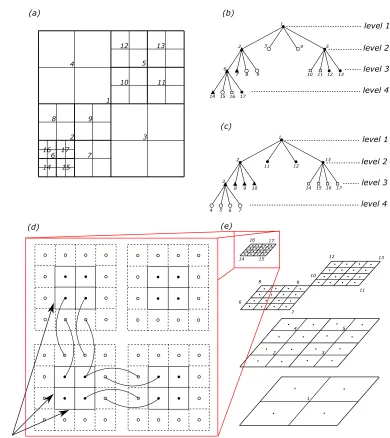
One of the fundamental building blocks in Campfire is its mesh structure, which is inherited from the open source software library PARAMESH [1]. This structure is based upon a dynamic tree of Cartesian mesh blocks of a fixed size (a quad-tree in 2-D or an oct-tree in 3-D). To illustrate, we use an simple 2-D adaptive grid with a coarse block size as an example. This example is shown in Figure 2 (a), with a user-defined block size of2×2(note this size choice is for the purpose of demonstration: in practice, sizes like 8×8or 16×16(or 16×16×16in 3-D) are usually used). As shown in this figure, despite different refinement levels, all mesh blocks have this selected size of 2×2. We include a "telescope" view of the example adaptive grid in Figure 2 (e) where we use solid dots to represent the cell-centred grid points. In (a) and (e), the heavy lines indicate the boundaries of each block, and the lighter lines indicate individual cells.

Parallelism is achieved through distributing mesh blocks to multiple MPI pro-cesses, and using MPI to communicate between individual MPI processes to exchange data. An important concept is that of guard cells. Each mesh block is surrounded by a layer of guard cells, which may be expanded to multiple layers for schemes with larger stencils. We illustrate this concept using the four mesh blocks on the finest level of our example. This is shown in Figure 2 (d), where the guard cells are marked using dashed lines and the guard cell centres are indicated by ◦. The guard cells at the actual domain boundary contain information which allows the specified boundary conditions to be implemented, and others are used to store values of corresponding grid points on the neighbouring blocks (the linked curves show the corresponding grid points between neighbours). Thus the parallel communication is used to update the data held by these guard cells.

The quad-tree structure corresponding to the mesh illustrated in (a) and (e) is shown in Figure 2 (b). We use four shapes (i.e. N_{,◦,and•) to indicate a possible partition}

across four MPI processes in a parallel environment. Note this is not the original, so-called Morton ordering used in PARAMESH, but the modified version from Campfire. For completeness, the Morton ordering (if applied to this example) is shown in Figure 2 (c). From a multigrid point of view, the parallel distribution in (a) is superior since the work is partitioned equally at each level, most importantly the finest level.

2.3.2 Nonlinear Multigrid

There are two key components to the nonlinear multigrid solver described in the pre-vious section: steps1and11of Algorithm 1 require an iterative smoother, whilst data transfer operators are needed to perform the restriction and the interpolation in steps

3,4and9.

1

2 3

4 5

6 7 8 9

10 11 12 13

14 15 16 17

(a) (b)

1

2 3 4 5 6

7 8 9 10 11 12 13 14 15 16 17

(c)

1 2

3

4 5 6 7 8 9 10

11 12 13

14 15 16 17

level 1

level 2

level 3

level 4

level 1

level 2

level 3

level 4

(d)

1 2 3

4 5 6

7 8

10

11 12 13 14 15

16 17

9

(e)

boundary

Let us consider a cell-centred finite difference discretization at each implicit time step: F(u) = 0, whereuis a vector containing all unknown values at the end of the step. Let ui,k be the approximate solution on grid point i for unknown variablek,

where we assumeKunknowns at each grid point. The systemF(u) = 0is made up ofN × Kcoupled nonlinear algebraic equations (whereN is the number of internal, cell-centred grid points), each of the form

Fi,k(u) = 0, (2)

wherei = 1, . . . , N andk = 1, . . . ,K. To clarify the notationui,kis thekth

compo-nent ofui ∈RKandFi,kis thekthcomponent ofFi ∈RK. On one grid pointi, allK

variables may be updated simultaneously as

uℓi+1 =uℓi −C

−1

i Fi(uℓ), (3)

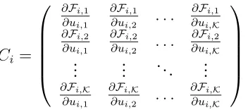
whereℓis the iteration index andCi−1is the inverse of theK×Klocal Jacobian matrix Ci, which is given as

Ci =

     

∂F_i,1 ∂ui,1

∂F_i,1 ∂ui,2 . . .

∂F_i,1 ∂ui,K ∂F_i,2

∂ui,1

∂F_i,2 ∂ui,2 . . .

∂F_i,2 ∂ui,K

..

. ... . .. ...

∂F_i,K ∂ui,1

∂F_i,K ∂ui,2 . . .

∂F_i,K ∂ui,K

      . (4)

This iterative method is also used as the iterative solver on the coarsest grid (i.e. at step 6 of Algorithm 1), by sweeping through the grid multiple times.

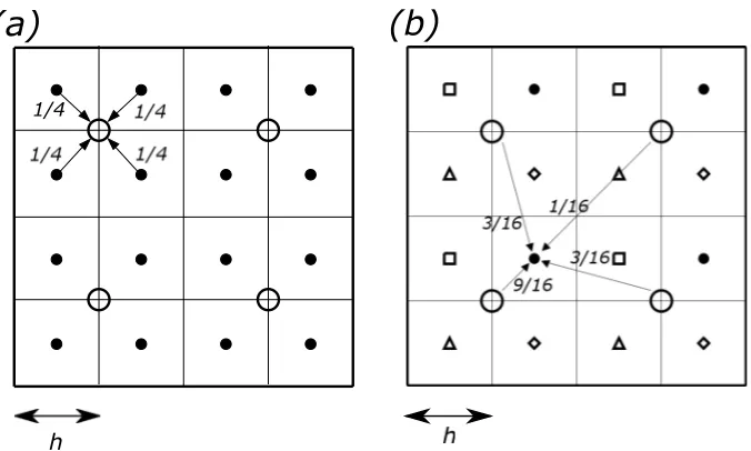
The other key multigrid component introduced in the previous section is the grid transfer operators, used to move data between grid levels. Considering we are us-ing cell-centred grids, a cell-averagus-ing restriction and a bilinear interpolation are em-ployed [8]. We illustrate these two operators on a simple 2-D cell-centred grid in Figure 3. A 2-D version of the restriction can be written as

Ih2huh(x, y) =

1 4

"

uh

x− h

2, y −

h

2

+uh

x− h

2, y+

h

2

uh

x+h

2, y−

h

2

+uh

x+h

2, y+

h

2

#

,

(a)

(b)

h 1/4

Figure 3: (a) The cell-averaging restriction operator in Equation (5): arrows indicate an example of this process from points (marked as•) on the fine mesh level to a point (marked as ◦) on the coarse mesh level. (b) The bilinear interpolation operator in Equation (6): arrows indicate an example of this process from points (marked as◦) on the coarse mesh level to a point (marked as•) on the fine mesh level.

and a 2-D version of the interpolation is given as

Ih

2hu2h(x, y) =

                                       1 16 h

9u2h x− h₂, y−h₂

+ 3u2h x−h₂, y+3₂h

+3u2h x+3₂h, y−h₂

+u2h x+3₂h, y+3₂h

i

for •;

1 16

h

3u2h x− 3₂h, y− h₂

+u2h x− 3₂h, y+3₂h

+9u2h x+h₂, y− h₂

+ 3u2h x+ h₂, y+3₂h

i

for _;

1 16

h

3u2h x− h₂, y−3₂h

+ 9u2h x− h₂, y+h₂

+u2h x+3₂h, y− 3₂h

+ 3u2h x+ 3₂h, y+ h₂

i

for ⋄;

1 16

h

u2h x− 3₂h, y− 3₂h

+ 3u2h x−3₂h, y+h₂

+3u2h x+h₂, y− 3₂h

+ 9u2h x+h₂, y+ h₂

i

for △,

(6)

where the arrayustores values at the grid points,(x, y)are the Cartesian coordinates,

2.4

User Experience

In this section, we provide an overview of how a user of the software can define the problem being solved and control the way in which the solver progresses. As indi-cated above, the key user-defined functions are the residual function, which allows the discretized PDE system to be defined (see Equation (2)), and the local Jacobian ma-trix which contains the derivative terms shown in Equation (4). In the first subsection below we describe the key data structure that must be used in order to define these. In the second subsection, we then provide an overview of the key parameters that may be selected or defined by the user in order to control the model, the domain, the multigrid solver, etc.

2.4.1 User-Defined Functions

Following the approach of PARAMESH [1], within Campfire the key data structure is the so-called “unk” array. This is a multi-dimensional data structure that is synchro-nised to the mesh blocks, making it highly parallelizable. This data structure is also suitable for multiple dependent variables. It is given by

unk(var, i, j, k, lb), (7)

wherevaris described below,i, j, krepresent each grid point (i.e. cell) in the current mesh block andlbdenotes the mesh block. If it is in 2-D,k stays as1.

In Campfire’s default option, there are five arrays associated with each dependent variable. For example, the first variable has the following data structure:

unk(1, i, j, k, lb), stores the latest solution (or the initial condition);

unk(2, i, j, k, lb), stores the modified RHS (or is zero on the finest grid);

unk(3, i, j, k, lb), stores the computed residual value (shown in Equation (2));

unk(4, i, j, k, lb), stores the solution from the previous time step;

unk(5, i, j, k, lb), stores the solution from the one before previous time step.

For a system of PDEs, the second dependent variable then starts with unk(6, i, j, k, lb)

through to unk(10, i, j, k, lb). For example, the thin film model presented in Sec-tion 3.1 has two dependent variables, thus 10“unk” arrays. Furthermore, the tumour growth model presented in Section 3.2 has five dependent variables, hence 25“unk” arrays are employed. It is worth noting that the i, j, k indices also include the guard cells on the current mesh block. Note that unk(5, ., ., ., .)is only used when a multi-step discretization is employed in time, such as the adaptive BDF2 scheme [17].

For each variable, the corresponding3rd _{array of the “unk” arrays is assigned by}

Another user-defined term is the initial condition, which must be assigned to the corresponding1st_{array of the “unk” arrays initially. Later on the data in these arrays}

will be replaced by the most recent solutions for each variable in the system.

The final user-defined subroutine is required to compute the local Jacobian matrix which contains the derivative terms (see Equation (4)). This matrix is stored in an

N ×N array whereN is the number of coupled equations. Each entity specified in Equation (4) must be assigned by the user and, at each grid-point visit in the smoother, this local matrix is re-computed using the corresponding information related to the current grid point.

2.4.2 Software Parameters

In total there are seven categories of user-controlled parameters. In the following paragraphs we provide a high level summary of the key ones, with descriptions and some default values.

1. Mesh setup: first of all, to set up the mesh hierarchy, a mesh block size is to be defined: nxb, nyb and nzb specify the number of cell-centred grid points in each axis direction. It is worth noting there is a trade-off, since a smaller size will create too many guard cells relative to the block size, hence burdening the memory and parallel communication, however a larger size will deteriorate the flexibility of the dynamic load balancing and the adaptive mesh refinement. Referring back to the example used in Figure 2, for clarity, we illustrated using a 2×2 block size. However, by default, Campfire suggests a size of 8× 8

for simulations which would have up to 4 million grid points at the finest level if we were to measure the grid as uniform (i.e. up to2048×2048). For larger simulations, especially in 3-D, we suggest to use16×16in 2-D and16×16×16

in 3-D as the block size.

Related parameters include: nguard which defines the number of layers (de-pends on the choice of discretization stencils) of guard cells and is initially set to be1;maxblocks, which is the maximum mesh blocks allowed for each MPI process;nBx,nByandnBzwhich set the number of mesh blocks on the coarsest level for each axis direction, and generally are set to be 1; lrefine_maxgoverns the maximum number of levels in the mesh hierarchy.

2. Problem setup: we begin with defining the domain size by adjusting grid_min

andgrid_max. For example,grid_min = 0andgrid_max= 1defines a square

domain with size[0,1]×[0,1], or a cube domain with size[0,1]×[0,1]×[0,1]. It is possible to define domains that each axis has a different size. In addition,

total_varsis the number of dependent variables, dt is the initial time step size

andsimulation_timeis the ending timeT.

3. Multigrid setup: p1 and p2 are the number of iterations of the smoother (see

range of 1to 4; solve_count_maxis the maximum number of iterations of the smoother to be carried out as a solver on the coarsest grid;max_v_cycle_count

is the maximum number of V-cycles allowed in each time step (see step 8 in Algorithm 2);mg_min_lvlis the coarsest level for the multigrid solver, in case the root level is not desired. Furthermore, lrefine_max defines the finest grid of the solver, absolute_tol is the absolute tolerance for the stopping criterion

andrelative_tolis the relative tolerance for the stopping criterion. If the infinity

norm of the residual (||r||∞) drops by this amount (comparing against the norm

from the first V-cycle of this time step), or it falls below the absolute tolerance, then we consider the solution to be converged at that time step.

4. Output setup: there are two parameters for output,verbosetakes an integer value between 1 and 4 for the amount of terminal output, where 4 is the most de-tailed output and is for debugging;output_ratedefines the number of time steps between generation of checkpoint files.

5. Model-specific: model-specific parameters can be included in a file to allow all of the model-related components to be grouped together. Tables 1 and 7, in Section 3, show the parameters required by the thin film model and the tumour growth model, respectively.

6. AMR setup: local_adaptation, which takes 0or1as the switch for this function-ality; and ctore and ctode which are the thresholds for mesh refinement and coarsening, respectively.

7. Adaptive time-stepping setup: parameters described here control the adaptive time-stepping, adaptive_TS is the 0 or1 switch (i.e. a fixed time step size is used

when adaptive_TS = 0); low_vcycle_count (see step 3 in Algorithm 2) and

high_vcycle_count (see step 10 in Algorithm 2) are two integer values used

to indicate whether we should increase dt for efficiency or reduce it for accu-racy/stability, based upon the rate of convergence of multigrid at the end of each time step.

Having provided a brief overview of the software that we have developed, in the following section we validate this software by demonstrating its successful application to two very different examples, for which we are able to contrast our results with others published elsewhere, [2, 3].

3

Applications

are taken. Hence, there are some minor notational differences, however we clearly state every variable and notation within each subsection. For example,his generally used as the distance between two adjacent grid points, but in Section 3.1, it means the height of the thin film, and dxis employed instead to represent the distance between grid points in the simulations.

The thin film model, described in Section 3.1, is used to validate the software against existing numerical results, to demonstrate optimal convergence of the non-linear multigrid interation and second order convergence of the numerical results in space and time, and to show the improvements in efficiency obtained by applying adaptivity in space and time. In Section 3.2, a tumour growth model is used to provide further evidence that optimal multigrid convergence and second order convergence of the numerical results are retained when adaptivity mesh refinement is applied, then it is used to highlight parallel performance issues for a larger, three-dimensional, test case. For simplicity, in each of our simulations we consider a domain which, in each coordinate direction, is the same length and divided into the same number of cells (N), sodxis the same in each direction.

Note all the computations were carried out on the HPC service provided at the Uni-versity of Leeds. Each compute node consists of two 8-core Intel E5-2670 2.6GHz processors with 16GB of shared memory per processor (i.e. 2GB per core). The com-putational nodes are connected with “Infiniband” interconnects.

3.1

A Thin Film Flow Model of Droplet Spreading

The physical phenomenon of a liquid droplet spreading on a substrate has been stud-ied in many scientific fields. In each case, a common demand is to obtain a relatively accurate numerical model for which the solution represents a good approximation to real-world experiments [19]. Many such models are suggested in the review paper [20]. The model presented here is very close to the work of Schwartz, Bertozzi and their co-workers in [21, 22, 23, 24], and is derived from the Navier-Stokes equations through the use of the lubrication approximation. The precise model, based upon a precursor film, has been previously described by Gaskell et al. in [2] using a vertex-centred finite difference approximation, and solving the resulting system using the FAS nonlinear multigrid with uniform grids. Here we present solutions that are gen-erated by using our parallel, adaptive multigrid solver in two space dimensions (but representing a 3-dimensional flow of a thin film) and compare them with the results in [2].

Following the lubrication approximation, the resulting non-dimensional model con-sists of two dependent variables: h(x, y, t)and p(x, y, t). The former measures the droplet thickness, and the latter represents the pressure field of the droplet. The Reynolds equation for droplet spreading is given as

∂h

∂t =

∂ ∂x

h3

3

∂p

∂x −

Bo

ǫ sinα

+ ∂

∂y

h3

3

∂p ∂y

h*

Vx(z) g

Moving contact line

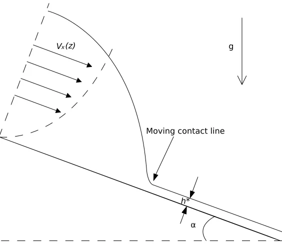
Figure 4: Sketch of precursor film model on an inclined substrate at angleαto the hor-izontal and the parabolic velocityvx(z)in the droplet liquid. Note that h∗ represents

a true thin film ahead of droplet, and the velocity is zero at the substrate.

whereBo is the non-dimensional Bond number, measuring the relative importance of

gravitational force relative to surface tension [22],ǫis the ratio between the character-istic droplet thickness and the extent its footprint on the substrate, and is assumed to be small by the lubrication theory. The main computational challenge is to accurately capture the moving contact line between the thin film liquid and the solid substrate (see Figure 4). Equation (8) is based on the assumption of a no-slip condition at the substrate, however a non-zero velocity is required at the moving contact line (the interface between the air, the drop and the substrate) in order to permit spreading. Figure 4 shows how this “paradox” may be resolved, illustrating a cross-section of the droplet on a substrate inclined at an angleαto the horizontal, as well as a precur-sor film of thicknessh∗

to overcome the no-slip condition at the moving contact line. The physical phenomenon of a thin precursor film has been detected in the real-world experiments presented in [25, 26].

The pressure fieldp(x, y, t)appears in Equation (8) but also needs to be determined. In this model the associated pressure equation is as follows:

p=−△(h+s)−Π(h) +Bo(h+s−z) cosα, (9)

and is given by

Π(h) = (n−1)(m−1)(1−cos Θe)

h∗

(n−m)ǫ2

h∗ h n − h∗ h m , (10)

where n and m are the exponents of interaction potential and Θe is the equilibrium

contact angle. The space derivatives in Equations (8) and (9) are both approximated using standard, second order, centred differences.

The computational domain Ω is chosen to be rectangular with non-dimensional Cartesian coordinates (x, y) ∈ Ω = (0,1)×(0,1). It is further assumed that the droplet is far away from the boundary. Therefore zero Neumann boundary conditions are applied for bothhandp:

∂h

∂ν =

∂p

∂ν = 0 on ∂Ω, (11)

whereνdenotes the outward-pointing normal to the boundary∂Ω.

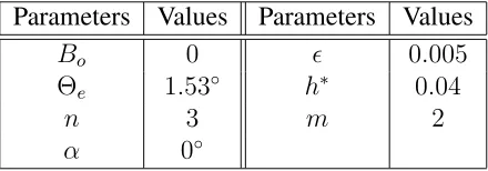
For the purpose of validation, we compare results from using our software to se-lected results presented in [2]. First of all, the values of parameters that are used in the droplet spreading model (Equations (8) to (10)) are presented in Table 1. These values were used by Gaskell et al. in [2].

Parameters Values Parameters Values

Bo 0 ǫ 0.005

Θe 1.53◦ h∗ 0.04

n 3 m 2

α 0◦

Table 1: The parameters of the droplet spreading model that were used by Gaskell et al. in [2].

The initial condition for the variable of droplet thicknessh(x, y, t= 0)is given as

ht=0(r) = max

5

1−320

9 r

2

, h∗

, (12)

wherer2 _=x2_+y2_{. Having obtainedh(x, y, t= 0), the initial condition for pressure} pon all internal grid pointsi, j (i, j = 1, . . . , n) may be defined as

pti,j=0 = 1

dx2

(

hti=0+1,j+h t=0 i−₁,j+h

t=0 i,j+1+h

t=0

i,j−₁−4h

t=0 i,j

)

+ (n−1)(m−1)(1−cos Θe)

h∗_(n−m)ǫ2

h∗ ht=0

i,j

n

−

h∗ ht=0

i,j

m

−Bohti,j=0cosα,

in which it is assumed thats=z= 0.

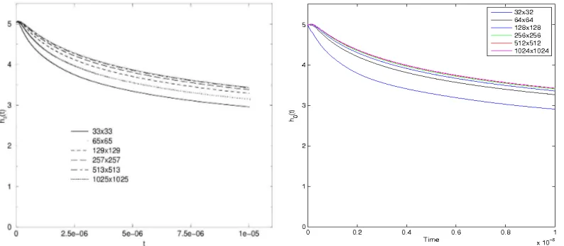
We choose Figure 5(b)from [2] to validate against. This figure shows the evolution of the maximum height of the droplet during simulations. All grids are uniform and the non-dimensional time duration is[0,10−₅

]. In Figure 5, the left-hand side shows a copy of Figure 5(b)from [2]. The right-hand side figure shows the results using our multigrid solver. The maximum height of the droplet is initially5.0, as implied by the initial condition in Equation (12). Figure 5 shows a good agreement with the results from grid hierarchies 1162₋₅₁₂2 _and162₋₁₀₂₄2_{. For the coarser grid hierarchies}

(i.e. 162 ₋₆₄2_{, 16}2₋₁₂₈2 _and162₋₂₅₆2_{), our results appear to be more accurate}

than the ones from [2]. This may be caused by the use of adaptive time stepping in [2], in which the size of the time step is based upon local error estimation, as opposed to our choice of a fixed time step size, systematically reduced in proportion todx on the finest grid.

Figure 5: The evolution of the maximum height of the droplet during simulations, on the left-hand side is Figure5(b)from [2] and on the right-hand side, we show results from our multigrid solver. Parameters used to generate these results are shown in Table 1. Legends in these figures indicate the finest resolutions of grids that are used for each simulation. Note that in the left-hand figure the grid resolution is indicated by numbers of nodes, while in the right-hand figure it is indicated by numbers of cell.

In order to generate these results, we use a 162 _{grid as the coarsest grid (also as}

the block size). There are in total 4smoothing iterations on each grid level, i.e. p1 =

p2 = 2in Algorithm 1, and60iterations of the smoother are used for the coarsest grid solver. The time step size for grid hierarchy162₋₃₂2_{isδt= 3.2×10}−7_{. Each time}

the finest grid is refined, the time step size is halved.

At each time-step, convergence of the multigrid iteration is checked after each V-cycle and the iteration is stopped if either||r||∞ <10−6 or||r||∞/||r₁||∞ < 10−5, in

whichr is the residual (forhorp) andr1 is the residual after the first V-cycle of the current time-step.

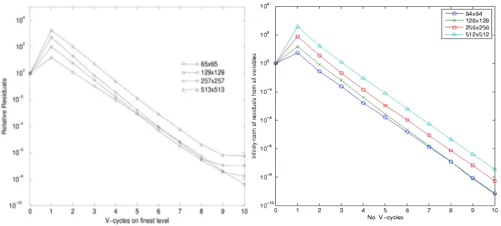
Since the solver from [2] also performs a nonlinear multigrid iteration with FAS, we validate the performance of our multigrid solver against the one used by Gaskell et al. More specifically, we validate the convergence rate of each multigrid V-cycle for a typical time step, based upon the infinity norm of residuals. This is shown in Figure

4(b)from [2]. In Figure 6, the left-hand side shows the performance of the solver used in [2]. On the right-hand side is the performance of our multigrid solver. For both solvers, a total number of10V-cycles within this particular time step are performed. From this figure, the results suggest that both solvers perform similarly. It is worth noting there is one significant difference. In the results from [2], the convergence rate deteriorates significantly from the9th_{V-cycle to the10}th_{V-cycle. However, the results}

from using our multigrid solver remain robust in this situation. This may be due to the use of a different spatial discretization in [2] to the cell-centred scheme used in this work. Overall these tests provide excellent validation.

Figure 6: Convergence rate of a typical multigrid V-cycle for a single time step. On the left-hand side is Figure4(b)from [2] and on the right-hand side are the results of our multigrid solver. Four different finest grid resolutions are used, as shown in the legends. Parameters that are used to generate these results are shown in Table 1.

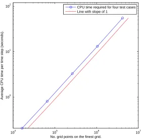
From the right-hand side of Figure 6, we also see that all the curves are nearly parallel, which implies the reduction in the residual is independent from the sizes of the grids. This optimal convergence rate is the goal of multigrid methods, and indicates that the complexity of our multigrid solver is linear. We summarise the CPU time costs from five simulations in Figure 7, with finest grid sizes of1282_,2562_,5122_,

10242 _{and 2048}2_{, respectively. As we quadruple the number of points on the finest}

grid, we also halve the time-step size, and all simulations finish at the same end time

T = 1× 10−₅

104 105 106 107 100

101 102

No. grid points on the finest grid.

Average CPU time per time step (seconds).

CPU time required for four test cases Line with slope of 1

Figure 7: A log-log plot of the CPU time per time step against the total number of grid points from the finest grid. For comparison, a line with slope of1is also shown in the figure.

So far the tests presented have only used uniform grids and fixed time step sizes. In order to investigate the effectiveness of our adaptivity techniques, we first consider the use of adaptive time-stepping. As mentioned previously, this is achieved through using the adaptive BDF2 method [17]. Here we present results from two different grid hierarchies, for which the finest grids have 5122 _{and 1024}2 _{grid points respectively.}

The equivalent simulations using fixed time step sizes are already presented in the right-hand side of Figure 5. For the adaptive time stepping we use the same initial step size as in the non-adaptive cases: initial time step sizes for these two cases are

2×10−8 _and1×10−8 _{respectively. It is now possible to contrast adaptive time step}

selection against the equivalent simulations (from the right-hand side of Figure 5) that are undertaken using fixed time step sizes. For the5122 _{case,500fixed time steps are}

required with a step size of 2×10−8_{. For1024}2 _{case, 1000 time steps are required}

with a step size of1×10−8_{. Since the very small time steps are only actually required}

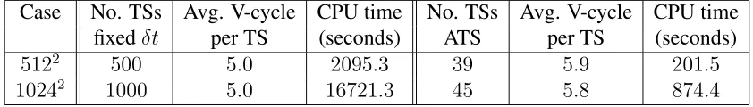
at very early times, the use of our adaptive time stepping approach reduces the number of time steps required to39and45, respectively.

The detailed comparison between the use of fixed time step size and adaptive time stepping is presented in Table 2. In the 5122 _{case, adaptive time stepping takes just}

9.6%of the time taken when fixed time steps are used. This percentage becomes5.2%

V-cycles required per time step in the adaptive case. Note however that the number of V-cycles needed is still independent of the grid size.

Case No. TSs Avg. V-cycle CPU time No. TSs Avg. V-cycle CPU time

fixedδt per TS (seconds) ATS per TS (seconds)

5122 _{500 5.0 2095.3 39 5.9 201.5}

10242 _{1000 5.0 16721.3 45 5.8 874.4}

Table 2: Comparisons between the use of fixed time step size and the adaptive time stepping for two test cases. The total number of time steps, the average V-cycles required per time step and the CPU time are used for the comparisons. Due to the limit of space, abbreviations are used, where TS means “time step”, Avg. means average and ATS is short for adaptive time stepping.

For completeness, two questions are worth asking. Firstly, are our choices of the time step size too small for the fixed time step approach? In other words, could the fixed time step approach take a larger step size and be more competitive? Additional tests show that for the5122 _{case, increasing the initial time step size by a factor of 5}

causes the multigrid solver to converge more slowly as, within each time step, about three more V-cycles are needed. The computation fails to converge if the initial time step size is increased by a factor of10. Thus, the adaptive time-stepping outperforms the fixed time-stepping by a large margin for this specific problem.

The second question is: when using the adaptive time stepping, how accurate are these solutions? Since the exact solution to this problem is not known we choose to base our assessment of the accuracy upon a comparison of the height of the simulated droplets at the centre of the domain (the maximum height of the droplet) as a function of time, as shown in Figure 5. From this figure, it can be seen that by using adaptive time-stepping, the overall evolutions of the height of the droplet are very close to the ones using the original approach with fixed time step sizes. To give a further indication of how accurate the solutions are at the end of simulation, a zoom-in is shown in the right-hand side of Figure 8. The results shown indicate that our adaptive time stepping approach deteriorates the accuracy by only a very small amount. More specifically, for the5122 _{case, the values of the maximum heights of the droplet atT = 10}−₅

are

3.406 from the use of fixed time step size, and 3.403 from the use of adaptive time stepping. For the10242_{case, the value is3.423from the use of fixed time step, and is}

3.419from the use of adaptive time stepping.

This droplet spreading test case is one which is likely to benefit from employing AMR, since the problem features a distinct radial moving contact line which must be accurately resolved, while elsewhere the solution is relatively smooth. To illustrate our AMR strategy, we choose three test cases for the purpose of demonstration. Their finest grids, if refined everywhere, would have resolutions of2562_,5122 _and10242_.

0 0.1 0.2 0.3 0.4 0.5 0.6 0.7 0.8 0.9 1 x 105

3 3.5 4 4.5 5

Time

h

(t

)

256x256 512x512 1024x1024

adaptive time stepping 512x512 adaptive time stepping 1024x1024

9.4 9.5 9.6 9.7 9.8 9.9 10

x 106 3.36

3.38 3.4 3.42 3.44 3.46 3.48

Time

h

(t

)

256x256 512x512 1024x1024

adaptive timestepping 512x512 adaptive timestepping 1024x1024

Figure 8: The left-hand side figure shows the evolution of the maximum height of the droplet in selected cases. Results with the finest grids2562_,5122_and10242_{have been}

previously presented in Figure 5, where they are obtained using the fixed time step size. The right-hand side figure shows a zoom-in for the end of the graphs that are presented in the left-hand side figure.

our adaptive refinement strategy is based upon a discrete approximation to the second derivative of the droplet thickness h (i.e. |∇2_{h|). Within each mesh block, at every}

grid point,(i, j), the adaptive assessment is computed via:

adaptive assessment_i,j =|hi+1,j+hi−1,j+hi,j+1+hi,j−1−4hi,j| ≈dx2|∇2h|i,j. (14)

Each block is then flagged for refinement or coarsening based on the maximum value of adaptive assessment within the block. In this work:

• if adaptive assessment is greater than the threshold: > ctore = 0.01, mark the block for refinement.

• if adaptive assessment is less than the threshold: < ctode = 0.001, mark the block for coarsening.

This choice of thresholds is quite aggressive, so most of the computation is around the moving contact line.

Here we evaluate the AMR on its own, i.e. without using adaptive time-stepping. In Table 3, details of the three different test cases are presented. They are AMR2562_,

AMR5122_{and AMR1024}2_{. For comparison, we also include the CPU times for these}

test cases when uniform grids and fixed time step size are employed. From this table, the efficiency gained from using AMR is demonstrated. For instance, in AMR10242

Cases δt Time steps Avg. V-cycles CPU time CPU time (seconds) per time step (seconds) from uniform grids AMR2562 _4×10−₈

250 5.0 175.1 303.2

AMR5122 _2×10−₈

500 5.0 645.6 2345.7

AMR10242 _1×10−8 _{1000 5.5 3578.9 18521.1}

Table 3: Details of three test cases using aggressive AMR with fixed time steps. CPU times when only using uniform grids are also included for comparison.

Having presented the CPU time, we further compare the number of grid points on the finest grids used in the uniform cases to the number of leaf grid points that are used in the adaptive cases. The leaf grid points are those grid points that are on the finest refinement level present in their local region. Since refining and coarsening are carried out dynamically, these numbers of leaf points are the maximum numbers that occurred throughout each of the simulations. In Table 4, this comparison is summarised. From this table, the computational workload saved by using the AMR compared to the use of uniform grids is seen to be substantial. For example, in the AMR10242 _{case, the}

number of leaf points is less than 1.0% of the number of points on the finest uniform grid.

Cases Maximum No. leaf Total No. grid points Ratio between grid points from uniform grids AMR and uniform grids

AMR2562 _{2,048 65,536 0.0313}

AMR5122 _{6,400 262,144 0.0244}

AMR10242 _{10,240 1,048,576 0.0098}

Table 4: Comparison of the maximum number of leaf grid points used in adaptive test cases and the total number of grid points in uniform test cases. A ratio between the number of leaf points with AMR and the number of grid points with uniform grids is also presented.

We have demonstrated that the use of AMR significantly improves the efficiency of the computation. However, it can be seen from Tables 3 and 4 that the CPU costs do not reduce with the same rate as the number of grid points. This is because, even when the grid points are significantly decreased by using AMR, the number of grid visits is still the same in our multigrid solver. Additionally, overheads occur when we dynamically maintain the parent-children relations between coarsening and refining. Furthermore, since this software is written with parallelization in mind, other extra overheads also exist in the implementation to deal with issues arising from parallel situations, and those overheads also affect the performance when only one CPU is employed, e.g. keeping a well parallelizable ordering of all mesh blocks dynamically during the simulation.

how accurate are the solutions from using the AMR? Once again we use the dis-crepency in the maximum height of the droplet between different simulated solutions as a proxy for the error, comparing AMR results against those obtained using uniform grids. In the left-hand side of Figure 9, the evolutions of the maximum height of the droplet from the three test cases (i.e. AMR 2562_{, AMR 512}2 _{and AMR1024}2_{) with}

the use of AMR are presented. Results from using uniform grids (previously shown in Figure 5) are also presented for comparison. From this figure, we see that the use of the AMR produces almost identical results to the ones from using uniform grids.

Furthermore, to assess this in more detail, a zoom-in is shown on the right-hand side of Figure 9 which focusses on the solution at the end of the simulation, and height values are given in Table 5. Using adaptive grids generally compromises the accuracy, as expected given the enormous reduction in degrees of freedom, and these results demonstrate this. It is important to note however that the accuracy of the10242

solution with AMR is much better than the one from the5122 case with uniform grid (i.e. the maximum height of the droplet is much closer to that computed from the

10242 _{case with a uniform grid). It may also be seen that the solution of the AMR}

2562_{is almost identical to the one from the256}2_{case with uniform grid.}

Cases Maximum height Cases Maximum height

AMR2562 _{3.35971 256}2 _3.35974

AMR5122 _{3.405 512}2 _3.406

AMR10242 _{3.418 1024}2 _3.423

Table 5: Comparison of maximum droplet height values at t = 1×10−5 _{for adapted}

and uniform meshes.

9.4 9.5 9.6 9.7 9.8 9.9 10 x 10−6 3.36

3.38 3.4 3.42 3.44 3.46 3.48

Time

h

(t

)

AMR 256x256 AMR 512x512 AMR 1024x1024 256x256 512x512 1024x1024

0 0.1 0.2 0.3 0.4 0.5 0.6 0.7 0.8 0.9 1

x 10−5

3 3.5 4 4.5 5

Time

h

(t

)

AMR 256x256 AMR 512x512 AMR 1024x1024 256x256 512x512 1024x1024

Figure 9: In the left-hand side figure, the evolution of the maximum height of the droplet is plotted from using both AMR and uniform grids. On the right-hand side, a zoom-in is included to assess the accuracy near the final time.

to the evolution of the solution. Here we present snapshots of the evolution of the mesh refinement during typical simulations. These are shown in Figure 10, where different colours are used to identify different levels of mesh refinement. Results shown in this figure demonstrate the dynamic evolution of AMR during a typical simulation.

Figure 10: Snapshots of the evolution of AMR during a typical simulation. Left-hand side is the AMR att = 0and right-hand side shows the AMR att = 1×10−₅

. Mesh refinement levels:1282_{(dark blue);256}2 _{(light blue);512}2_{(yellow);1024}2 _(red).

The spatial and the temporal discretization schemes that are used in this work are both second-order accurate. Therefore, we expect the overall convergence rate to be second order, i.e. the error behaves as O(δt2_{, dx}2_{) as the mesh is refined. This}

means that halving the time step size and doubling the number of grid points in each direction should reduce the error by a factor of four. Although we do not have an exact solution to compare with, we can still look at differences between solutions at successive levels of refinement: if these also reduce by a factor of four each time δt

anddxare halved then this indicates second order convergence to a solution. In order to illustrate this, we conduct our convergence tests based upon solution restriction. For example, consider three grid hierarchies using 2-D grids: 82 ₋₁₆2_,82₋₃₂2 _and

82−642. Each grid is associated with aδt:δt(162

),δt(322

)=

δt₍162)

2 andδt(642)=

δt₍322)

2 ,

respectively. Solutions are obtained by solving the same problem on these three finest grids separately, with their correspondingδt, and with the assumption that the ending timeT is exactly the same for all runs. To make a comparison between two solutions we restrict the fine grid solution to the coarse grid by using a restriction operator (e.g. four-point averaging shown in Equation (5)). Thus, the solution which is restricted from grid hierarchy 82 _{− 32}2 _{can be compared to the solution from grid hierarchy}

82₋₁₆2_{. Similarly, the restricted solution from hierarchy8}2 ₋₆₄2 _{can be compared}

to the original solution from hierarchy82₋₃₂2_.

are

||e||∞ :=max(|urestricted_i,j −ui,j|), ||e||2 :=

s

PN

i=1

PN

j=1(urestrictedi,j −ui,j)2

N ×N , (15)

whereurestricted_{is the restricted solution from the finer grid hierarchy,uis the solution}

from the coarser grid hierarchy,i, j = 1, . . . , N andN is the number of internal grid points in each axis direction on the finest level of the coarser grid hierarchy. When adaptive grids are used, at the final stage t = T, we transfer the solutions to the uniform meshes that are needed in order to carry out these comparisons.

In Table 6, we present convergence results that are generated using adaptive time-stepping, AMR and parallel computing from four different simulations. Their highest levels of mesh refinement are equivalent to uniform grid resolutions of 5122_{, 1024}2_,

20482 _{and 4096}2 _{respectively. A 16}2 _{coarsest grid is used for all cases. The end}

time is chosen to be T = 2.0×10−2_{, which is longer than the previous ones, and}

constitutes a “full” simulation. Results shown in this table clearly demonstrate second order convergence for both variableshandp.

For variableh

Cases Startingδt Time steps Infinity norm Ratio Two norm Ratio

AMR5122 _1×10−₈

1418 - - -

-AMR10242 _5×10−9 _{2011 2.480×10}−5 _{- 1.117×10}−5

-AMR20482 _2.5×10−9 _{25184 6.174×10}−6 _{4.02 2.737×10}−6 _4.08

AMR40962 _1.25×10−₉

472368 1.544×10−₆

3.99 6.864×10−₇

3.99

For variablep

AMR5122 _1×10−8 _{1418 - - -}

-AMR10242 _5×10−₉

2011 5.321×10−₂

- 2.007×10−₂

-AMR20482 _2.5×10−9 _{25184 1.324×10}−2 _{4.02 4.873×10}−3 _4.12

AMR40962 _1.25×10−9 _{472368 3.309×10}−3 _{3.99 1.208×10}−3 _4.04

Table 6: Results show the differences in consecutive solutions measured in the stated norm, followed by the ratio of consecutive differences from the droplet spreading model with the initial condition given in Equation (12). These results are generated with solutions atT = 2.0×10−2_{using spatial and temporal adaptivity.}

3.2

A Multi-Phase-Field Model of Tumour Growth

In the previous section we illustrated the performance of our software for a 2-dimensional mathematical model of thin film flow. In this section we consider an even more com-plex test problem, with a greater number of nonlinear PDEs and in both two and three space dimensions.

model the morphology of tumours. The review papers [27, 28, 29] describe a number of examples of how such models can be derived. In the work presented here, a multi-phase-field model of tumour growth is considered, from Wise et al. [3]

There are, in total, four independent phase-field variables in this model, namely

φW, φH, φV and φD, which represent volume fractions of extracellular fluid, healthy

cells, viable tumour cells and dead tumour cells, respectively. In addition, there are three assumptions applied to these volume fractions.

1. The extracellular fluid volume fraction is everywhere constant, i.e.φW(x, y, z, t) = φW,0 =constant.

2. Cells are assumed to be close-packed, soφH +φV +φD = 1, and the range of

values of these phase-field variables is from0to1.

3. Inside the tumour there are only two types of cells: viable and dead. This indi-cates the total tumour cell volume fraction isφT =φV +φD.

Based upon these three assumptions, there are only two phase-field variables that are required to be solved, and they areφT andφD. Once these two variables are obtained,

other variables may be derived from the assumptions made.

The componentφT is assumed to obey the following Cahn-Hilliard-type

advection-reaction-diffusion equations:

∂φT

∂t =M∇ ·(φT∇µ) +ST − ∇ ·(uSφT), (16)

µ=f′

(φT)−ǫ2∇2φT, (17)

whereM > 0is the mobility constant,f(φT) =φ2T(1−φT)2/4is the quartic

double-well potential,uS is the tissue velocity (which is substituted for using Equation (23)),

andǫ > 0is an interface thickness parameter between healthy and tumour tissue. ST

is the net source of tumour cells, and is given as

ST =nG(φT)φV −λLφD, (18)

where n is the concentration of nutrient, which is specified in Equation (26), φV = φT −φD, andλL ≥ 0is the rate of tumour cell proliferation. G(φT)is a continuous

cut-off function defined as

G(φT) =







1 if 3₂ǫ ≤φT φT

ǫ −

1

2 if

ǫ

2 ≤φT < 3ǫ

2

0 ifφT < ǫ₂.

(19)

A similar dynamical equation for predicting the volume fraction of dead tumour cellsφD is used:

∂φD

whereSD is the net source of dead tumour cells, defined as

SD = (λA+λNH(nN −n))φV −λLφD, (21)

where λA is the death rate of tumour cells from apoptosis, λN is the death rate of

tumour cells from necrosis, nN is the necrotic limit (necrosis only occurs when the

nutrient value is below this limit), and H is a Heaviside function. This Heaviside function is discontinuous and thus could prevent us from obtaining a higher order convergence rate, so we instead use the smoother approximation given by

H(nN −n) =







1 ifnN −n ≥ǫs

−_4(ǫ1s₎3 (nN −n) 3

+ ₄3_ǫs (nN −n) +

1

2 if−ǫ

s _≤n

N −n ≤ǫs

0 ifnN −n <−ǫs,

(22) whereǫs_{controls the steepness of the smooth transition between0and1.}

The tissue velocityuS is assumed to obey Darcy’s law, and is defined as

uS =−κ(φT, φD)(∇p−

γ

ǫµ∇φT), (23)

where κ(φT, φD) > 0 is the tissue motility function and γ ≥ 0 is a measure of the

excess adhesion. An additional assumption made by Wise et al. [3] is that there is no proliferation or death of the host tissue, thus the velocity is constrained to satisfy

∇ ·uS =ST. (24)

Instead of solving for the tissue velocity, Equations (23) and (24) are combined to-gether, and a Poisson-like equation for the cell pressurepcan be constructed:

−∇ ·(κ(φT, φD)∇p) =ST − ∇ ·(κ(φT, φD) γ

ǫµ∇φT). (25)

A quasi-steady equation is given for the nutrient concentration through diffusion:

0 =∇ ·(D(φT)∇n) +Tc(φT, n)−n(φT −φD), (26)

where

D(φT) = DH(1−Q(φT)) +Q(φT) (27)

is the diffusion coefficient, DH is the nutrient diffusivity in the healthy tissue,Q(φT)

is an interpolation function, given by

Q(φT) =







1 if1≤φT 3φ2

T −2φ3T if0< φT <1

0 ifφT ≤0.

(28)

and

is the nutrient capillary source term. Furthermore, vH

P ≥ 0 and vPT ≥ 0 are

con-stants specifying the degree of pre-existing uniform vascularization, and nC ≥ 0 is

the nutrient level in capillaries.

To sum up, this multi-phase-field model of tumour growth consists of a coupled system made up of Equations (16), (17), (20), (25) and (26). There are five dependent variables in total in this system: two phase-field variables, φT and φD; and three

supplementary variables, µ, pandn. These PDEs are valid throughout a domainΩ, and there are no internal boundary conditions for the solid tumour, the necrotic core or other variables. Therefore, only one set of outer boundary conditions is required (provided the tumour is in the domain’s interior) and this set is the following mixture of Neumann and Dirichlet boundary conditions:

µ=p= 0, n= 1, ∂φT

∂ν =

∂φD

∂ν = 0 on ∂Ω, (30)

whereνdenotes the outward-pointing normal direction to the boundary∂Ω.

We discretise all of the derivatives (including those of odd order) in this model using second order centred differences. This approximation may introduce spurious numerical oscillations in the vicinity of steep fronts which could lead to unphysical values for the phase volume fractions. In order to retain the expected second order convergence rate while forcing the phase volume fractions to lie between 0 and 1 (or very close to that interval) additional penalty terms are added to Equations (16) and (20), which take the form

1

δmin (φT,0) and

1

δmax (φT −1,0) (31)

for φT, with a corresponding term added to the φD equation. These terms have no

impact when 0≤ φ ≤ 1, but create a large correction to the system wheneverφtries to take a value outside of this interval. The smaller the choice of the penalty parameter

δ(i.e. the larger1/δ) the larger this correction becomes, forcing the values ofφto be close to this range but at the expense of adding to the nonlinearity of the resulting system. The default value of δ used in this work is 10−4_{. This is a slightly more}

relaxed constraint on the range of values that can be taken by φD and φT than that

imposed by Wise et al. [3], who enforced φ∈[0,1]in a non-smooth manner.

In order to define the initial conditions for the 2-D simulations, firstly the 2-D domain Ωis given by (x, y) ∈ Ω = [0,40]×[0,40]. An initial condition for φT is

defined to be

φT(x, y) =1 if

(x−20)2

1.1 + (y−20)

2 _≤22_,

=0 otherwise.

(32)

This initial condition is discontinuous, so we employed a simple Jacobi iteration with