Multi exposure laser speckle contrast imaging using a high frame rate CMOS sensor with a field programmable gate array

See discussions, stats, and author profiles for this publication at: https://www.researchgate.net/publication/282429234

Multi-exposure laser speckle contrast imaging

using a high frame rate CMOS sensor with a field

programmable gate array

Article in Optics Letters · October 2015 DOI: 10.1364/OL.40.004587

CITATIONS

3

READS

107

5 authors, including:

Some of the authors of this publication are also working on these related projects:

Multidisciplinary Assessment of Technology Centre for Healthcare 2003-2013 - various projectsView project

Acoustics of biomaterialsView project Yiqun Zhu

University of Nottingham 20PUBLICATIONS 158CITATIONS

SEE PROFILE

Stephen P Morgan

University of Nottingham 149PUBLICATIONS 1,108CITATIONS

SEE PROFILE

All content following this page was uploaded by Stephen P Morgan on 07 October 2015.

Multi-Exposure Laser Speckle Contrast Imaging

using a High Frame Rate CMOS Sensor with a

Field Programmable Gate Array

Shen Sun,1 Barrie R Hayes-Gill,1 Diwei He,1 Yiqun Zhu,1 and Stephen P Morgan1,* 1

Advanced Optics Group, Faculty of Engineering, University of Nottingham, Nottingham, UK, NG7 2RD

*Corresponding author: [email protected]

Received Month X, XXXX; revised Month X, XXXX; accepted Month X, XXXX; posted Month X, XXXX (Doc. ID XXXXX); published Month X, XXXX

A system has been developed in which multi-exposure Laser Speckle Contrast Imaging (LSCI) is implemented using a high frame rate CMOS imaging sensor chip. Processing is performed using a Field Programmable Gate Array (FPGA). The system allows different exposure times to be simulated by accumulating a number of short exposures. This has the advantage that the image acquisition time is limited by the maximum exposure time and that regulation of the illuminating light level is not required. This high frame rate camera has also been deployed to implement laser Doppler blood flow processing enabling direct comparison of multi-exposure laser speckle contrast imaging and Laser Doppler Imaging (LDI) to be carried out using the same experimental data. Results from a rotating diffuser indicate that both multi-exposure LSCI and LDI provide a linear response to changes in velocity. This cannot be obtained using single-exposure LSCI unless an appropriate model is used for correcting the response. © 2015 Optical Society of America

OCIS Codes: (030.6140) Speckle, (120.3890) Medical optics instrumentation, (120.6150) Speckle imaging, (170.3340) Laser Doppler velocimetry.

http://dx.doi.org/xxxxxxxxxxxx

Laser speckle contrast imaging (LSCI) is widely applied in blood flow measurements in the microcirculation [1]. However, in comparison to laser Doppler imaging (LDI) [2]-[5], LSCI does not provide a linear relationship between blood flow and contrast [6]. One of the reasons is the presence of static speckle in the image caused by scattering of light from static tissue [6]. To address this problem multi-exposure LSCI (MLSCI) has been developed in which

the intensity of the speckle pattern (𝐾) is measured

over a range of exposure times and this can be

related to blood flow via the correlation time 𝜏𝑐 using

a relationship of the form [6],

𝐾(𝑇, 𝜏𝐶) = {𝛽𝜌2

𝑒−2𝑥_{− 1 + 2𝑥}

2𝑥2 + 4𝛽𝜌(1 − 𝜌)

𝑒−𝑥_{− 1 + 𝑥}

𝑥2

+ 𝑣𝑛𝑒+ 𝑣𝑛𝑜𝑖𝑠𝑒}

1 2

(1) 

where 𝜌 accounts for the presence of light scattered by

static tissue, 𝛽 accounts for the speckle averaging effect.

𝑣𝑛𝑒 represents the constant variance due to non-ergodic

light, and 𝑣𝑛𝑜𝑖𝑠𝑒 is the experimental noise. 𝑥 is the ratio of

exposure time to correlation time (𝑇/𝜏𝑐).

Several authors have presented different MLSCI algorithms for providing more accurate measurement of blood flow, a reduction of the effects of scattering from static tissue and a linear relationship between contrast and blood flow [7]-[9]. One of the drawbacks of using a multi-exposure approach is that the intensity of the illumination needs to be regulated over a wide range of exposure times which makes the system setup more

complicated [6]-[9]. In addition as a series of images needs to be acquired sequentially, image acquisition time increases to the total acquisition time of all images. Here we present a novel MLSCI system using a high-speed CMOS imaging sensor linked to a field programmable gate array (FPGA). This arrangement allows the data to be acquired at a high frame rate and processed in parallel. The advantage of this approach compared to previous work [6]-[9] is that acquiring the data at high frame rates allows different exposure times to be simulated by summing the signals obtained at each short exposure. Although different exposure times are simulated by summing the intensities on the FPGA, the actual exposure time of the camera remains constant and so the illumination can remain constant over 3 decades of exposure times throughout the blood flow image acquisition. As all exposure times are acquired simultaneously the blood flow image acquisition time is limited by the longest exposure time, rather than the sum of all exposure times. A similar approach based on a single photon avalanche diode (SPAD) array detector has recently been developed in parallel to this work [10]. Although SPAD arrays remove readout noise, they are, to date, limited by the number of pixels in the array. There are advantages in utilizing megapixel commercial CMOS sensors for high spatial resolution blood flow imaging. Furthermore the FPGA allows for implementation of multiple processing algorithms in parallel, enabling a direct comparison of MLSCI, single exposure LSCI and LDI for the first time.

The system schematic is shown in Fig.1. A high

Xilinx) via a custom-made digital interface. The sensor driver (for controlling the CMOS sensor and timing the image acquisition process) and the contrast processing algorithm are implemented on the FPGA device along with other control logic (i.e., RAM controller, serial controller, PCIe controller). Other peripherals, such as serial interface (RS232), DDR3 SDRAM and PCIe interface, interface with the FPGA to fulfill other functionalities including configuration, raw data storage and data transmission.

Fig. 1. System schematic showing the main imaging, storage, processing and control units. The CMOS sensor interfaces to the FPGA through the FMC socket. Several units including camera controller, memory controller, processing unit, Block Ram, RS232 controller and PCIex8 controller are implemented on the FPGA for driving the camera chip, dispatching data for DDR3 SDRAM, calculating speckle contrast (K), temporarily storing data, configuration and data transmission. K is sent to a PC through the PCIex8 for further processing and display.

Speckle images are continuously captured at a frame rate of 15kHz with a fixed exposure time of 66.7μs. 1024 frames are used to produce one velocity (correlation time) map. Several short exposure frames (66.7μs) can be accumulated to simulate longer exposure times (e.g. 32 frames – 2.1ms, 1024 frames – 68.3ms). An important point to note for the simulation of different exposure times is that the CMOS sensor is built with a pipeline structure which enables the exposure and read out to be conducted simultaneously. This means that any two adjacent frames can be considered as continuously exposed and the time interval between successive exposures (Δt, in the range of 20ns - 1μs) is much smaller than

the intensity correlation time (𝜏𝑐 is typically ~0.1ms

for moving red blood cells).

The speckle model used in the processing algorithm is based on Eq.1. To simplify the fitting

procedure, the 𝛽𝜌2 _{term is merged into one fitting}

parameter, a, 4𝛽𝜌(1 − 𝜌) is merged into parameter b,

and 𝑣𝑛𝑒and 𝑣𝑛𝑜𝑖𝑠𝑒 are combined into one parameter 𝑐.

The simplified modified speckle model used is,

𝐾(𝑇, 𝜏𝑐) = {𝑎

𝑒−2𝑥_{− 1 + 2𝑥}

2𝑥2 + 𝑏

𝑒−𝑥_{− 1 + 𝑥}

𝑥2

+ 𝑐}

1 2

(2)

Parameters a, b, c and the correlation time (𝜏𝑐) are

then found by fitting a set of multi-exposed contrast values using the least squares method. It is worth noting that the summation of multiple short exposures produces a similar signal level to conventional MLSCI but the noise is proportional to sum of the square roots of each exposure time. This will introduce an error when applying the speckle model (Eq.2) but the results presented demonstrate that in practice this is not a significant effect.

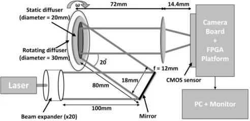
Fig. 2. Experimental setup for the rotating diffuser test. A green laser beam is expanded to a diameter of 18mm and illuminates a static diffuser at an angle of 20 degrees. A white rotating cardboard disc (diameter 30mm) is placed behind the diffuser to simulate moving red blood cells. A region of 18mm×18mm square is imaged onto 320×320 pixels of the CMOS sensor.

In order to evaluate the MLSCI system, a rotating diffuser lying behind a static diffuser provides a controlled sample that acts as a tissue phantom [11], [12] for moving red blood cells flowing underneath a static layer of skin. This generates flow profiles that can be controlled through the motor drive voltage and which change linearly with radial position on the diffuser. A green laser beam (OXXIUS S.A. 532

S-50-COL-PP, wavelength 𝜆 = 532nm, Power = 50mW) is

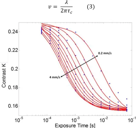
diffuser on the CMOS camera chip with a magnification of 0.2. A region of 18mm×18mm square is imaged onto 320×320 pixels on the CMOS sensor. This image size is limited by the laser power and can be increased by using higher laser power. The diffuser rotates from 0.05rad/s up to 0.95rad/s which corresponds to a linear velocity of 0.2mm/s to 4mm/s (0.44mm/s incremental step size) at a position r = 4.2mm (central velocity) on the diffuser. The contrast values corresponding to different velocities and different exposure times are shown in Fig.3 along with the least squares fit of Eq.2 to the measured data. The correlation time can then be used to estimate the flow velocity [13]:

𝑣 = 𝜆

2𝜋𝜏𝑐 (3)

Fig. 3. Contrast-exposure time curves. Contrast values were obtained at exposure times of 66.7μs, 133.4μs, 266.8μs, 533.6μs, 1.1ms, 2.1ms, 4.3ms, 8.5ms, 17.1ms, 34.2ms and 68.3ms. These were used to obtain the correlation time at different linear velocities of 0.2mm/s, 0.44mm/s, 0.88mm/s, 1.33mm/s, 1.78mm/s, 2.22mm/s, 2.67mm/s, 3.11mm/s, 3.56mm/s and 4.0mm/s.

The range of velocities covers that which might typically be observed in the microcirculation [14]. In LDI this corresponds to a frequency spectrum of 20Hz to 20kHz [14] which corresponds to exposure times from 25μs to 25ms for MLSCI. Fig.4 displays the velocity profile calculated from the correlation

time (𝜏𝑐) using Eq.3. The response is linear but is a

factor of ~10 less than the actual velocity. This indicates limitations in the application of Eq.3 and the inability of the MLSCI system to directly measure the absolute velocity values due to the statistical uncertainties of the velocity model (e.g. the shape of the scatterers, complex velocity distributions within the object) [15], [16]. However this can be compensated with calibration.

Fig. 4. Velocity calculated from the estimated correlation time after repeating the experiment 16 times. The response is linear (𝑦 = 0.11𝑥 − 0.009 using least square fit) but is underestimated by a factor of approximately 10.

An additional benefit of the system is that the high frame rate sensor provides a wide bandwidth (up to 7.5kHz) which can be used to provide laser Doppler imaging (LDI) [17]. It should be noted that a bandwidth of up to 20KHz is usually used in laser Doppler imaging and that this is implemented using either a scanning system [18] or a custom made sensor [11], [12]. However much of the power spectrum is concentrated at lower frequencies and so a high frame rate sensor often provides an adequate approximation. Introducing LDI signal processing onto the FPGA [18] enables direct comparison of MLSCI and LDI using the same experimental data. LDI processing is implemented by taking the Fourier transform of 1024 samples acquired and then frequency weighting the power spectrum [16]. The

mean beat frequency (𝑓̅) is calculated by the

normalized first moment [16], [19], which can be used to obtain the mean velocity by,

|𝑣̅| = 𝑓̅ × 𝜆 (4)

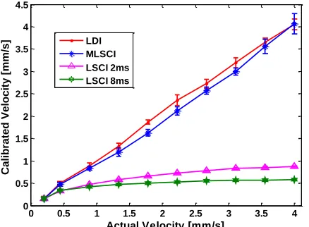
Eq.2 and Eq.4 allow a direct comparison of LDI and MLSCI. The results shown in Fig.5 were calibrated relative to the known velocity at 0.2mm/s [16]. For reference, LSCI velocity values at 2 fixed exposure times are also shown which are obtained by accumulating a certain amount of frames (30 frames for ~2ms, and 120 frames for ~8ms). This demonstrates the non-linearity of LSCI compared to MLSCI and LDI and a detailed study will be the subject of a future paper.

Previously demonstrated MLSCI methods based on CMOS sensors suffer from reduced imaging frame rate as it is set by the sum of all exposure times [6], [8]. In the method described here, the frame rate is

0 1 2 3 4

0 0.1 0.2 0.3 0.4 0.5

Actual Velocity (mm/s)

M

e

a

s

u

re

d

V

e

lo

c

it

y

(

m

m

/s

set by the maximum exposure time. The image acquisition time is 68.3ms which would increase to ~137ms for the sequential imaging case in the experiments conducted. The approach is particularly beneficial for practical implementation as the system can utilize a constant illumination level, with a 3-decade range of exposure times (66.7µs – 68.3ms) being obtained at a temporal resolution of 66.7µs.

Fig. 5. Calibrated velocity profiles of MLSCI, LDI and conventional LSCI using 2 fixed exposure times. The error bars are obtained from the standard deviation of the measured velocity obtained 16 times.

This CMOS imaging sensor and adjacent FPGA provide a flexible approach for implementing the signal processing with blood flow and velocity being obtained using MLSCI, single-exposure LSCI and LDI processing. The results obtained from a spinning diffuser have demonstrated a linear relationship between actual velocity and calculated velocity for both LDI and MLSCI. Although the earlier assertion made by Briers [20] that LDI and LSCI are effectively identical and interchangeable is not supported for single exposure LSCI (Fig.5) It has been demonstrated using the same experimental data that MLSCI, provides a response comparable to LDI but with the advantage of simpler signal processing implementation. The MLSCI system presented here is promising for imaging blood flow as full field LDI has been widely demonstrated using similar exposure times [11], [17].

Acknowledgement

This work was partially supported by an Engineering and Physical Sciences (EPSRC) UK Knowledge Transfer Secondment.

References

1. D.A. Boas and A.K. Dunn, J. Biomed. Opt.

15(1):011109 (2010).

2. K. R. Forrester, C. Stewart, J. Tulip, C. Leonard

and R.C. Bray, Med. Biol. Eng. Comput. 40.6, 687 (2002).

3. A. T. Garry, M. Klonizakis, H. Crank, J.D.

Briers and G.J. Hodges, Microvasc. Res. 82.3, 326 (2011).

4. A. Humeau-Heurtier, G. Mahe, S. Durand and

P. Abraham, Opt. Commun. 291, 483 (2013).

5. O. Thompson, J. Bakker, C. Kloeze, E.

Hondebrink and W. Steenbergen, Proc. SPIE 8222, Dynamics and Fluctuations in Biomedical Photonics IX 822204 (2012).

6. A.B. Parthasarathy, W.J. Tom, A. Gopal, X.

Zhang and A.K. Dunn, Opt. Express 16.3, 1975 (2008).

7. P. Zakharov, A.C. Völker, M.T. Wyss, F. Haiss,

N. Calcinaghi, C. Zunzunegui, A. Buck, F. Scheffold and B. Weber, Opt. Express 17.16, 13904 (2009).

8. T. Smausz, D. Zölei and B. Hopp, Appl. Opt.

48.8, 1425 (2009).

9. O.B. Thompson and M.K. Andrews, J. Biomed.

Opt. 15.2, 027015 (2010).

10. T. Dragojević, D. Bronzi, H. Varma, C. Valdes, C.

Castellvi, F. Villa, A. Tosi, C. Justicia, F. Zappa, and T. Durduran, Biomed. Opt. Express 6, 2865-2876 (2015).

11. D. He, H.C. Nguyen, B.R. Hayes-Gill, Y. Zhu,

J.A. Crowe, G.F. Clough, C.A. Gill and S.P. Morgan, Opt. Lett. 37.15, 3060 (2012).

12. D. He, H.C. Nguyen, B.R. Hayes-Gill, Y. Zhu,

J.A. Crowe, C. Gill and S.P. Morgan, Sensors 13(9), 12632 (2013).

13. J.D. Briers, S. Webster, Opt. Commun. 116.1,

36-42 (1995).

14. G. V. Belcaro, U. Hoffmann, A. Bollinger and

A.N. Nicolaides, Laser, Med-orion Publishing Company, pp.293, ISBN: 9963-592-53-8.

15. M. Draijer, E. Hondebrink, T.V. Leeuwen and

W. Steenbergen, Laser Med. Sci. 24.4, 639 (2009).

16. J.D. Briers, Physiol. Meas. 22.4, R35 (2001).

17. A. Serov and T. Lasser, Opt. Express 13.17,

6416 (2005).

18. H.C. Nguyen, B.R. Hayes-Gill, S.P. Morgan, Y.

Zhu, D. Boggett, X. Huang and M. Potter, J. Med. Eng. Technol. 34.5-6, 306 (2010).

19. R. Bonner and R. Nossal, Appl. Opt. 12.20, 2097

(1981).

20. J.D. Briers, J.Opt. Soc. Am. A 13.2, 345 (1996).

0 0.5 1 1.5 2 2.5 3 3.5 4

0 0.5 1 1.5 2 2.5 3 3.5 4 4.5

Actual Velocity [mm/s]

Calib

rated

Vel

ocity

[mm/

s] LDI

References

1. Boas, D.A. and Dunn, A.K., (2010) Laser speckle

contrast imaging in biomedical optics, J. Biomed. Opt. 15(1):011109.

2. Forrester, K. R., Stewart, C., Tulip, J., Leonard,

C., and Bray, R.C., (2002), Comparison of laser speckle and laser Doppler perfusion imaging: measurement in human skin and rabbit articular tissue, Med. Biol. Eng. Comput., 40.6 (2002): 687-697.

3. Garry, A. T., Klonizakis, M., Crank, H., Briers,

J.D., and Hodges, G.J., (2011), Comparison of laser speckle contrast imaging with laser Doppler for assessing microvascular function, Microvascular Research, 82.3 (2011): 326 – 332.

4. Humeau-Heurtier, A., Mahe, G., Durand, S., and

Abraham, P., (2013), Skin perfusion evaluation between laser speckle contrast imaging and

laser Doppler flowmetry, Optics

Communications, 291 (2013): 483 – 487.

5. Thompson, O., Bakker, J., Kloeze, C.,

Hondebrink, E., and Steenbergen, W., (2012), Experimental comparison of perfusion imaging systems using multi-exposure laser speckle, single-exposure laser speckle, and full-field laser Doppler, Proc. SPIE 8222, Dynamics and Fluctuations in Biomedical Photonics IX, 822204 (February 9, 2012).

6. Parthasarathy, A. B., Tom, W. J., Gopal, A.,

Zhang, X., and Dunn, A. K., (2008), Robust flow measurement with multi-exposure speckle imaging, Opt. Express, 16.3 (2008): 1975-1989.

7. Zakharov, P., Völker, A. C., Wyss, M. T., Haiss,

F., Calcinaghi, N., Zunzunegui, C., Buck, A., Scheffold, F., and Weber, B., (2009), Dynamic laser speckle imaging of cerebral blood flow, Opt. Express, 17.16 (2009): 13904-13917.

8. Smausz, T., Zölei, D., and Hopp, B., (2009), Real

correlation time measurement in laser speckle contrast analysis using wide exposure time range images, Applied optics, 48.8 (2009): 1425-1429.

9. Thompson, O. B., and Andrews, M. K., (2010),

Tissue perfusion measurements: multiple-exposure laser speckle analysis generates laser

Doppler-like spectra, SPIE, Journal of

Biomedical Optics, 15.2 (2010): 027015-027015.

10. Dragojević, T., Bronzi, D., Varma, H., Valdes, C.,

Castellvi, C., Villa, F., Tosi, A., Justicia, C., Zappa, F., and Durduran, T., (2015), High-speed multi-exposure laser speckle contrast imaging with a single-photon counting camera, Biomed. Opt. Express 6 (2015), 2865-2876.

11. He, D., Nguyen, H.C., Hayes-Gill, B.R., Zhu, Y.,

Crowe, J.A., Clough, G.F., Gill, C.A., and

Morgan, S.P., (2012), 64×64 pixel smart sensor array for laser Doppler blood flow imaging, Opt Lett., 37.15 (2012): 3060-3062.

12. He, D., Nguyen, H. C., Hayes-Gill, B. R., Zhu, Y.,

Crowe, J. A., Gill, C., Clough, G.F. and Morgan, S. P. (2013), Laser doppler blood flow imaging using a cmos imaging sensor with on-chip signal processing. Sensors, 13.9 (2013), 12632-12647.

13. Briers, J. D., and Webster, S., (1995), Quasi-real

time digital version of single-exposure speckle photography for full-field monitoring of velocity or flow fields, Opt. Commun., 116.1 (1995): 36-42.

14. Belcaro, G. V., Hoffmann, U., Bollinger, A., and

Nicolaides, A.N., (1994), Laser Doppler, Med-orion Publishing Company, pp. 293, ISBN: 9963-592-53-8.

15. Draijer, M., Hondebrink, E., Leeuwen, T.v., and

Steenbergen, W., (2009), Review of laser speckle contrast techniques for visualizing tissue perfusion, Lasers in Medical Science, 24.4 (2009): 639-651.

16. Briers, J. D., (2001), Laser Doppler, speckle and

related techniques for blood perfusion mapping and imaging, Physiol. Meas., 22.4 (2001): R35.

17. Serov, A., & Lasser, T. (2005), High-speed laser

Doppler perfusion imaging using an integrating CMOS image sensor. Optics Express, 13.17 (2005), 6416-6428.

18. Nguyen, H. C., Hayes-Gill, B. R., Morgan, S. P.,

Zhu, Y., Boggett, D., Huang, X., and Potter, M., (2010), A Field-Programmable Gate Array Based System for High Frame Rate Laser Doppler Blood Flow Imaging: J Med Eng Technol, 34.5-6 (2010): 306-315.

19. Bonner, R., and Nossal, R., (1981), Model for

laser Doppler measurements of blood flow in tissue, OSA, Appl. Opt., 12.20 (1981): 2097-2107.

20. Briers, J. D., (1996), Laser Doppler and

time-varying speckle: a reconciliation, J.Opt. Soc. Am. A, 13.2 (1996): 345-350.