Full metadata for this item is available in Research@StAndrews:FullText at:
http://research-repository.st-andrews.ac.uk/
Interest rate rules and welfare in open economies
Ozge Senay
Date of deposit 09/02/2012
Version This is an author version of this work.
Access rights © This item is protected by original copyright.
This work is made available online in accordance with publisher policies. To see the final definitive version of this paper please visit the publisher’s website.
Citation for
published version Senay, O. (2008). Interest rate rules and welfare in openeconomies. Scottish Journal of Political Economy, 55(3): pp300-329.
Link to published
Interest Rate Rules and Welfare in Open Economies
Ozge Senay
∗Scool of Economics and Finance
University of St Andrews
†October 1, 2007
Abstract
This paper analyses the welfare performance of a set of five alternative interest rate rules in an open economy stochastic dynamic general equilibrium model with nominal rigidities. A rule with a lagged interest rate term, high feedback on infl a-tion and low feedback on output is found to yield the highest welfare for a small open economy. This result is robust across different degrees of openness, different sources of home and foreign shocks, alternative foreign monetary rules and different specifications for price setting behaviour. The same rule emerges as both the Nash and cooperative equilibria in a two-country version of the model.
Keywords: Welfare, Monetary Policy, Interest Rate Rules, Second Order Ap-proximation
JEL: E52, E58, F41
∗I am grateful for useful comments and suggestions from an anonymous referee and the editors.
†Scool of Economics and Finance, University of St Andrews, St Andrews, KY16 9AL. Tel:+44 1334
1
Introduction
Recent research on monetary policy has focused on the use of interest rate rules in which
the nominal interest rate is adjusted in response to economic conditions. A rule proposed
by Taylor (1993) to act as a guide for policymakers setting short-run interest rates has
especially attracted widespread interest. “Taylor rules” in general specify that the
short-run interest rate should be altered in response to an increase in inflation and/or a fall in
real output below targeted levels.1 The collection of papers in Taylor (1999a) provide a
sample of the different variations on the benchmark Taylor rule analysed in many papers.
Indeed, in his introduction to this volume, Taylor (1999a) suggests that the set of rules
used by different authors in the volume is “representative of the degree of disagreement”
among researchers. Taylor (1999a) is regarded as a central reference within the literature
on monetary policy rules.
In common with much research on monetary policy rules, the papers in the Taylor
(1999a) volume are mostly focused on closed economy models.2 However, open economy
issues such as the behaviour of exchange rates and the importance of the exchange rate as
a key transmission mechanism of monetary policy, especially in transmitting the effects of
external shocks, are central to monetary policy. Thus, it is essential to extend the closed
economy literature on monetary rules to an open economy framework.
The objective of this paper is to extend the closed economy analysis of monetary policy
rules, as exemplified by the papers of the Taylor volume, to a general open economy
set-ting. A sticky-price general equilibrium model of an open economy is used to evaluate the
relative welfare performance of the set of interest rate rules examined in the nine different
papers in the Taylor (1999a) volume. The model used draws on the open economy models
1See Clarida, Gali and Gertler (1999), Taylor(1999a) and the June 1999 special issue of theJournal
of Monetary Economics.
2Only two of the nine papers in the Taylor volume consider open economy models (Ball (1999) and
Batini and Haldane (1999)). In both these papers the models used are linear structures which do not
incorporate explicit microeconomic foundations nor do they consider welfare in terms of the utility of a
of Obstfeld and Rogoff (1995, 1998) and the closed economy models of Rotemberg and
Woodford (1997, 1999).3 This framework is useful for formulating an explicit welfare
eval-uation of each policy rule using the utility function of the representative agent. Nominal
rigidities are introduced in the form of Calvo (1983) price contracts which prevent agents
from changing prices in every period in response to domestic and foreign disturbances.
The model incorporates home bias in consumption, thereby allowing a comparison of rules
under different degrees of economic openness. The home country is subject to stochastic
shocks from internal and external sources and the focus of interest is on the stabilisation
and welfare implications of the policy rule choice for the home country.
The welfare performance of the different rules is measured using aggregate utility of
home agents. In this respect, the paper builds directly on the closed economy analysis
of Rotemberg and Woodford (1997 and 1999, which is one of the Taylor (1999a) papers).
This paper makes use of the solution technique developed by Sutherland (2002) to
calcu-late aggregate utility for the comparison of the performance of each of the interest-rate
rules. The explicit evaluation enabled by the utility-based welfare measure will enable a
rigorous comparison of the welfare performances of different rules.
Before proceeding, it is useful to discuss the relationship between the model used in
this paper and the models used in the recent open economy literature. The use of
micro-founded general equilibrium models and utility based welfare measures have, of course,
become more standard in recent years. However, within an open economy context many
of the recent contributions are only able to obtain results in heavily constrained special
cases.4 The results emphasised in this recent literature cannot therefore be regarded as
3King and Wolman (1999), McCallum and Nelson (1999) and Rotemberg and Woodford (1999) are
the main papers in the Taylor (1999a) volume which motivate this study. These models are all closed
economy, optimising, dynamic stochastic general equilibrium models with representative agents having
rational expectations. They also incorporate some form of nominal rigidity in their analyses, through
staggered wage or price setting, which imply some trade-offin inflation and output in the short run. 4This is because the analysis of aggregate utility within an open economy model is technically much
definitive. This is true for instance for the papers by Obstfeld and Rogoff(2002), Clarida,
Gali and Gertler (2002), Gali and Monacelli (2005), Devereux and Engel (2003), Corsetti
and Pesenti (2004) and Benigno and Benigno (2003). All these authors examine cases
where key parameter values, such as the intra- and intertemporal elasticities of
substitu-tion, are restricted to specific values. While these authors are able to obtain interesting
and clear-cut results relating to the welfare effects of monetary policy, it is important to
note that these results are only valid for specific parameter combinations. The results
are not valid for more general parameter combinations. By using second-order
approxi-mation techniques the analysis in this paper considers the general case with unrestricted
parameter values. This implies that intuitions based on results of the papers cited above
cannot be applied directly to the model of this paper. Thus, for instance, the optimality
of price stabilisation which is emphasised by a number of the above authors, depends
crucially on the parameter restrictions imposed in their models. It does not follow that
price stabilisation is optimal in the model of this paper.5
There are some recent papers analysing Taylor rules using models which are not subject
to the above described parameter restrictions. Bergin, Shin and Tchakarov (2005) and
developed by Sutherland (2002), and also by Sims (2000) and Schmitt-Grohe and Uribe (2004). It is
important to note that, while Woodford (2003) and Rotemberg and Woodford (1999) also use
second-order approximations to analyse welfare, the techniques they use are only appropriate for closed economy
settings (or heavily restricted open economy settings). It is only the recently developed second-order
techniques (which are used in this paper) that are more generally applicable.
5Sutherland (2006), who analyses the general case in a static open economy model, has shown that
price stabilisation is only optimal in the special cases analysed in many of the above mentioned papers.
Other recent contributions in the closed and open economy literature have also questioned the optimality
of price stabilisation. For instance, again using second-order approximation techniques, Benigno and
Woodford (2004) have shown that price stabilisation is not optimal when there are shocks to government
spending. Benigno (2001) and Devereux (2004) have shown that price stabilisation is not optimal when
internationalfinancial markets are incomplete. Sutherland’s (2004) results show that price stabilisation
is not a Nash equilibrium of non-coordinated monetary policy in a two-country world (except in the cases
Kollmann (2002) have made use of second-order approximation techniques to investigate
the welfare effects of monetary policy rules. But these authors do not analyse the set
of rules considered in the Taylor (1999a) volume and they restrict attention to simple
Taylor rules without terms in the lagged interest rate. The results of this paper show that
rules including the lagged interest rate can perform significantly better in welfare terms.
Batini, Haldane and Millard (2003) also analyse Taylor rules in a general model but their
measure of welfare does not make use of a full second-order approximation.6
The paper initially focuses on a model which is widely accepted as a benchmark in the
recent open economy macroeconomics literature (see for instance Benigno and Benigno
(2003), Clarida, Gali and Gertler (2002), Gali and Monacelli (2005), Kirsanova, Leith
and Wren-Lewis (2006)).7 At its most basic level the model incorporates sticky prices in
the form of Calvo (1983) contracts where prices are set in the currency of the producer.
Closed economy models of this general type have been subject to quite extensive
estima-tion and empirical testing (see for instance Rotemberg and Woodford (1997), Smets and
Wouters (2004, 2005a, 2005b), Juillard, Karan, Laxton and Pesenti (2005) and Rabanal
and Rubio-Ramirez (2005). There has also been empirical testing and estimations of
open economy versions of the general model, these include Bergin (2003, 2004). Bergin’s
general conclusion is that the framework is a reasonably good fit for both small open
and large open economies. There is however evidence that the model fits better when
goods prices are set in the local currency of the buyer rather than that of the producer.
The closed economy literature also finds a better fit of these models when the model
includes some element of backward price-setting. This paper considers extensions of the
6Batini, Haldane and Millard (2003) omit thefirst-order terms from the second-order welfare
expres-sion, but recent literature shows these terms to be important for an appropriate valuation of welfare. 7The general structure of the model is also compatible with New Keynesian models of the type for
example described by Svensson (2000). Svensson describes his model in terms of an open economy IS
curve and a New Keynesian Phillips curve. The model described in this paper may be reduced to similar
relationships. It is important to note that while Svensson (2000) uses anad hoc measure of welfare, the
benchmark framework which in turn incorporates both these features.
The results of the benchmark model reported below show that a rule, with a lagged
interest rate term, high feedback on inflation and low feedback on output delivers the
highest welfare for a small open economy.8 This result is robust across different degrees of
openness, different sources of home and foreign shocks and for alternative foreign monetary
rules. The same rule also emerges as both the Nash and cooperative equilibria in a
two-country version of the model. The results of the benchmark model are also found to carry
over to a variant of the model with backward-looking price setting and to an alternative
variant of the model where prices are set in the currency of the buyer.
The paper proceeds as follows: Section 2 specifies the types of monetary rules to be
compared, section 3 presents the structure of the model, section 4 discusses the solution
method and the welfare measure, section 5 presents a numerical analysis of the welfare
performances and volatilities of alternative policy rules for different degrees of openness,
for different foreign monetary policies, for different sources of shocks and for different
parameter values in a small country case. Section 6 considers two different price-setting
specifications, section 7 analyses the two equal-sized countries case, section 8 analyses a
set of open economy rules with exchange rate terms and section 9 concludes.
2
The Taylor Volume Interest Rate Rules
The monetary policy rules analysed in this paper are listed in Table 1. These rules are
taken from the Taylor (1999a) volume, where different authors test the robustness of these
rules to different model and parameter specifications. Obviously, the rules in Table 1 do
not encompass all possible policy rules. However, they do provide a sample of the different
variations on the benchmark Taylor rule analysed in many papers. All the rules have the
8The superior welfare performance of a rule with a high feedback on inflation and a low feedback on
output is consistent with the results of Bergin, Shin and Tchakarov (2005) and Kollmann (2002). These
following general form:
ˆıt =gYYˆt+gπˆπt+giˆıt−1
whereˆıt represents the deviation of the nominal interest rate from its steady state level,
ˆ
Yt represents the log-deviation of output from its steady state level, πˆt represents the
log-deviation of the consumer price inflation rate from its steady state level and ˆıt−1
represents the deviation of the lagged nominal interest rate from its steady state level.
Each parametergj measures the extent to which the interest rate responds to deviations
of the variable j from its steady state value.
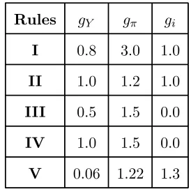
Rules gY gπ gi
I 0.8 3.0 1.0
II 1.0 1.2 1.0
III 0.5 1.5 0.0
IV 1.0 1.5 0.0
[image:8.595.225.362.295.434.2]V 0.06 1.22 1.3
Table 1: The Five Taylor (1999a) Rules
Rules III and IV are simple Taylor rules where the interest rate responds only to
real output and the inflation rate. Rule III is the original Taylor (1993) rule. Rule IV is
suggested by Henderson and McKibbin (1993) and supported by Ball (1997) and Williams
(1999) who argue that the interest rate should respond more aggressively to changes in
output. Rules, I, II and V, generalise the Taylor rule to include the lagged interest
rate. These are called “interest rate smoothing” rules since the interest rate responds
only gradually to changes in output and inflation and the interest rate is only partially
adjusted. Rule II is a simple modification of the Taylor rule with a weight on the lagged
interest rate equal to that on output. Rule I has a greater weight on inflation relative to
output than rule II. Rule V is proposed by Rotemberg and Woodford (1999) and unlike I
rate. They propose this rule following a welfare analysis that finds significant welfare
improvements by allowing the interest rate to respond to lagged values of itself.9
3
The Model
The model is a variation of the sticky-price general equilibrium structure which has,
following the approach developed by Obstfeld and Rogoff (1995, 1998), been often used
in the recent open economy macroeconomics literature.10
The model consists of two countries, a small home country and a large foreign country,
inhabited by a continuum of infinitely lived individual agents who are consumer/producers.
Agents consume a group of differentiated, perishable goods of total measure unity. These
goods are indexed by z on the unit interval. Home country agents produce fraction n
goods and foreign agents produce1−ngoods.11 Each individual agent uses labour effort
to produce a single good and is the monopoly supplier of that good. Prices are assumed
to be sticky in that some agents cannot immediately respond to economic disturbances by
changing prices within the period under consideration. Instead, these agents respond to
disturbances by meeting market demand at pre-set prices. The specific form of sluggish
price adjustment considered here is that described by Calvo (1983), which assumes that
agents change their prices after time intervals of random length such that an agent is
allowed to change the price of his/her good with probability(1−γ).
The world economy is assumed to be disturbed by a range of stochastic shocks
includ-ing labour supply shocks and government expenditure shocks originatinclud-ing in both countries.
The home and foreign monetary authorities are assumed to be following a policy which
consists of an interest rate rule of the form described in the previous section. Most of
9It is important to emphasise that none of thefive policy rules is intended to be fully optimal within
the model described below. The purpose of the papers in the Taylor (1999a) volume is to investigate the
robustness of thesefive rules across a range of different specifications, as is the objective of this paper. 10See Lane (2001) for a survey of this literature.
11nwill be taken to be small except when considering cooperation between two equal-sized countries,
the analysis focuses on the choice of monetary policy rule for the home economy when
the home economy is small relative to the foreign economy. The welfare performance
of each of the five rules is considered for the home economy under: i. different degrees
of openness of the home country; ii. for different foreign monetary policies; and iii. for
different sources of shocks hitting the home and foreign economies.
The detailed structure of the home country is described below. The foreign country
has an identical structure. Where appropriate, foreign real variables and foreign currency
prices are denoted with an asterisk.
All agents in the home economy have utility functions of the same form. The utility
of agenth is given by
Ut(h) =Et " ∞
X
s=t
βs−t
µ
C1−ρ s (h)
1−ρ +χlog
Ms(h)
Ps −
Ks
µ y
µ s (h)
¶#
(1)
where χ is a positive constant, C is a consumption index defined across all home and
foreign goods,M denotes end-of-period nominal money holdings,P is the consumer price
index,y(h) is the output of goodh andE is the expectations operator. K is a stochastic
shock to labour supply preferences which evolves as follows
logKt=ζKlogKt−1+εK,t (2)
where εK is symmetrically distributed over the interval [− , ] with E[εK] = 0 and
V ar[εK] = σ2K. An increase in K represents an increase in the marginal disutility of
labour and implies a fall in labour supply.
The consumption index C for home agents is defined as
C =h[1−(1−n)ν]1θ C θ−1
θ
H + [(1−n)ν] 1
θ C θ−1
θ
F i θ
θ−1
(3)
whereCH andCF are indices of home and foreign produced goods defined as follows
CH = "µ
1
n
¶1
φ Z n
0
cH(i)
φ−1
φ di
# φ
φ−1
, CF = "µ
1 1−n
¶1
φZ 1
n
cF (j)
φ−1
φ dj
# φ
φ−1
(4)
where φ > 1, cH(i) is consumption of home good i and cF (j) is consumption of foreign
goods. The parameter ν is a measure of openness, ν = 0 is equivalent to a completely
closed economy and ν = 1 to a completely open economy. An alternative interpretation
for this parameter is that it determines the degree of home bias. Given that one of the
purposes of the current paper is to evaluate the relative performances of thefive rules in
an open economy model, as opposed to the closed economy models of the Taylor (1999a)
volume, using a measure of openness will enable a comparison of the closed (ν = 0) and
the open (ν = 1) economy versions of this model with the closed economy models in
Taylor (1999a).
The aggregate consumer price index for home agents is
P =£[1−(1−n)ν]PH1−θ+ [(1−n)ν]PF1−θ¤
1
1−θ (5)
wherePH andPF are the price indices for home and foreign goods respectively defined as
PH =
∙
1
n
Z n
0
pH(i)
1−φ
di
¸ 1
1−φ
, PF =
∙
1 1−n
Z 1
n
pF (j)
1−φ
dj
¸ 1
1−φ
(6)
The law of one price is assumed to hold. This implies pH(i) = Sp∗H(i) and pF(j) =
Sp∗
F (j) for all i and j where an asterisk indicates a price measured in foreign currency
andS is the exchange rate (defined as the domestic price of foreign currency). However,
note that purchasing power parity does not hold in terms of aggregate consumer price
indices, due to the presence of home bias.
It is assumed that internationalfinancial trade is restricted to a risk free bond
denom-inated in the currency of the foreign country.12 Agent h’s budget constraint is
Bt(h)/St+Mt(h) = (1 +i∗t−1)ϕtBt−1(h)/St+Mt−1(h) +pH,t(h)yt(h)
−PtCt(h)−Tt+Rt(h) (7)
12In much of the recent open economy literature it is standard to assume that internationalfinancial
markets allow complete consumption risking. However, the modelling of a complete markets structure is
problematic in an asymmetric world (such as a small open economy of the type considered here). Any
asymmetry implies an asymmetry in the prices of state-contingent assets. Thus, a full analysis of a
complete markets structure requires explicit modelling of asset prices. This complication can be avoided,
and thus the model can be considerably simplified, by assuming that international financial trade is
whereB(h)is bond holdings, M(h) is money holdings and T is a lump-sum government transfer.
As is standard in much of the literature, individual agents are assumed to have access to
a market for state-contingent assets which allows them to insure against the idiosyncratic
income shocks implied by the Calvo pricing structure.13 The pay-offto agenth’s portfolio
of state-contingent assets is given byR(h).
In order to remove the unit root which arises when international financial trade is
restricted to non-contingent bonds, bond holdings are subject to a cost which is related
to the aggregate stock of bonds held. The holding cost is represented by the multiplicative
term ϕt in the budget constraint, where
ϕt= 1/(1 +δBt−1) (8)
andB is the aggregate holding of bonds by the home population.
Home agents can also hold wealth in the form of a home nominal bond which is not
internationally traded but which can be a substitute for the foreign bond amongst home
agents. The rate of return on the home nominal bond will be linked to the rate of return on
the foreign bond by the generalised uncovered interest rate parity relationship as follows
(1 +it) = (1 +i∗t)ϕt
1
St
EhSt+1C−
ρ t+1 Pt+1
i
EhC−
ρ t+1 Pt+1
i (9)
The home country’s government purchases a basket of home goods of per capita
amount Gt, prints money and makes lump sum transfers, Tt. The government budget
constraint is
Mt−Mt−1+Tt−PHGt = 0 (10)
Changes in the money supply are assumed to enter and leave the economy via changes in
lump-sum transfers.
13There is a separate market for state-contingent assets in each country and there is no international
Government purchases are subject to stochastic shocks such thatG evolves as follows
logGt=ζGlogGt−1 +εG,t (11)
where εG is symmetrically distributed over the interval [− , ] with E[εG] = 0 and
V ar[εG] = σ2G. An increase in G will mean an increase in government purchases of
the home country and will be treated as a positive real demand shock.
The intertemporal dimension of home agents’ consumption choices gives rise to the
familiar consumption Euler equation
Ct−ρ=β(1 +it)PtEt
∙
Ct−+1ρ Pt+1
¸
(12)
A similar condition holds for foreign agents.
Individual home demands for representative home good, h, and foreign good, f, are
cH(h) =CH µ
pH(h)
PH ¶−φ
, cF (f) =CF µ
pF (f)
PF ¶−φ
(13)
where
CH = [1−(1−n)ν]C µ
PH
P
¶−θ
, CF = [(1−n)ν]C µ
PF
P
¶−θ
(14)
Foreign demands for home and foreign goods have an identical structure to the home
demands. Individual foreign demand for representative home good,h, and foreign good,
f, are given by
c∗H(h) =CH∗
µ
p∗ H(h)
P∗ H
¶−φ
, c∗F (f) =CF∗
µ
p∗ F (f)
P∗ F
¶−φ
(15)
where
CH∗ =nνC∗ µ
PH∗
P∗ ¶−θ
, CF∗ = (1−nν)C∗ µ
PF∗
P∗ ¶−θ
(16)
The total demand for home goods isY =nCH+ (1−n)CH∗ +nG and the total demand
for foreign goods isY∗ =nCF + (1−n)CF∗ + (1−n)G∗.14
Prices are assumed to be set in the currency of the producer and to be sticky in that
some agents cannot immediately respond to economic disturbances by changing prices
14In line with Benigno (2001), it is assumed that the government of the home country only makes
within the period under consideration. Instead, these agents respond to disturbances by
meeting market demand at pre-set prices. The specific form of sluggish price adjustment
considered here is that described by Calvo (1983), which assumes that agents change
their prices after time intervals of random length. In other words, the specific time period
between price changes is a random variable. The probability that a given agent changes
its price in any particular period is taken to be a constant, (1−γ). Accordingly the
probability that a given agent will leave his/her price at the previous pre-determined
level is γ. Given the law of large numbers, the proportion of agents leaving their price
levels unchanged isγ, and the proportion(1−γ)reset their prices at a new optimal level.
All agents who set their price at timet choose the same price, denotedpH,t for the home
country. Thefirst-order condition for the choice of prices implies the following
Et
( ∞
X
s=t
(βγ)s−t
∙
(φ−1)pH,tyt,s
CsρPs −
φKsy µ t,s
¸)
= 0 (17)
whereyt,s = (1/n)Ys(pH,t/PH,s)−φis the period-s output of a home agent whose price was
last set in period t. It is possible to rewrite the expression for aggregate home producer
prices as follows
PH,t = " ∞
X
s=0
(1−γ)γsp1H,t−φ−s
# 1
1−φ
(18)
As described above, individual agents are assumed to have access to insurance markets
which allow them to insure against the idiosyncratic income shocks implied by the Calvo
pricing structure. In section 6, two alternative variants of the model are considered, one
with backward-looking price setting and the other with local currency pricing.
The foreign economy, except for the fact that it is a large economy (given nis small),
has an identical structure to the home economy. The foreign country is assumed to be
subject to stochastic shocks to its labour supply such thatK∗
t evolves as follows
logKt∗ =ζK∗logKt∗−1+εK∗,t (19)
where εK∗ is symmetrically distributed over the interval [− , ] with E[εK∗] = 0 and
the following form
logG∗t =ζG∗logG∗t−1+εG∗,t (20)
where εG∗ is symmetrically distributed over the interval [− , ] with E[εG∗] = 0 and
V ar[εG∗] =σ2G∗.
The main focus of attention in this paper is on the choice of monetary rule for the
small home economy. The objective is to compare the set of interest rules in Table 1.
Thus, the model is solved and a measure of welfare is derived for each of the five rules
listed in Table 1.
It is also necessary to specify the behaviour of the foreign monetary authority. The
foreign monetary authority is assumed to adopt an interest rate rule of the same general
form as the home authority, thus
ˆı∗t =gY∗Yˆt∗+gπ∗πˆ∗t +gi∗ˆı∗t−1 (21)
The values of the feedback coefficients in this policy rule will obviously affect the
behav-iour of foreign country variables and this, in turn, may have implications for the welfare
performance of the alternative monetary rules for the home economy. In the analysis
below, it is assumed that the foreign country policy rule is restricted to the set of rules
in Table 1 and the welfare comparison between home-country policy rules is conducted
separately for each of the five possible foreign monetary rules.
4
Model Solution
It is not possible to derive an exact solution to the model described above. The model
is therefore approximated around a non-stochastic equilibrium (defined as the solution
which results when K = K∗ = G = G∗ = 1 andσ2
K = σ2K∗ = σ2G = σ2G∗ = 0). For any
variableX defineXˆ = log¡X/X¯¢whereX¯ is the value of variableXin the non-stochastic
equilibrium. Xˆ is therefore the log-deviation of X from its value in the non-stochastic
Aggregate (per capita) home welfare in period 0is defined as
Ω= 1
nE0
∞ X s=0 βs ½Z n 0 µ
C1−ρ s (h)
1−ρ − Ks
µ y
µ s (h)
¶
dh
¾
(22)
where, for simplicity, the utility of real balances is excluded.
A second-order approximation ofΩ can be written as follows
¡
Ω−Ω¯¢= ¯C1−ρE0
∞ X s=0 βτ ½ ˆ
Cs+
1
2(1−ρ) ˆC
2
s
−φ−φ 1
∙
ˆ
Ys+
1
2µ( ˆYs+ 1
µKˆs) 2+1
2φ(1 +φ(µ−1))Πs
¸¾
+O¡ 3¢ (23)
where
Πs=
∞ X
i=0
(1−γ)γi³pˆH,s−i−PˆH,s ´2
(24)
whereO( 3) contains terms of order higher than two in the variables of the model.15
Note that the second-order approximation of aggregate utility depends on the first
and second moments of consumption, output and prices. In order to analyse aggregate
utility, it is necessary to derive second-order accurate solutions for the first moments of
the variables of the model. These solutions are obtained numerically using the technique
described in Sutherland (2002). The next section reports numerical solutions to the above
model (under a variety of specifications) which allow a comparison to be made between
thefive rules. The numerical solutions are obtained using the following benchmark set of
parameter values: The discount factorβ = 0.99, the elasticity of substitution for
individ-ual goods φ= 7.66, the elasticity of substitution between home and foreign goods θ= 4
16, the work effort preference parameter µ= 1.47, the elasticity of intertemporal
substi-15All log-deviations from the non-stochastic equilibrium are of the same order as the shocks, which (by
assumption) are of maximum size . When presenting an equation which is approximated up to order
two it is therefore possible to gather all terms of order higher than two in a single term denotedO¡ 3¢.
16The empirical literature on the elasticity of substitution between home and foreign goods does not
provide any clear guidance on an appropriate value for this parameter. Obstfeld and Rogoff(2000), in their brief survey of some of the literature, quote estimates ranging between 1.2 and 21.4 for individual
goods. Estimates for the average elasticity across all traded goods lie between 5 and 6 (see Hummels
(2001)). The real business cycle literature typically uses a much smaller value forθ, for instance Chari,
tution ρ= 1, bond holding costs δ= 0.001. The values forβ, φ, µ and ρ are taken from
Rotemberg and Woodford (1999). The value for δ (i.e. the parameter determining the
costs of bond holdings) is based on the calibration used by Benigno (2001). The
parame-terζi, which determines the persistence of the shocks, is set at 0.95 andσi= 0.007 for all
four sources of shocksi=K, K∗, G, G∗. Productivity shocks are assumed to be correlated
across countries with a correlation coefficient of 0.25. The government spending shocks
are similarly correlated. The size of the small open economyn, is set at0.001.
5
Comparison of Policy Rules: Small Country Case
The main objective of this paper is to use the above described open economy model to
compare the performance of the set of five Taylor (1999a) rules listed in Table 1. In
doing so, several variations of home and foreign monetary policy are analysed. In all the
cases considered, the home and foreign monetary authorities are assumed to be following
a policy which consists of an interest rate rule of the form described above. The analysis
focuses on the choice of monetary policy rule for the home economy when the home
economy is small relative to the foreign economy. The welfare performance of each of the
five rules is considered for the home economy: i. under different degrees of openness of
the home country;ii.for different foreign monetary policies ; andiii.for different sources
of shocks. Initially, a benchmark case is considered where the set offive rules is compared
when the foreign country sets its monetary policy according to the simple Taylor rule,
rule III. The effects of different foreign monetary policies are considered in section 5.2. In
the benchmark case, there is a mixture of domestic and foreign stochastic labour supply
and government expenditure shocks hitting the two countries simultaneously. Section 5.3
repeats the welfare comparison between policy rules in four separate cases where only one
of the sources of shocks is present in each case. In Section 5.4. the effects of parameter
5.1
Benchmark Results
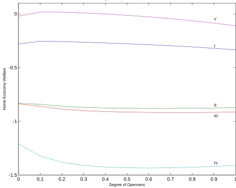
Figure 1 shows the welfare values under each of thefive rules for all degrees of economic
openness, from ν = 0, which is equivalent to a completely closed economy to ν = 1,
which is equivalent to a completely open economy.17 Figure 1 shows that the interest rule
which delivers the highest welfare for all degrees of openness is rule V, the Rotemberg
and Woodford (1999) rule. The next best rule, in terms of welfare, is rule I. Rules II and
III, (which produce very similar welfare values) produce lower welfare levels than rules
V and I, and rule IV performs worst of all in terms of welfare. Figure 1 shows that this
welfare ranking is unchanging in the degree of openness of the home economy. The welfare
performance of each rule does not seem to vary significantly with the degree of openness.
INSERT FIGURE 1 ABOUT HERE
Note that, when ν = 0, the home economy is completely closed, the results may be
compared with the results from closed economy models (Rotemberg and Woodford (1999),
Taylor (1999a, 1999b)). Figure 1 shows that, in the benchmark case, the welfare ranking
of these rules in a closed economy matches the welfare ranking in the open economy.
Thus, the differences in the transmission mechanism of monetary policy which arise in
the open economy case appear not to affect the welfare ranking of these five rules.
Some of the underlying intuition for the welfare results and other aspects of the
perfor-mance of these rules may be understood from considering the impact of the different rules
on the volatilities of the main macro variables. Table 2 reports the standard deviations
(SD) of real output, consumption, the interest rate, the inflation rate and the exchange
rate for each policy rule for three different levels of openness of the home economy. The
standard deviations of output, the inflation rate and the interest rate are relevant since
they indicate how different rules affect the trade-off between output-inflation variability
and the trade-offbetween inflation and interest rate variability.
INSERT TABLE 2 ABOUT HERE
17The numerical welfare values reported in Figure 1 and all subsequent tables are measured in units
First we compare the original Taylor rule, rule III, with rule IV which has a higher
feedback coefficient on real output. Table 2 shows that the standard deviation of real
out-put is lower and that of inflation is higher under rule IV than under rule III. This indicates
that raising gY represents a movement along the ‘output-inflation trade-off curve’.
Fig-ures 2 and 3 plot the variability of output, inflation and the interest rate for all rules, the
circles on the figure indicate each rule when the economy is closed (ν = 0), the triangles
with the number of the rule followed by the letter O indicate each rule when the economy
is open(ν = 1). Figure 2 is similar to Taylor’s policy frontier in the sense that rules that
have smaller standard deviations of output tend to have larger standard deviations of
inflation and vice versa. Figure 2 shows that moving from rule III to IV, the standard
deviation of output falls and the standard deviation of inflation rises.
INSERT FIGURES 2 AND 3 ABOUT HERE
As evident from Table 2, a higher response coefficient on real output gY, also leads
to an increase in the variability of consumption and of the interest rate compared to rule
III. There is greater interest rate variability because the higher feedback coefficient on
output induces the interest rate to respond more actively to stabilise output. Movements
in the variance of consumption is linked to the variance in the interest rate through the
consumption Euler equation, (equation (12)). Figure 3 shows that moving from rule III
to IV leads to higher variability in both the interest rate and the inflation rate so that
rule III dominates rule IV.
Now consider rules I, II and V in Table 2. Rule I has greater feedback on all variables,
Rule II has a larger feedback on output relative to inflation and rule V places a very small
weight on output relative to inflation. In comparing rule II with rule V, we are analysing
the effects of having a higher weight on output relative to inflation and vice versa. Table
2 and Figure 2 show that these rules also imply movements along the ‘output-inflation
trade-offcurve’. A higher feedback from output implies lower output variability attained
at the expense of higher volatility in inflation.
rate term. This implies some degree of interest rate smoothing which in turn, implies that
any change in the interest rate has some persistence. Given the forward-looking nature of
the model, expectations of a persistent move in the interest rate will imply that any given
change in the interest rate has a more powerful effect on variables in the current period.
Thus, the interest rate movements needed to achieve a given degree of macroeconomic
stabilisation will be smaller when there is a lagged interest rate term in the rule. This
explains why the interest rate variance is lower under rule V, for instance, (where the
feedback coefficient on the lagged interest rate is the highest of all the rules). Since the
variance of consumption follows movements in the variance of the interest rate, this also
implies that the variance of consumption is lower under rule V than the other rules.
This leads to the question of whether there is a trade-offbetween interest rate volatility
and inflation volatility. Taylor (1999b) argues that although the variability of real output
and inflation may be reduced by highly aggressive rules, such rules cause the variability
of the interest rate to increase considerably. However the results here contradict this
conclusion and Figure 3 shows that rules I and V, both highly aggressive rules, give lower
interest rate variances than rules III and IV. In fact, rules that do include it−1 lead to
lower interest rate variability than equivalent rules that do not.18
Notice that the impact of the different rules on the standard deviations reported in
Table 2, and the trade-offs discussed above, is relatively unaffected by the degree of
openness of the home economy. This can be seen in Figures 2 and 3, when the circles
(indicating the standard deviations under each rule when the home economy is closed)
are compared with the triangles (indicating the standard deviations under each rule when
the home economy is open).
18This is also in contrast to Taylor’s (1999b) finding that the variance of the interest rate is higher
in rules which react to it−1. However, Taylor (1999b) recognises that these rules perform poorly and
lead to high interest rate variability mostly in models without rational expectations. As explained above,
lagged interest-rate rules depend on agents’ forward looking behaviour for their success. Given that the
model used here includes rational expectations, it is found that all lagged interest rate rules lead to lower
The impact of the different rules on the volatilities reported above also help understand
the welfare comparison. Aggregate welfare depends negatively on the volatility of inflation
and the volatility of consumption. Thus, rules which reduce the volatility of inflation and
consumption, such as rules I and V, yield the best welfare outcome. While aggregate
welfare also depends on the volatility of output, it is the volatility of output relative to
the labour supply shock,K, which matters for welfare, not the volatility of output itself.
Hence, rules which reduce the volatility of output (such as rules III and IV) result in lower
welfare than those rules which stabilise inflation (such as rules I and V).
The analysis of the benchmark model demonstrates the superiority of rule V compared
to the other Taylor volume rules. Subsequent sections will consider a number of important
variations of the benchmark model and will show that rule V continues to outperform the
other rules. Before proceeding with that analysis, it is useful to consider rule V in more
detail and investigate the welfare implications of small variations in the coefficients of
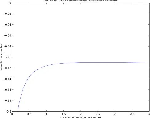
rule V in the benchmark model. Figures 4, 5 and 6 plot the welfare levels when each of
the feedback coefficientsgY, gπ andgi are varied around their benchmark values, namely
gY = 0.06, gπ = 1.22 and gi = 1.3. Figure 4 shows that if the feedback coefficient on
output is reduced to approximately zero (while holdinggπ = 1.22and gi = 1.3), there is
scope for some welfare gain, but this gain is trivial in comparison to the welfare difference
between rule V and the other rules. Figure 5 shows that there is also some scope for
increasing welfare by increasinggπ while holding gY=0.06 and gi=1.3. Within the values
forgπ plotted, welfare does not reach a maximum, however, it is clear that welfare is very
flat and welfare gains are again quite trivial compared to the welfare difference across the
five rules. Figure 6 plots welfare Ωagainstgi, (holding gY=0.06 and gπ=1.22) and shows
that a similar story holds for variations in gi. Figures 4, 5 and 6 show that the welfare
generated by rule V appears to be close to the maximum that can be achieved with a rule
of this form for the benchmark model.
INSERT FIGURES 4, 5 AND 6 ABOUT HERE
discussed and show that the welfare ranking is robust across all the variations considered.
5.2
The Impact of the Foreign Country’s Monetary Policy
The above results have shown that rule V, the Rotemberg and Woodford (1999) rule,
leads to the highest welfare level in this open economy model when the foreign country is
assumed to be following a monetary policy based on the simple Taylor rule, rule III. The
question that is now asked, is how would the performance of the five rules change (if at
all), if the large foreign country followed a rule other than rule III? Table 3 presents the
welfare values for the home country for the five cases where the foreign country follows
in turn each of thefive rules. Thus the welfare value given in rowi, columnj in Table 3
is the welfare level for the home economy when the home country follows rule j and the
foreign country follows rulei. Table 3 panel A gives the welfare results whenν = 0.5.and
panel B shows the results with ν = 1. Table 3A shows that the best policy rule for the
home country is always rule V irrespective of the rule followed by the foreign country.
The next best rule is rule I for the home country. The rule leading to the lowest welfare is
rule IV. The same pattern can be seen in the case when the home economy is completely
open, as shown in Table 3B. Thus, the welfare ranking of rules for the home economy
found in the benchmark case appears to be robust across different foreign policy rules.
INSERT TABLE 3 ABOUT HERE
5.3
Di
ff
erent Sources of Shocks
It has long been recognised that the welfare performance of monetary regimes depends
on the source of stochastic shocks hitting the economy. In the benchmark case described
above, there is a mixture of four different shocks, home and foreign real supply and
demand shocks. In order to see whether the welfare ranking identified in the benchmark
case is affected by the balance of shocks, the individual effects of each of the stochastic
real shocks are now considered separately.
of the home economy) when home labour supply shocks are theonly source of stochastic
shocks hitting the two economies have been obtained.19 These results show that, similar
to the benchmark case above, rule V generates the highest welfare, followed by rules I, II,
III and IV and that, as in the benchmark case, the degree of openness does not affect the
welfare ranking of the rules. The same exercise has been carried out whenonly stochastic
real demand shocks originating from the home country hit the two economies. As with
the case with home supply shocks, results show that the comparative welfare ranking of
the rules show a similar pattern to the benchmark case. It is again rule V that yields the
highest welfare levels, followed by rules I, II, III and IV following. Again, the degree of
openness appears to make little difference to the results obtained.20
Simulation results showing the home welfare levels for each of the five rules are also
obtained for the case when foreign labour supply shocks are theonly source of stochastic
shocks hitting the two economies. In the case where the shocks hitting the two economies
originateonly from the foreign country, it is important to note that the specific monetary
policy rule adopted by the foreign country may have implications for the relative
perfor-mance of the rules adopted by the home country. For this reason, the relative welfare
comparison of thefive home policy rules is carried out in turn for each of thefive possible
rules followed by the foreign economy. Welfare results for the case where ν = 0.5 show
that the rule which delivers the highest home welfare is rule I when the foreign country
follows rules II, III and IV.21 Results show that when the home economy is completely
open(ν = 1), it is rule V which outperforms the other rules in terms of welfare. The next
best rule is I, followed by rules II, III and IV. Thus, in general, the welfare ranking of rules
19These simulations are carried out assuming that the foreign country’s monetary policy is based on
following rule III. Note that when the shocks hitting the two countries originate solely from the home
economy, the specific foreign monetary policy rule adopted is irrelevant for the relative comparisons of
the performance of each of rules adopted by the home country (because in the absence of foreign shocks
all variables in the foreign economy do not vary in any case). 20These results are not reported but are available upon request.
21These are the only cases so far analysed where rule V is not the best rule. However, in these cases
for the home economy found in the benchmark case appears to be robust across different
foreign policy rules even when the supply shocks hitting the two economies originateonly
from the foreign economy. This exercise is repeated for the case of foreign demand shocks.
Results show that the comparative welfare ranking of the rules show a similar pattern to
the benchmark case. It is again rule V that delivers the highest welfare levels, with rules
I, III and II next.22 Rule IV again ranks the lowest in terms of home welfare. The degree
of openness appears to make little difference to the general pattern of results.23
5.4
Parameter Variations
Before concluding this section,we briefly consider the extent to which the benchmark
results are sensitive to variations in the parameters of the model. Five parameters are
likely to be important, namely, θ, ρ, φ, µ and ζj. The parameter θ, the elasticity of
substitution between home and foreign goods is likely to be important because θ is a
main determinant of the strength of the expenditure switching effect and it is known
that the expenditure switching effect can play a significant role in the welfare comparison
between rules. We consider two alternative values forθ, 0.8 and 6. The effects of increasing
ρ,which determines the elasticity of intertemporal substitution, to 6 are considered. The
parameterφdetermines the price elasticity of demand for individual goods, (see equations
(13) and (15)). The effects of setting φ to 4 and 12 are considered. The effects of setting
µ to 6 is considered which implies a significantly lower elasticity of labour supply than
the benchmark value. Finally, we look at the implications of a higher value forζi which
determines the persistence of stochastic shocks. The effects of increasing the degree of
persistence of shocks to ζi = 0.99 are analysed. Results varying these five parameters
(when there is a mixture of four different shocks, home and foreign real supply and
demand shocks, as in the benchmark case) indicate that the benchmark results are robust
to all the parameter variations carried out. Rule V continues to deliver the highest welfare
22For a degree of opennessν= 0.5,the ranking of rules II and III switch places, though the difference in welfare levels is quite small.
levels under all three degrees of openness of the home economy.24
6
Alternative Pricing Structures
This section considers two alternative assumptions regarding price-setting and tests the
robustness of the welfare ranking of the five rules under each alternative assumption.
6.1
Backward-Looking Prices
The Calvo (1983) pricing structure has been subject to criticism because it implies that
the inflation rate can adjust very rapidly to shocks. There is in fact extensive empirical
evidence suggesting that there is significant inertia in the inflation rate. One way to
model sluggish inflation is to allow for some degree of backward-looking behaviour in
price setting. It is therefore useful to analyse the robustness of the benchmark welfare
results when the benchmark framework is modified to allow some prices to be set in a
backward-looking manner. In the benchmark model above, the forward-looking nature of
price setting is evident in thefirst order condition for price setting given in equation (17).
In this section, the model is modified by assuming that producers set prices as a weighted
average of a forward-looking component, pfH,t, and a backward-looking component, pb
H,t,
such that the new price set in periodt is
pH,t=αpfH,t+ (1−α)p b H,t
where α is the weight given to the forward looking component. The forward looking
component is determined from the first-order condition (17) and the backward looking
component is determined by the following rule of thumb
pbH,t =PH,t−1+ξ(PH,t−1−PH,t−2)
where 0 < ξ < 1. Thus the backward looking component is determined by the average
level of producer prices observed in the previous period, updated by a fraction of the
observed producer price inflation rate.
Figure 7 shows the welfare values under each of thefive rules for different values of α,
fromα= 0, where producers are entirely backward-looking, toα= 1,where producers are
entirely forward-looking. Figure 7 shows that as α is reduced (i.e. as producers become
more backward looking) the welfare performance of the five rules become very similar.
Nevertheless, the interest rate rule which delivers the highest welfare is again rule V,
except for values ofα <0.1. Figure 8 shows the welfare values under each of thefive rules
for different values of ξ, where ξ measures the degree of indexation in backward-looking
pricing. Figure 8 again shows that rule V yields the highest welfare.25
INSERT FIGURES 7 AND 8 ABOUT HERE
6.2
Exchange Rate Pass-through
The benchmark model is based on the assumption that prices are set in the currency of
the producer, i.e. producer currency pricing (PCP). However, Bergin (2004)finds strong
empirical support for the alternative price setting structure, that of local currency pricing
(LCP), where prices are set in the currency of the buyer. PCP implies full pass-through
from exchange rate changes to export prices while LCP implies incomplete pass-through.
Given the empirical support for LCP, it is important to consider the impact of
in-complete exchange rate pass-through on the welfare performance of the policy rules using
the above model. Incomplete exchange rate pass-through is introduced in the model by
allowing each producer to set two prices, one for sales to home consumers, and another
for sales to foreign consumers. Each price is assumed to be subject to separate Calvo
(1983) style price setting processes. Export prices (i.e. prices for homes sales to foreign
consumers and foreign sales to home consumers) are assumed to be subject to a fixed
degree of indexation to the nominal exchange rate, denoted η. Thus, η = 0implies zero
pass-through from exchange rate changes to export prices, and η = 1 implies full pass
25In Figure 7ξis set equal to 1 and in Figure 8αis set equal to 0.5. In both figures ν = 1, which is
through.26 Figure 9 shows the welfare values for each of the five rules for different values
ofη. These results are based onν = 1. Figure 9 shows that the interest rule which delivers
the highest welfare for all degrees of pass-through is again rule V with the ranking of the
rules exactly the same as in the benchmark analysis.
INSERT FIGURE 9 ABOUT HERE
7
The Two-Country Case
The analysis of the choice of the five policy rules now turns to the case where the size
of the home and foreign countries are equal, i.e. n = 0.5. In the small open economy
case, by definition, the choice of policy rule for the home economy has no impact on
macroeconomic outcomes or welfare in the foreign economy, so the choice of policy rule
by the foreign country is independent from the choice of home policy rule. However, when
the home economy is large it becomes necessary to analyse jointly the choice of policy
rules in both countries. This is best achieved by thinking of the choice of policy rule as
being the equilibrium of a policy game. This section will analyse both the coordinated
and the non-coordinated choice of policy rules in a game of this type.
INSERT TABLES 4 AND 5 ABOUT HERE
Table 4 shows the pay-offmatrices for the policy game where the pay-offs are the levels
of aggregate welfare yielded by combinations of home and foreign policy rules. Table 4
panel A shows the welfare levels for the home economy for thefive cases where the foreign
country follows each of thefive rules and panel B presents the welfare levels for the foreign
country for thefive cases where the home country follows each of thefive rules. (Thus the
welfare value given in rowi, columnjin Table 4A is the welfare level for the home economy
when the home country follows rulej and the foreign country follows rule iand similarly
in Table 4 panel B.) The results in Table 4A and B are obtained under the assumption
that the degree of openness of the both countries is set atν = 0.5. Table 5 panels A and
B present the results under the assumption that both countries are completely open.
The home welfare levels reported in Table 4A, shows that irrespective of the policy
rule followed by the foreign country, the home country obtains the highest welfare by
following rule V. For the foreign country, Table 4B shows that rule V again yields the
highest welfare irrespective of the policy rule followed by the home country. In the case
where the two economies are completely open (shown in Table 5A) it is seen that this
pattern is repeated and that rule V continues to yield higher welfare levels for each country
regardless of policy rule followed by the other.
The results presented in Tables 4 and 5 show that, irrespective of the degree of
open-ness, rule V is a dominant strategy for both countries. Rule V is therefore both a Nash
equilibrium and the coordinated equilibrium in a game over the choice of policy rules.
That is, whether the two countries act cooperatively or not, the policy rule which
de-livers the highest welfare for each country is rule V. As such, these results are in exact
accordance with the results of the benchmark case of the small economy analysis.27
8
Open Economy Interest Rate Rules
The above sections have extended the closed economy analysis of thefive Taylor (1999a)
rules to an open economy setting and also investigated the robustness of these rules in a
variety of different configurations. However, open economy issues such as the behaviour of
exchange rates and the importance of the exchange rate as a key transmission mechanism
of monetary policy, especially in transmitting the effects foreign shocks, are central to
27Tables 4 and 5 are based on the case where shocks are the benchmark mixture of home and foreign
real supply and real demand disturbances. The pay-offmatrices (not reported) which correspond to the four cases where only individual sources of shocks are present show that in all cases rule V is always
a dominant strategy and is thus always both a coordinated and non-coordinated equilibrium choice for
monetary policy. It is often suggested in policy circles that monetary policy should be
used, to some extent, to mitigatefluctuations in the nominal exchange rate. Indeed, there
is some empirical evidence that central banks do follow policy rules which include a role
for the exchange rate. For instance, Lubik and Schorfheide (2005) and Bergin (2004)find
evidence that the Federal Reserve, the Bank of Canada and the Bank of England follow
policy rules which include a positive feedback term in the exchange rate. This indicates
that policy has been, to some extent, directed towards stabilising the nominal exchange
rate for these countries. In the context of this paper, this suggests that it is interesting
to analyse the welfare implications of adding an exchange rate term into the interest
rate rule. A number of theoretical papers have also considered the role of the exchange
rate in policy rules. The conclusions reached in this line of literature are rather mixed.
Ball (1999) suggests that including the exchange rate brings a relatively large benefit,
while others such as Adolfson (2002), Batini, Harrison and Millard (2003) and Leitemo
and Söderstrom (2005) report only minor improvements from including the exchange rate
in the rule. Taylor (2001) also concludes that including a direct feedback term on the
exchange rate only brings a minor benefit.
INSERT TABLE 6 ABOUT HERE
One key feature of this existing line of the literature is that it is based on ad hoc
measures of welfare rather than the utility-based welfare measure used in this paper. It
is therefore valuable to re-examine this issue using the current model. Table 6 shows a
number of variants of rule V which include the rate of change of the nominal exchange
rate with coefficients ranging from -0.1 to -0.5. It is apparent that there is some welfare
improvement obtained by including such a term. However, note that the size of the welfare
gain is very small and it appears that these welfare gains are possible only if the coefficient
on the rate of change of the exchange rate is negative. This implies that stabilising the
exchange rate is welfare decreasing rather than welfare increasing.
Another issue which has received some attention in the open economy literature on
analysis is based on using the consumer price index (CPI). Since one of the fundamental
welfare costs of inflation volatility in models, such as the one analysed here, is its impact
on relative price distortions across producers, it is often argued that monetary policy in
an open economy should aim to stabilise producer price inflation.28 It is therefore useful
to consider an alternative form of rule V which includes PPI inflation rather than CPI
inflation. The welfare results of this rule is shown in the final column of Table 6. It is
apparent that the CPI form of rule V delivers marginally higher welfare than the PPI
version, but the welfare difference between the two versions of the rule is minimal.
9
Conclusions
This paper uses an open-economy model to compare the relative welfare performances
of the set of five interest rate rules of the Taylor (1999) volume. This is done using a
stochastic dynamic model which is more general than those that have been widely used
in the recent open-economy literature (in the sense that welfare results are obtained for
unrestricted parameter values). A rule with a lagged interest rate term, high feedback
on inflation and low feedback on output is found to perform well in terms of stabilising
inflation and attaining the highest welfare for a small open economy. This result is shown
to be robust across different degrees of openness of the home economy, for alternative
foreign monetary rules, different sources of home and foreign shocks, a set of key parameter
variations and for alternative pricing structures. A two-country version of the model
analysing the same set of rules shows that the rule that performs best in the
small-country analysis also emerges as both the Nash and cooperative equilibria in the
two-country case. While this paper focused on a comparison between a fixed set of policy
rules, a brief analysis of more general rules, with open economy elements, was considered.
This limited analysis showed that in this framework no significant welfare improvements
were to be obtained.
References
[1] Adolfson, M. (2002) “Incomplete Exchange Rate Pass-through and Simple Monetary
Policy Rules” Working Paper No. 136, Sveriges Riksbank.
[2] Ball, L. (1997) “Efficient Rules for Monetary Policy.” NBER WP No. 5952.
[3] Ball, L. (1999) “Policy Rules for Open Economies.” In J. B. Taylor (ed.) Monetary
Policy Rules,University of Chicago Press, Chicago, 127-144.
[4] Batini, N. and Haldane, A. (1999) “Forward-Looking Rules for Monetary Policy” in
J. B. Taylor (ed.)Monetary Policy Rules, University of Chicago Press,
Chicago,157-192.
[5] Batini, N., Harrison, R. and Millard, S. P. (2003) “Monetary Policy Rules for an
Open Economy.” Journal of Economic Dynamics and Control, 27, 2059-94.
[6] Benigno, P. (2001) “Price Stability with Imperfect Financial Integration.” CEPR
Discussion Paper No. 2854.
[7] Benigno, G. and Benigno, P. (2003) “Price Stability in Open Economies” Review of
Economics Studies, 70, 743-764.
[8] Benigno, P. and Woodford, M. (2004) “Inflation Stabilization and Welfare: The Case
of a Distorted Steady State” NBER Working Paper No. 10838
[9] Bergin, P. (2003) “Putting the ‘New Open Economy Macroeconomics’ to a Test”
Journal of International Economics, 60, 3-34.
[10] Bergin, P. (2004) “How Well can the New Open Economy Macroeconomics Explain
the Exchange Rate and the Current Account” NBER WP No. 10356
[11] Bergin, P., Shin, H and Tchakarov, I. (2005) “Does Exchange Rate Variability Matter
for Welfare? A Quantitative Investigation of Stabilization Policies” University of
[12] Calvo, G. A. (1983) “Staggered Prices in a Utility-Maximising Framework.”Journal
of Monetary Economics,12, 383-98.
[13] Chari, V. V. , Kehoe, P. J. and McGrattan, E. R. (2002) “Can Sticky Price Models
Generate Volatile and Persistent Real Exchange Rates?”Review of Economic Studies,
69, 533-64.
[14] Clarida, R., Gali, J. and Gertler, M. (1999) “The Science of Monetary Policy: A New
Keynesian Perspective.” Journal of Economic Literature 37, 1661-1707.
[15] Clarida, R., Gali J. and Gertler, M. (2002) “A Simple Framework for International
Monetary Policy Analysis” Journal of Monetary Economics, 49, 879-904.
[16] Corsetti, G. and Pesenti, P. (2004) “International Dimensions of Optimal Monetary
Policy.” Journal of Monetary Economics, 52, 281-305.
[17] Devereux, M. B. (2004) “Should the Exchange Rate be a Shock Absorber?” Journal
of International Economics, 62, 359-378.
[18] Devereux, M. B. and Engel, C. (2003) “Monetary Policy in an Open Economy
Re-visited: Price Setting and Exchange Rate Flexibility” Review of Economic Studies,
70,765-783.
[19] Gali, J. and Monacelli, T. (2005) “Monetary Policy and Exchange Rate Volatility in
a Small Open Economy”Review of Economics Studies, 72,
[20] Henderson, D. and McKibbin, W. (1993), “An Assessment of Some Basic Monetary
Policy Regime Pairs.” in R. Bryant (ed.)Evaluating Policy Regimes: New Research
in Macroeconomics, Brookings Press, Washington.
[21] Hummels, D. (2001) “Towards a Geography of Trade Costs.” Purdue University,
unpublished manuscript.
[22] Juillard, M., Karam, P,. Laxton, D. and Pesento, P. (2005) “Welfare-Based Monetary
[23] King, R. G. and Wolman, A. L. (1999) “What Should the Monetary Authority do
When Prices are Sticky?” in J. B. Taylor (ed.)Monetary Policy Rules, University of
Chicago Press, Chicago, 349-98.
[24] Kirsanova, T., Leith, C. and Wren-Lewis, S. (2006) “Should Central Banks Target
Consumer Prices or the Exchange Rate?”Economic Journal, 116, F208-F231.
[25] Kollmann, R. (2002) “Monetary Policy Rules in the Open Economy: Effects on
Welfare and Business Cycles.”Journal of Monetary Economics, 49, 989-1015.
[26] Lane, P. (2001) “The New Open Economy Macroeconomics: A Survey.” Journal of
International Economics, 54, 235-66.
[27] Leitemo, K. and Söderstrom, U. (2005) “Simple Monetary Policy Rules and Exchange
Rate Uncertainty”Journal of International Money and Finance, 24, 481-507.
[28] Lubik, T. A. and Schorfheide, F. (2005) “Do Central Banks Respond to Exchange
Rate Movements? A Structural Investigation” Journal of Monetary Economics,
forthcoming.
[29] McCallum, B. and Nelson, E. (1999) “Performance of Operational Policy Rules in an
Estimated Semi-classical Structural Model.” in J. B. Taylor (ed.) Monetary Policy
Rules,University of Chicago Press, Chicago, 15-45.
[30] Obstfeld, M. and Rogoff, K. (1995) “Exchange Rate Dynamics Redux.” Journal of
Political Economy, 103, 624-60.
[31] Obstfeld, M. and Rogoff, K. (1998) “Risk and Exchange Rates.” NBER Working
Paper No. 6694.
[32] Obstfeld, M. and Rogoff, K. (2000) “The Six Major Puzzles in International
Macro-economics: Is There a Common Cause?”NBER Macroeconomics Annual, 15, 339-90.
[33] Obstfeld, M. and Rogoff, K. (2002) “Global Implications of Self-Oriented National