End to end audiovisual speech recognition

arXiv:1802.06424v2 [cs.CV] 22 Feb 2018

END-TO-END AUDIOVISUAL SPEECH RECOGNITION

Stavros Petridis

_{, Themos Stafylakis}

_{, Pingchuan Ma}

_{, Feipeng Cai}

Georgios Tzimiropoulos

_{, Maja Pantic}

1

_{Dept. of Computing, Imperial College London, UK}

_{Computer Vision Laboratory, University of Nottingham, UK}

stavros.petridis04@imperial.ac.uk, themos.stafylakis@nottingham.ac.uk

ABSTRACT

Several end-to-end deep learning approaches have been re-cently presented which extract either audio or visual features from the input images or audio signals and perform speech recognition. However, research on end-to-end audiovisual models is very limited. In this work, we present an end-to-end audiovisual model based on residual networks and Bidi-rectional Gated Recurrent Units (BGRUs). To the best of our knowledge, this is the first audiovisual fusion model which simultaneously learns to extract features directly from the im-age pixels and audio waveforms and performs within-context word recognition on a large publicly available dataset (LRW). The model consists of two streams, one for each modality, which extract features directly from mouth regions and raw waveforms. The temporal dynamics in each stream/modality are modeled by a 2-layer BGRU and the fusion of multiple streams/modalities takes place via another 2-layer BGRU. A slight improvement in the classification rate over an end-to-end audio-only and MFCC-based model is reported in clean audio conditions and low levels of noise. In presence of high levels of noise, the end-to-end audiovisual model significantly outperforms both audio-only models.

Index Terms— Audiovisual Speech Recognition,

Resid-ual Networks, End-to-End Training, BGRUs, AudiovisResid-ual Fusion

1. INTRODUCTION

Traditional audiovisual fusion systems consist of two stages, feature extraction from the image and audio signals and com-bination of the features for joint classification [1, 2, 3]. Re-cently, several deep learning approaches for audiovisual fu-sion have been presented which aim to replace the feature ex-traction stage with deep bottleneck architectures. Usually a transform, like principal component analysis (PCA), is first applied to the mouth region of interest (ROI) and spectro-grams or concatenated Mel-Frequency Cepstral Coefficients

ACCEPTED TO ICASSP 2018

(MFCCs) and a deep autoencoder is trained to extract bottle-neck features [4, 5, 6, 7, 8, 9]. Then these features are fed to a classifier like a support vector machine or a Hidden Markov Model.

Few works have been presented very recently which follow an end-to-end approach for visual speech recogni-tion. The main approaches followed can be divided into two groups. In the first one, fully connected layers are used to ex-tract features and LSTM layers model the temporal dynamics of the sequence [10, 11]. In the second group, a 3D convolu-tional layer is used followed either by standard convoluconvolu-tional layers [12] or residual networks (ResNet) [13] combined with LSTMs or GRUs. End-to-end approaches have also been successfully used for speech emotion recognition using 1D CNNs and LSTMs [14].

However, work on end-to-end audiovisual speech recog-nition has been very limited. To the best of our knowledge, there are only two works which perform end-to-end training for audiovisual speech recognition [15, 16]. In the former, an attention mechanism is applied to both the mouth ROIs and MFCCs and the model is trained end-to-end. However, the system does not use the raw audio signal or spectrogram but relies on MFCC features. In the latter, fully connected lay-ers together with LSTMs are used in order to extract features directly from raw images and spectrograms and perform clas-sification on the OuluVS database [17].

emo-(a) (b)

Fig. 1. Example of mouth ROI extraction.

tion recognition. The main differences of our work are the following: 1) we use a ResNet for the audio stream instead of a rather shallow 2-layer CNN, 2) we do not use a pre-trained ResNet for the visual stream but we train a ResNet from scratch, 3) we use BGRUs in each stream which help modeling the temporal dynamics of each modality instead of using just one BLSM layer at the top and 4) we use a training procedure which allows for efficient end-to-end training of the entire network.

We perform classification of 500 words from the LRW database achieving state-of-the-art performance for audiovi-sual fusion. The proposed system results in an absolute in-crease of 0.3% in classification accuracy over the end-to-end audio-only model and an MFCC-based system. The end-to-end audiovisual fusion model also significantly outperforms (up to 14.1% absolute improvement) the audio-only models under high levels of noise.

2. LRW DATABASE

For the purposes of this study we use the Lip Reading in the Wild (LRW) database [19] which is the largest publicly avail-able lipreading dataset in the wild. The database consists of short segments (1.16 seconds) from BBC programs, mainly news and talk shows. It is a very challenging set since it con-tains more than 1000 speakers and large variation in head pose and illumination. The number of words, 500, is also much higher than existing lipreading databases used for word recog-nition, which typically contain 10 to 50 words [20, 21, 17].

Another characteristic of the database is the presence of several words which are visually similar. For example, there are words which are present in their singular and plural forms or simply different forms of the same word, e.g., America and American. We should also emphasise that words appear in the middle of an utterance and there may be co-articulation of the lips from preceding and subsequent words.

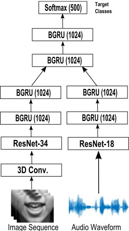
3. END-TO-END AUDIOVISUAL SPEECH RECOGNITION

The proposed deep learning system for audiovisual fusion is shown in Fig. 2. It consists of two streams which extract

3D Conv.

Softmax (500) TargetClasses

ResNet-18

Image Sequence Audio Waveform

ResNet-34 BGRU (1024)

BGRU (1024)

BGRU (1024)

BGRU (1024) BGRU (1024)

BGRU (1024)

Fig. 2. Overview of the end-to-end audiovisual speech recog-nition system. Two streams are used for feature extraction directly from the raw images and audio waveforms. The tem-poral dynamics are modelled by BGRUs in each stream. The top two BGRUs fuse the information of the audio and visual streams and jointly model their temporal dynamics.

features directly from the raw input images and the audio waveforms, respectively. Each stream consists of two parts: a residual network (ResNet) [22] which learns to automat-ically extract features from the raw image and waveform, respectively and a 2-layer BGRU which models the temporal dynamics of the features in each stream. Finally, 2 BGRU layers on top of the two streams are used in order to fuse the information of the audio and visual streams.

3.1. Visual Stream

The visual stream is similar to [13] and consists of a spa-tiotemporal convolution followed by a 34-layer ResNet and a 2-layer BGRU. A spatiotemporal convolutional layer is ca-pable of capturing the short-term dynamics of the mouth re-gion and is proven to be advantageous, even when recurrent networks are deployed for back-end [12]. It consists of a convolutional layer with 64 3D kernels of 5 by 7 by 7 size (time/width/height), followed by batch normalization and rec-tified linear units.

ImageNet or CIFAR). Finally, the output of ResNet-34 is fed to a 2-layer BGRU which consists of 1024 cells in each layer.

3.2. Audio Stream

The audio stream consists of an 18-layer ResNet followed by two BGRU layers. There is no need to use a spatiotemporal convolution front-end in this case as the audio waveform is an 1D signal. We use the standard architecture for the ResNet-18 with the main difference being that we use 1D instead of 2D kernels which are used for image data. A temporal kernel of 5ms with a stride of 0.25ms is used in the first convolu-tional layer in order to extract fine-scale spectral information. The output of the ResNet is divided into 29 frames/windows using average pooling in order to ensure the same frame rate as the video is used. These audio frames are then fed to the following ResNet layers which consist of the default kernels of size 3 by 1 so deeper layers extract long-term speech char-acteristics. The output of the ResNet-18 is fed to a 2-layer BGRU which consists of 1024 cells in each layer (using the same architecture as in [13]).

3.3. Classification Layers

The BGRU outputs of each stream are concatenated and fed to another 2-layer BGRU in order to fuse the information from the audio and visual streams and jointly model their temporal dynamics. The output layer is a softmax layer which provides a label to each frame. The sequence is labeled based on the highest average probability.

4. EXPERIMENTAL SETUP

4.1. Preprocessing

Video:The first step is the extraction of the mouth region of interest (ROI). Since the mouth ROIs are already centered, a fixed bounding box of 96 by 96 is used for all videos as shown in Fig. 1. Finally, the frames are transformed to grayscale and are normalized with respect to the overall mean and variance. Audio: Each audio segment is z-normalised, i.e., has zero mean and standard deviation one to account for variations in different levels of loudness between the speakers.

4.2. Evaluation Protocol

The video segments are already partitioned into training, val-idation and test sets. There are between 800 and 1000 se-quences for each word in the training set and 50 sese-quences in the validation and test sets, respectively. In total there are 488766, 25000, and 25000 examples in the training, valida-tion and test sets, respectively.

4.3. Training

Training is divided into 2 phases: first the audio/visual streams are trained independently and then the audiovisual network is trained end-to-end. During training data augmen-tation is performed on the video sequences of mouth ROIs. This is done by applying random cropping and horizontal flips with probability 50% to all frames of a given clip. Data augmentation is also applied to the audio sequences. During training babble noise at different levels (between -5 dB to 20 db) might be added to the original audio clip. The selection of one of the noise levels or the use of the clean audio is done using a uniform distribution.

4.3.1. Single Stream Training

Initialisation: First, each stream is trained independently. Directly training end-to-end each stream leads to suboptimal performance so we follow the same 3-step procedure as in [13]. Initially, a temporal convolutional back-end is used in-stead of the 2-layer BGRU. The combination of ResNet and temporal convolution (together with a softmax output layer) is trained until there is no improvement in the classification rate on the validation set for more than 5 epochs. Then the temporal convolutional back-end is removed and the BGRU back-end is attached. The 2-layer BGRU (again with a sotf-max output layer) is trained for 5 epochs, keeping the weights of the 3D convolution front-end and the ResNet fixed. End-to-End Training: Once the ResNet and the 2-layer BGRU in each stream have been pretrained then they are put together and the entire stream is trained end-to-end (using a softmax output layer). The Adam training algorithm [24] is used for end-to-end training with a mini-batch size of 36 se-quences and an initial learning rate of 0.0003. Early stopping with a delay of 5 epochs was also used.

4.3.2. Audiovisual Training

Initialisation:Once the single streams have been trained then they are used for initialising the corresponding streams in the multi-stream architecture. Then another 2-layer BGRU is added on top of all streams in order to fuse the single stream outputs. The top BGRU is first trained for 5 epochs (with a softmax output layer), keeping the weights of the audio and visual streams fixed.

End-to-End Training: Finally, the entire audiovisual net-work is trained jointly using Adam with a mini-batch size of 18 sequences and an initial learning rate of 0.0001. Early stopping is also applied with a delay of 5 epochs.

5. RESULTS

Table 1. Classification Rate (CR) of the Audio-only (A), Video-only (V) and audiovisual models (A + V) on the LRW database. *This is a similar end-to-end model which uses a different mouth ROI, computed based on tracked facial land-marks, in each video. In this work, we use a fixed mouth ROI for all videos.

Stream CR

A (End-to-End) 97.7 A (MFCC) 97.7 V (End-to-End) 82.0 V [13]* 83.0 V [15] 76.2 V [19] 61.1 A + V (End-to-End) 98.0

audio/audiovisual results on the LRW database we also com-pute the performance of a 2-layer BGRU network trained with MFCC features which are the standard features for acoustic speech recognition. We use 13 coefficients (and their deltas) using a 40ms window and a 10ms step. The network is trained in the same way as the BGRU networks in section 4.3 with the only difference that it was trained for longer using early stopping.

The end-to-end audio system results in a similar perfor-mance to MFCCs which is a significant result given that the input to the system is just the raw waveform. However, we should note that the effort required in order to train the end-to-end system is significantly higher than the 2-layer BGRU used with MFCCs. The end-to-end audiovisual system leads to a small improvement over the audio-only models of 0.3%. This is expected since the contribution of the visual modality is usually marginal in clean audio conditions as reported in previous works as well [1, 16].

In order to investigate the robustness to audio noise of the audiovisual fusion approach we run experiments under vary-ing noise levels. The audio signal for each sequence is cor-rupted by additive babble noise from the NOISEX database [25] so as the SNR varies from -5 dB to 20 dB.

Results for the audio, visual and audiovisual models un-der noisy conditions are shown in Fig. 3. The video-only classifier (blue solid line) is not affected by the addition of the audio noise and therefore its performance remains con-stant over all noise levels. On the other hand, as expected, the performance of the audio classifier (red dashed line) is sig-nificantly affected. Similarly, the performance of the MFCC classifier (purple solid line) is also significantly affected by noise. It is interesting to point out that although the MFCC and end-to-end audio models result in the same performance when audio is clean or under low levels of noise (10 to 20 dB), the end-to-end audio model results in much better per-formance under high levels of noise (-5 dB to 5 dB). It results

-5 0 5 10 15 20

SNR (dB)

60 65 70 75 80 85 90 95 100

CR

V A AV MFCC

Fig. 3. Classification Rate (CR) as a function of the noise level. A: End-to-End audio model. V: End-to-End visual model, AV: End-to-End audiovisual model. MFCC: A 2-layer BGRU trained with MFCCs.

in an absolute improvement of 0.9%, 3.5% and 7.5% over the MFCC classifier, at 5 dB, 0 dB and -5 dB, respectively.

The audiovisual model (yellow dotted line) is more ro-bust to audio noise than the audio-only models. It performs slightly better under low noise levels (10 dB to 20 dB) but it significantly outperforms both of them under high noise levels (-5 dB to 5 dB). In particular, it leads to an absolute improvement of 1.3%, 3.9% and 14.1% over the end-to-end audio-only model at 5 dB, 0 dB and -5 dB, respectively.

6. CONCLUSION

In this work, we present an end-to-end visual audiovisual fu-sion system which jointly learns to extract features directly from the pixels and audio waveforms and performs classifi-cation using BGRUs. Results on the largest publicly avail-able database for within-context word recognition in the wild show that the end-to-end audiovisual model slightly outper-forms a standard MFCC-based system under clean conditions and low levels of noise. It also significantly outperforms the end-to-end and MFCC-based audio models in the presence of high levels of noise. A natural next step would be to extend the system in order to be able to recognise sentences instead of isolated words. Finally, it would also be interesting to in-vestigate in future work an adaptive fusion mechanism which learns to weight each modality based on the noise levels.

7. ACKNOWLEDGEMENTS

8. REFERENCES

[1] G. Potamianos, C. Neti, G. Gravier, A. Garg, and A. W. Senior, “Recent advances in the automatic recognition of audiovisual speech,” Proceedings of the IEEE, vol. 91, no. 9, pp. 1306–1326, Sept 2003.

[2] S. Dupont and J. Luettin, “Audio-visual speech model-ing for continuous speech recognition,”IEEE Trans. on Multimedia, vol. 2, no. 3, pp. 141–151, 2000.

[3] S. Petridis and M. Pantic, “Prediction-based audiovisual fusion for classification of non-linguistic vocalisations,”

IEEE Transactions on Affective Computing, vol. 7, no. 1, pp. 45–58, 2016.

[4] J. Ngiam, A. Khosla, M. Kim, J. Nam, H. Lee, and A. Y Ng, “Multimodal deep learning,” in Proc. of ICML, 2011, pp. 689–696.

[5] D. Hu, X. Li, and X. Lu, “Temporal multimodal learn-ing in audiovisual speech recognition,” inIEEE CVPR, 2016, pp. 3574–3582.

[6] H. Ninomiya, N. Kitaoka, S. Tamura, Y. Iribe, and K. Takeda, “Integration of deep bottleneck features for audio-visual speech recognition,” inInterspeech, 2015.

[7] Y. Mroueh, E. Marcheret, and V. Goel, “Deep multi-modal learning for audio-visual speech recognition,” in

IEEE ICASSP, 2015, pp. 2130–2134.

[8] Y. Takashima, R. Aihara, T. Takiguchi, Y. Ariki, N. Mi-tani, K. Omori, and K. Nakazono, “Audio-visual speech recognition using bimodal-trained bottleneck features for a person with severe hearing loss,” Interspeech, pp. 277–281, 2016.

[9] S. Petridis and M. Pantic, “Deep complementary bottle-neck features for visual speech recognition,” inICASSP, 2016, pp. 2304–2308.

[10] S. Petridis, Z. Li, and M. Pantic, “End-to-end visual speech recognition with LSTMs,” in IEEE ICASSP, 2017, pp. 2592–2596.

[11] M. Wand, J. Koutnik, and J. Schmidhuber, “Lipreading with long short-term memory,” inIEEE ICASSP, 2016, pp. 6115–6119.

[12] Y. M. Assael, B. Shillingford, S. Whiteson, and N. de Freitas, “Lipnet: Sentence-level lipreading,”arXiv preprint arXiv:1611.01599, 2016.

[13] T. Stafylakis and G. Tzimiropoulos, “Combining resid-ual networks with LSTMs for lipreading,” in Inter-speech, 2017, vol. 9, pp. 3652–3656.

[14] G. Trigeorgis, F. Ringeval, R. Brueckner, E. Marchi, M. Nicolaou, B. Schuller, and S. Zafeiriou, “Adieu features? end-to-end speech emotion recognition us-ing a deep convolutional recurrent network,” inIEEE ICASSP, 2016, pp. 5200–5204.

[15] J. S. Chung, A. Senior, O. Vinyals, and A. Zisserman, “Lip reading sentences in the wild,”IEEE CVPR, 2017.

[16] S. Petridis, Y. Wang, Z. Li, and M. Pantic, “End-to-end audiovisual fusion with LSTMs,” inAuditory-Visual Speech Processing Conference, 2017.

[17] I. Anina, Z. Zhou, G. Zhao, and M. Pietik¨ainen, “Ouluvs2: A multi-view audiovisual database for non-rigid mouth motion analysis,” inIEEE FG, 2015, pp. 1–5.

[18] P. Tzirakis, G. Trigeorgis, M. A. Nicolaou, B. Schuller, and S. Zafeiriou, “End-to-end multimodal emotion recognition using deep neural networks,” IEEE Journal of Selected Topics in Signal Processing 2017.

[19] J. S. Chung and A. Zisserman, “Lip reading in the wild,” inACCV. Springer, 2016, pp. 87–103.

[20] M. Cooke, J. Barker, S. Cunningham, and X. Shao, “An audio-visual corpus for speech perception and automatic speech recognition,” The Journal of the Acoustical So-ciety of America, vol. 120, no. 5, pp. 2421–2424, 2006.

[21] E. Patterson, S. Gurbuz, Z. Tufekci, and J. Gowdy, “Moving-talker, speaker-independent feature study, and baseline results using the CUAVE multimodal speech corpus,” EURASIP J. Appl. Signal Process., vol. 2002, no. 1, pp. 1189–1201, Jan. 2002.

[22] K. He, X. Zhang, S. Ren, and J. Sun, “Deep residual learning for image recognition,” inIEEE CVPR, 2016, pp. 770–778.

[23] K. He, X. Zhang, S. Ren, and J. Sun, “Identity mappings in deep residual networks,” inECCV. Springer, 2016, pp. 630–645.

[24] D. Kingma and J. Ba, “Adam: A method for stochastic optimization,”arXiv preprint arXiv:1412.6980, 2014.