A method for matching crowd sourced and authoritative geospatial data

A Method for Matching Crowd-sourced and Authoritative Geospatial Data

Heshan Du, Natasha Alechina, Michael Jackson, Glen Hart University of Nottingham, UK

Abstract

A method for matching crowd-sourced and authoritative geospatial data is presented. A level of tolerance is defined as an input parameter as some difference in the geometry representation of a spatial object is to be expected. The method generates matches between spatial objects using location information and lexical information, such as names and types, and verifies consistency of matches using reasoning in qualitative spatial logic and description logic. We test the method by matching geospatial data from OpenStreetMap and the national mapping agencies of Great Britain and France. We also analyze how the level of tolerance affects the precision and recall of matching results for the same geographic area using 12 different levels of tolerance within a range of 1 to 80 meters. The generated matches show potential in helping enrich and update geospatial data.

1. Introduction

Maps, whether digital or paper-based, are a common feature of our daily life. They typically provide a two-dimensional representation of geographic features, such as roads, rivers, buildings, places, etc., in the real world (i.e. a topographic base) over which other ‘thematic’ information may be displayed such as density of population or crime statistics. The information represented provides both an indication of where on the earth’s surface an object of interest is (i.e. its geometry) and lexical information on what that geometry represents (e.g. a road and its name such as ‘High Street’). Such information represented in maps is often referred to as geospatial data and plays an essential role in many governmental, economic and social operations, such as disaster response, urban planning and tourism.

Traditionally, most national level mapping was carried-out by government agencies or specialist mapping companies, because it required the use of expensive or difficult-to-obtain survey data, plus specialist tools and later software and an associated high-level of expertise. Geospatial data which is surveyed and classified using formal quality assurance procedures, for example by a national mapping agency, is referred to be ‘authoritative’. Maps produced by the general public, who did not have access to such data sources, nor the specialist tools and software, focused more on smaller areas and on indicating where key features were in relative terms but typically could not be relied upon for precise location, completeness or consistency. This situation has been radically changed in recent years by a number of technological developments and by

which is something else. The concept of ‘crowd-sourced geospatial data’ was expressed in different ways, such as citizen science, volunteered or involuntary geospatial information, user-generated content, public participation or collaboratively contributed geographic information and neogeography, in literature from 1990 to 2014 (Goodchild 2007, Heipke 2010, Comber et al.

2014). OpenStreetMap (OSM) (OpenStreetMap 2014) is the most popular map project of crowd-sourced data. Compared to authoritative data, crowd-crowd-sourced data is usually less geometrically accurate, less formally structured and lacks the associated metadata that allows it to be used in situations where commercial, policy or life-critical use is involved (Jackson et al. 2010). However, crowd-sourced geospatial data still offers great potential as it often contains richer user-based information, can reflect real world changes (e.g. new constructions of buildings) more quickly, and has a much lower acquisition cost. It is desirable to use authoritative and crowd-sourced data to complement each other in order to provide a more complete, up-to-date, people-centric and richer picture of geospatial data. One promising application of this is to use crowd-sourced geospatial data to help national mapping agencies enrich and update authoritative data.

Governments invest large amounts of money in national mapping agencies, which act as the primary source of geospatial information in many countries. In order to provide the most up-to-date maps to customers, it is essential for national mapping agencies to upup-to-date their data

frequently and regularly. However, this is expensive in both time and money. Taking Ordnance Survey of Great Britain (OSGB) (Ordnance Survey 2014a), Great Britain’s national mapping authority, as an example, according to its agency performance monitors, one of the OSGB 2013-2014 targets is ‘some 99.6% of significant real-world features greater than six months old are represented in the database’ (Ordnance Survey 2014b). To achieve this, OSGB employs a number of different methods:

• Major construction companies are contracted to provide change intelligence concerning

where and when they will build and site plans enabling Ordnance Survey to schedule field survey in a timely fashion. This will capture a significant amount of change intelligence related to all major building sites, road construction and other large construction events.

• OSGB collects planning permissions from local authorities.

• OSGB receives change reports from individual surveyors who have observed any change in

their local areas.

• OSGB captures further changes using aerial imagery. This can be used to capture missed

major changes, such as a single house and a farm barn (that does not require a planning permission). It will also capture a lot of minor changes, such as new or removed hedgerows and paths.

• OSGB also receives change reports (e.g. letters, emails or phone calls) from the general public, but these reports only comprise a very small proportion of all the intelligence received.

becoming increasingly important as OSGB moves from being simply a map producer to one that wishes to supply much richer geographic information.

As shown by the example of OSGB, current working methods employed by national mapping agencies leave room for improvement and are faced with challenges raised by the rapid

development of crowd-sourced geospatial data. As EuroGeographics’ President, Ingrid Vanden Berghe (Geospatial PR 2014), says, ‘Europe’s National Mapping, Cadastral and Land Registry Authorities must adapt their activities to become geospatial information brokers if they are to continue to meet society’s expectations’. This indicates that national mapping agencies will collate data rather than just collect data in future, except for areas where only national mapping agencies are able to collect the data.

Figure 1: Huntingdon Primary and Nursery School represented in OSGB (stippled), OSM (solid) and their relative position

Figure 2: Victoria Shopping Centre represented in OSGB (stippled), OSM (solid) and their relative position

To use crowd-sourced data for enriching and updating authoritative data, it is essential to establish correspondence (matches) between spatial features represented in crowd-sourced and authoritative geospatial data. By using the established matches, descriptions about the

However, matching disparate geospatial data is far from straightforward. In different geospatial datasets, different terminologies or vocabularies are often used to describe spatial features. For example, the same restaurant may be classified as a Restaurant in one dataset, whilst as a Place

to Eat in another database and simply as a brand-name in others (e.g. McDonald’s). An

identically spelt word, even within a single language, can often have many different meanings. Whilst an authoritative dataset will have a defined taxonomy or ontology where a word should have a precise definition, the ‘crowd’ may not follow such rules and may use several descriptions for a common object some of which may be local vernacular terms. For example, the word

College may mean an institution within a university in one dataset, refer to a government

secondary school in another and a private language training establishment in a third. Other terms may be used inconsistently, for instance, one person may include McDonald’s within the

category restaurant whilst others may not. For the same geographic area or the same set of spatial features, different geospatial data sources will have different representative geometries. Features may be represented in one dataset, but not in the other. The scale or accuracy of the geometry capture may vary. Even where the same precision of measurement is adopted, different points may be captured to represent the boundary of a feature so that two independently captured representations of a single object will always differ in some respect. As shown in Figure 1, the position and shape of Huntingdon Primary and Nursery School are represented differently in OSGB data (stippled) and OSM data (solid). In Figure 2, the Victoria Shopping Centre is represented as several shops in OSGB, but as a whole in OSM.

In this paper, we present a generic method for matching spatial objects held in different datasets with no shared form of digital identity. A spatial object in a geospatial dataset has an ID,

location information and meaningful labels, such as names or types, and represents an object in the real world. A geometry here refers to a point, a line or a polygon, which is used to represent location information in geospatial datasets. We use both location information and lexical information to generate matches, and then check consistency of matches using reasoning in qualitative spatial logic and description logic. This idea has been implemented as a software tool called MatchMaps and its main steps have been described briefly in Du et al. (2015b), but without providing detailed algorithms for generating matches. This is what we do in this paper. To tolerate slight differences in geometric representations for the same spatial feature, the matching algorithms use a level of tolerance σ∈ R≥ 0 as input. The evaluation presented in Du et al. (2015b) is extended to show how the value of σ affects matching results. In Du et al. (2015b), the method was used to match OSM data and OSGB data. In this paper, we additionally use the method to match OSM data and data from IGN (Institut Géographique National 2014), the national mapping agency of France.

Geospatial data matching is defined as the task of identifying corresponding spatial features between different geospatial datasets. It is an essential step for data comparison, data integration or enrichment, change detection and data update. Over the last few decades, many methods (such as Walter and Fritsch 1999, Mustire and Devogele 2008, Tong et al. 2009, Safra et al. 2010, 2013, Li and Goodchild 2011, Huh et al. 2013, Tong et al. 2014) have been developed for matching authoritative geospatial data. Du (2015) provided a summary of these methods and discussed the limitations of them. None of these methods have been widely accepted and

generally applied. The methods designed for matching authoritative geospatial data are not very suitable for OpenStreetMap (OSM) data, due to the information incompleteness and inaccuracy in OSM data, as well as its informal or non-standard representations. With the development of sourced geospatial data, several attempts have been made in order to match crowd-sourced geospatial data and authoritative geospatial data in the last few years.

Anand et al. (2010) applied map matching techniques to match road networks by calculating average distance and angle. However, it is computationally expensive and limited to linear features.

Ludwig et al. (2011) implemented an automated procedure for matching street networks of Navteq and OSM in Germany. Geometries and thematic attributes are compared to generate matches. However, it is specifically designed for business and geomarketing purpose, excluding features of no business interest.

Du et al. (2011) defined the meaning of ‘same feature’ regarding positional closeness, name similarity, category similarity and neighbourhood similarity. Then the probability of two spatial features being the same is calculated using a weighted function taking all these parameters into account. This work is preliminary and leaves the task of assigning weights of parameters to users.

Du et al. (2012) defined geometry consistency and topological consistency for road networks.

Two lines are geometrically consistent with respect to a level of tolerance σ, if and only if they fall into the σ-buffer of each other. Topological consistency is checked using a description logic reasoner Pellet (Sirin et al. 2007), by comparing values of a functional data property ‘neighbour set’. A neighbour set stores all the neighbours of an edge (two edges are neighbours if they have the same node). However, checking such topological consistency is too strict, due to inaccuracy and incompleteness of OSM data.

Koukoletsos et al. (2012) proposed an automated matching method for linear data in order to assess the completeness of OSM data compared to OSGB. It consists of seven stages and uses distance, orientation and attribute (road name and type) similarity constraints to generate and refine matches. However, with the existence of topological inconsistencies in OSM data, the method is not very efficient. In addition, the method does not handle abbreviations (which exist in OSM data) well when matching attributes.

matching OSM and authoritative data are of high precision. However, the method is computationally expensive, and does not use attribute data, like road names.

Yang et al. (2014) proposed a method for matching points of interest from a crowd-sourced dataset and road networks from an authoritative dataset. It first constructs a connectivity graph by mining linear cluster patterns from points, then matches nodes in the graph to roads by probabilistic relaxation and a vector median filtering. The method assumes that linear patterns exist among the points. The performance of the method mainly depends on the clustering result of points.

Fan et al. (2014) introduced a method for matching building footprints (polygons), in order to assess the quality of OSM data. Their similarity measure is defined by the percentage of overlap area, using 30% as the threshold for matching footprints. By the experimental result of the study area in Munich, the method achieves very high precision and recall, both over 99%. However, the similarity measure will fail, for example, when the same building is represented as two disjoint polygons in OSM data and authoritative data.

Most of the methods discussed above are designed for matching roads or other linear features (except Fan et al. 2014) and do not support the verification of matches (except Du et al. 2012). In this paper, we present a new method for matching crowd-sourced and authoritative geospatial data. It uses both location information and lexical information such as names and types to generate matches, and verifies consistency of matches using reasoning in description logic and qualitative spatial logic. The method was used to match buildings and places (polygonal features) represented in several real world datasets. In experiments, it achieved high precision and recall, as well as reduced human effort.

3. Method

In this section, we present a method for matching spatial features in disparate geospatial datasets. The method consists of two main steps: matching geometries and matching spatial objects. The geometry matching is based on the concepts of ‘possibly partOf’ and ‘possibly sameAs’. Section 3.1 explains algorithms used for matching geometries. Section 3.2 describes a procedure

following which spatial objects are matched using geometry matches and lexical information. The method has a wider application than matching authoritative and crowd-sourced data and could be applied wherever it is necessary to match two geospatial datasets of vector data.

3.1 Matching Geometries

Figure 3: The three hatched red circles are buffered part of (BPT) the solid blue circle (left); Buffered Equal or BEQ (right)

Definition 3.1: According to ISO19107 (ISOTechnical Committee 211 2003), the buffer of a geometry g is a geometry which contains exactly all the points within σdistance from g, where σ ∈ R≥ 0. This is formalized as:

buffer(g,σ) = {p | ∃ q ∈ g : d(p,q) ∈ [0,σ]}.

buffer(g, σ) and g are in the same reference system and dimension.

Definition 3.2: Let σ∈ R≥ 0 denote a level of tolerance. For two geometries g1 and g2, BPT(g1,g2) (g1 is buffered part of g2), iff g1 ⊆ buffer(g2,σ); BEQ(g1, g2) (g1and g2are buffered equal), iff

BPT(g1, g2) and BPT(g2, g1).

If BEQ and BPT are defined by an appropriate level of tolerance σ∈ R≥ 0, then for geometries X

and Y, if BEQ(X, Y), then X and Y possibly represent the same real world location, otherwise, they represent different locations. Similarly, if BPT(X, Y), then X represents a location which is possibly part of what Y refers to. The geometry matching method presented in this section is based on this rationale, and takes a level of tolerance σ∈ R≥ 0 as input for matching two sets of geometries. This σdenotes the maximal difference between geometric representations of the same spatial features from input datasets. The value of σcan be established empirically by looking at two datasets side by side and matching geometries of features (e.g. landmarks) which are known to be the same.

The geometry matching method consists of two main algorithms, Algorithm 2 and Algorithm 3, which generate BPT and BEQ matches respectively, by calculating and comparing the minimal σs (Definition 3.3).

Figure 4: minσ(X, Y) = d1 and minσ(Y, X) = d2

The measure minσ is not symmetric. As shown in Figure 4, X is a red circle and Y is a blue circle. Then the minimal level of tolerancewith respect to X and Y is d1, whilst the minimal level of tolerancewith respect to Y and X is d2. Though defined independently, the minimal level of tolerance was proved to be a measure equivalent to the directed Hausdorff distance, which is a generic measure for geometries (Du, 2015).

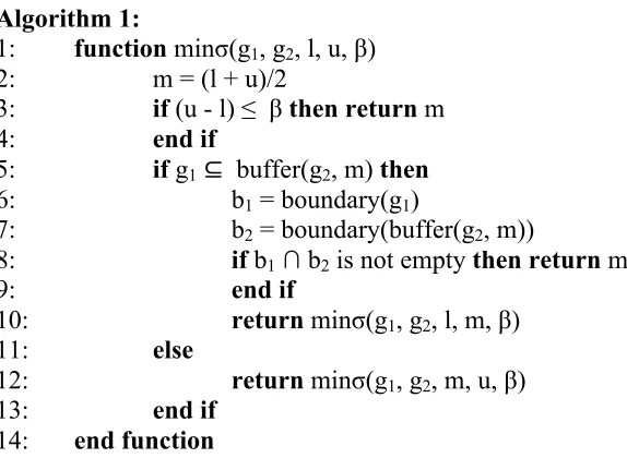
Algorithm 1 provides a way to calculate the minimal σwith respect to geometries g1 and g2 approximately. The input real numbers l and u denote a lower bound and an upper bound of σ∈

R≥ 0 respectively: σ ∈ [l, u], l ∈ R≥ 0 , u ∈ R≥ 0 . The number β∈ R≥ 0 denotes the accuracy level,

such that the absolute difference between the calculated value and the actual value of σ is no larger than β. Algorithm 1 does a ‘binary search’ between the lower bound l and the upper bound u of σ. It terminates and returns a calculated value m for the minimal σ, if m is accurate enough (Line 3) or a boundary case is reached, where g1 ⊆ buffer(g2, m) and the boundaries of g1 and buffer(g2, m) are connected (Line 8, g1 and buffer(g2, m) are equal or g1 is a tangential proper part of buffer(g2, m)).

Algorithm 1:

1: function minσ(g1, g2, l, u, β) 2: m = (l + u)/2

3: if (u - l) ≤ β then return m

4: end if

5: if g1 ⊆ buffer(g2, m) then

6: b1 = boundary(g1)

7: b2 = boundary(buffer(g2, m))

8: if b1 ∩ b2 is not empty then return m

9: end if

10: return minσ(g1, g2, l, m, β)

11: else

12: return minσ(g1, g2, m, u, β)

13: end if

Algorithm 2 takes two sets of geometries G1, G2 and a level of tolerance σ∈ R≥ 0 as input. For each geometry g1 in G1, it calculates the best candidate h in G2, and add BPT(g1, h) to the set of output matches MG1→G2, if such an h exists. The minimal σis used as the criterion to select the

best candidates (Definition 3.4).

Definition 3.4: For a geometry g, a set of geometries S, a level of tolerance σ∈ R≥ 0, the geometry h1 ∈ S is the best candidate for g, iff minσ(g, h1) < σ, and for any h ∈ S, minσ(g,h) ≥ minσ(g,h1).

Algorithm 2:

1: function bpt-match(G1, G2, σ)

2: MG1→ G2 = {}

3: for g1 ∈ G1 do

4: h = null

5: for g2 ∈ G2 do

6: if minσ(g1, g2) < σ then

7: σ = minσ(g1, g2)

8: h = g2

9: end if

10: end for

11: if h != null then

12: add BPT(g1, h) to MG1→G2

13: end if

14: end for

15: return MG1→G2

16: end function

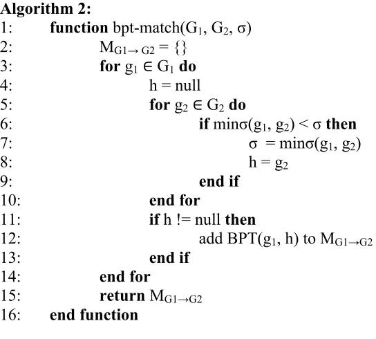
Algorithm 3 calculates BEQ matches using BPT matches generated by Algorithm 2. For every geometry g2 ∈ G2, Algorithm 3 matches it to a geometry Gs which is a union of geometries in G1, such that g2 and Gs are buffered equal, if such a Gs exists. This is done as follows. For every geometry g2 ∈ G2, we firstly obtain a set S containing every g1 ∈ G1 such that BPT(g1, g2) is in MG1→G2 (Lines 2-5). Since each geometry g ∈ S is buffered part of g2, their union Gs is buffered part of g2. If g2 is also buffered part of Gs (Line 7), then g2 and Gs are buffered equal. Generating

BEQ matches between g2 and Gs directly may have some side effects or noise, especially when

Gs consists of several disconnected parts (Gs is multiple, Line 8). Three examples are shown in Figure 5, where in each, the blue solid geometry is buffered equal to the union of several red stippled geometries. The extra red stippled geometries actually do not have any correspondences. The best candidates found for them using Algorithm 2 are the blue solid geometries, but the matches are wrong since the level of tolerance allowedis too large. Algorithm 4 is designed to refine Gs in such case, by calculating and comparing the minimal σs (Definition 3.3).

Algorithm 3:

1: function beq-match(G1, G2, σ) 2: MG1→G2=bpt-match(G1, G2, σ)

4: for g2 ∈ G2 do

5: S = {g1 ∈  G1 | BPT(g1, g2) ∈ MG1→G2}

6: Gs = ⋃g∈S g

7: if BPT(g2, Gs) then

8: if Gs is multiple then

9: Gs = refine(Gs, g2, σ)

10: end if

11: add BEQ(g2, Gs) to Mbeq

12: end if

13: end for

14: return Mbeq 15: end function

Figure 5: BEQ matches with ‘noise’

Algorithm 4:

1: function refine(Gs, g2, σ) 2: s = minσ(g2, Gs)

3: for g ∈ Gs.getGeometries() do

4: if g2 contains g then continue

5: end if

6: remain = Gs ∖ g

7: if BPT(g2, remain) does not hold then continue

8: end if

9: sr = minσ(g2, remain) // sr ≥ s

10: if s = sr then return refine(remain, g2, σ)

11: end if

12: t = minσ(Gs, g2)

13: tr = minσ(remain, g2)

17: return Gs 18: end function

Algorithm 4 takes two geometries Gs, g2 as input, where Gs is multiple and g2 is not. Gs and g2 are buffered equal with respect to the level of tolerance σ. Algorithm 4 refines Gs to a subset of it, and maintains the buffered equal relation as an invariant during the refining process. This is done as follows. For every geometry g contained in Gs, if g is not fully covered by g2, then we obtain

remain, which is Gs without g (Line 6). To maintain the invariant, we check whether

BEQ(remain, g2) holds. Since BPT(Gs, g2) and remain ⊂  Cs, BPT(remain, g2) already holds. Thus, we only need to check whether g2 is buffered part of remain. If yes, the next steps in the for-loop are followed. We calculate the minimal σ(Definition 3.3) with respect to g2 and Gs (Line 2), g2 and remain (Line 9) as s and sr respectively. By Definition 3.3, Definition 3.1 and

remain ⊂ Gs, sr ≥s. If s and sr are equal, thenwe can remove g from Gs without changing the required buffer size(Line 10). After applying this, the extra red geometries in Figure 5 (left and middle) are removed, as shown in Figure 6 (left and middle) respectively. However, the extra geometries in Figure 5 (right) cannot be removed, because the boundary of the blue geometry is close to the red geometries outside, the existence of which makes the required buffer size smaller. For such case, we calculate the minimal σwith respect to Gs and g2 (Line 12), remain

and g2 (Line 13), as t and tr respectively. If (s + t) ≥(sr + tr), we can remove g from Gs without making the sum of required buffer sizes larger (Line 14). Applying this removes the extra

geometries in Figure 5 (right), as shown in Figure 6 (right). Algorithm 4 recursively removes one part from Cs and returns the remaining parts, until no parts can be removed.

Figure 6: Refined BEQ matches

After applying Algorithm 4, Algorithm 3 generates and adds refined BEQ matches to its output mapping Mbeq.

3.2 Matching Spatial Objects

In this section, we describe a method for matching spatial objects, making use of BEQ matches generated by Algorithm 3 and lexical descriptions (names and types) of spatial objects. A

sameAs match between spatial objects a and b states that a and b represent the same real world object. This is denoted as sameAs(a, b). A partOf match from a spatial object a to a spatial object

partOf (a, b). The output of the object matching method is a set of sameAs and partOf matches between spatial objects. The method does not directly use BPT matches generated by Algorithm 2, mainly because spatial objects and their parts may not have any similar lexical information.

As a function, objects(g) maps every geometry g to a set of spatial objects, where the geometry of each object gi ⊆ g. For any pair of geometries g1 and g2 which are BEQ-matched, we match

objects(g1) and objects(g2) based on the similarity of lexical information (names and types represented by strings).

The similarity measure for lexical information is described as follows. For strings s1 and s2,

similar(s1, s2) is true, if s1, s2 are equal, one contains the other, one is an abbreviation of the other, or their Levenshtein edit distance is smaller than length(s1)/2 or length(s2)/2. For any spatial object o, let names(o) denote its set of names, types(o) denote its set of types. For any pair of spatial objects o1,o2, similarNames(o1, o2) is true, if there exist n1 ∈ names(o1) and n2 ∈

names(o2) such that similar(n1, n2). Otherwise, similarNames(o1, o2) is false. similarTypes(o1, o2) is defined in the same way as defining similarNames(o1, o2). For the type similarity, using string comparison is not sufficient, and more sophisticated similarity measures should be used to recognize different words expressing the same type, for example, house, dwelling and

residential. Currently, such information is only hard-coded for houses. For spatial object o,

house(o) is true, if the type of o is house, dwelling or residential. Otherwise, house(o) is false.

Figure 7: All are houses except one.

For any pair of geometries g1 and g2 which are BEQ-matched by Algorithm 3, objects(g1) and

objects(g2) are matched as follows:

Case 1: If |objects(gi)| = 0, i ∈ {1, 2}, then there are no objects to match.

Case 2: If |objects(gi)| = 0, |objects(gj)| > 0, i != j, then objects in objects(gj) do not have any corresponding objects.

Case 3: If |objects(gi)|= 1, i ∈{1, 2}, oi ∈objects(gi), similarNames(o1,o2) is true, or names(o1) is empty, or names(o2) is empty, then we generate a sameAs match between o1 and o2.

Case 4: If |objects(gi)|= 1, |objects(gj)| > 1, i != j, then:

a) If there exists exactly one object oj ∈ objects(gj), such that for oi ∈objects(gi),

Case 5: If |objects(gi)|> 1, i ∈{1, 2}, then:

a) If there exists at most one object o in objects(gi) such that house(o) is false, and for any other object oi in objects(gi), house(oi) is true, then we create an abstract object Oi corresponding to the aggregation of all objects in objects(gi). For every object oj∈

objects(gj), i != j, we generate a partOf match from oj to Oi.

As shown in Figure 7, there is only one spatial object (yellow) which is not a house, and all others are houses. Matching every spatial object is not interesting but requires much more effort than creating and matching an abstract object for them.

b) If no abstract object is created, then we match objects by their names first and then by their types.

i. For objects o1 ∈ objects(g1), o2 ∈  objects(g2), if similarNames(o1, o2), then we generate all possible matches: a sameAs match between o1 and o2, partOf matches from o1 to o2 and from o2 to o1.

ii. For ‘not-matched’ objects o1 ∈  objects(g1), o2∈objects(g2), if at least one of

names(o1) and names(o2) is empty, and at least one of similarTypes(o1, o2) and (house(o1) ∧house(o2)) is true, then we generate a sameAs match between o1 and

o2, partOf matches from o1 to o2and from o2 to o1.

Then we use our new qualitative spatial logic LBPT (Du and Alechina 2014a, b) to verify consistency of the generated matches with respect to location information. LBPT was designed for reasoning about geometries represented in different geospatial datasets, in particular crowd-sourced datasets. The relations between geometries considered in the logic are: BPT, Near and Far. By Definition 3.2, BEQ is definable by BPT. The relations Near and Far are also defined using a level of tolerance σ. LBPT formalizes different cases where a contradiction can be detected by LBPT reasoning. For any pair of spatial objects a and b, we assumed that if sameAs(a, b) is true, then the geometry of a and the geometry of b are BEQ; if partOf (a, b) is true, then the geometry of a is BPT the

geometry of b, where BEQ and BPT are defined using an appropriate level of tolerance σ. A contradiction exists, for example, if spatial objects a1 is sameAsa2, b1 is sameAsb2, a1 and b1 are near, but a2 and b2 are far. As an optional step, we could use description logic to verify consistency of the generated matches with respect to UNA/NPH (Unique Name Assumption/No PartOf Hierarchy) (Du et al. 2015b) after using spatial logic. For

example, an inconsistency exists, if a spatial object is stated as being sameAs two spatial objects in another dataset. This step could be skipped if UNA/NPH is violated frequently in an input dataset.

Finally, we use description logic to verify consistency of all generated matches with respect to classification information. For example, an inconsistency exists, if sameAs(o1, o2), o1 is a Bank,

4. Evaluation

In (Du et al. 2015b), we established the precision and recall of the method for matching OSM data (building layer) (OpenStreetMap 2014) and OSGB MasterMap data (Address Layer and Topology Layer) (Ordnance Survey 2014a) using a single value of σ (the level of tolerance). In

(Du et al. 2015a), we evaluated the method with respect to the amount of human effort required

for resolving contradictions detected by reasoning in spatial logic and description logic, and showed that the human effort was reduced compared to a fully manual matching process. In this section, we extend the previous evaluation in two ways. Firstly, we use several different values of σ for matching the same area represented in OSM data and OSGB MasterMap data and explain how the value of σ affects the matching results. The study area is in the city centre of Nottingham, UK. Secondly, we apply the method to match OSM data and IGN data (BD TOPO database, buildings and toponymy layers) (Institut Géographique National 2014) to show the generality of the method. The study area is a central area in Paris, France.

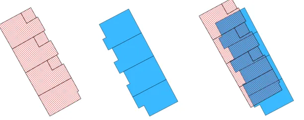
As explained already in (Du et al. 2015b), before applying the method presented in Section 3, we used standard 2D spatial tools to aggregate adjacent OSM geometries automatically so that a block of houses can be matched together. Figure 8 shows the geometric representations of the same block of houses in OSGB data (stippled) and OSM data (solid). From OSM data, we only know all of them are houses. Matching the houses one by one is time-consuming and not helpful for enriching OSGB/IGN data.

Figure 8: The geometric representations of the same block of houses in OSGB data (stippled), OSM data (solid) and their relative position.

4.1 Nottingham Case Study

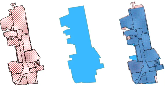
Figure 9: The geometric representations of Nottingham city centre from OSGB (left) and OSM (right)

We apply the method several times to match spatial objects in the Nottingham case using a variety of σ values. The ground truth is established in the same way as explained in (Du et al.

2015b). For each OSM spatial object, we classify it into one of the following categories by checking all the generated matches involving it: ‘Correctly Matched’ (True Positive or TP), ‘Incorrectly Matched’ (False Positive or FP), ‘Correctly Not-matched’ (True Negative or TN)

and ‘Incorrectly Not-matched’ (False Negative or FN). If a spatial object is incorrectly matched but should be matched (i.e. there exists a correct match for it), then we label it as FPsbm. Note that the size of each category is the number of OSM spatial objects in it. For example, for the Victoria Centre in OSM data, though there are hundreds of partOf matches involving it, it is only counted as one element in ‘Correctly Matched’. Precision is computed as the ratio of |TP| to |TP|

+ |FP|, and recall as the ratio of |TP| to |TP| + |FN| + |FPsbm|.

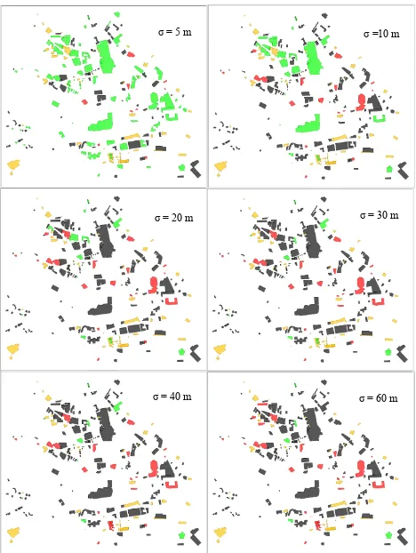
take some other values (1, 3, 5 and 15 meters) because the precision/recall changes more quickly from 0 to 10 meters and from 10 to 20 meters. For the matching results obtained by taking 5 meters, 10 meters, 20 meters, 30 meters, 40 meters and 60 meters as the level of tolerance, Figure 10 visualizes the geometries of spatial objects in different categories as maps. In (Du et al. 2015b), we estimated the appropriate level of tolerance for the Nottingham case to be 20 meters and established the precision and recall. The matching results obtained here using σ =20 meters are slightly different from those presented in (Du et al. 2015b), because the graphical user interface was modified (see Du et al. 2015a) with simpler but fewer options provided to users for retracting wrong matches. Based on the matching results obtained using different σ values

presented in Table 2, using σ = 20 meters achieves both relatively high precision and recall compared to others. This justifies that σ = 20 meters is appropriate and a good estimate. However, it is not the optimal, as the matching results obtained using σ = 30 meters are of the same precision but slightly higher recall than those obtained using σ = 20 meters. In the

Figure 10: OSM spatial objects of the Nottingham case are classified into four categories: TP (Black), FP (Red), TN (Yellow) and FN (Green).

σ = 5 m _{σ =10 m}

σ = 40 m

σ = 30 m

σ = 60 m

σ = 20 m

σ = 40 m

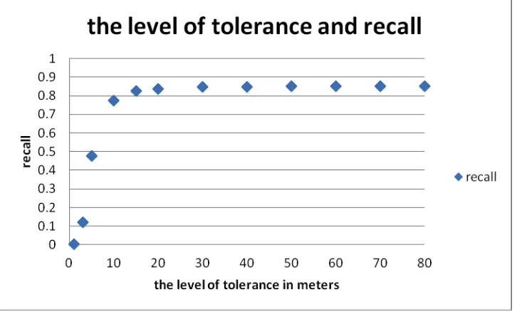
As shown in Table 2, when the level of tolerance σ is 1 meter, only 1 spatial object is correctly matched, and all others are not matched. Hence the recall is nearly 0. With the increase of the σ

value, as shown in Figure 10, more spatial objects are correctly matched. For example, in Figure 11, the Arkwright building of the Nottingham Trent University is represented as a concave geometry in OSGB data but as a convex geometry in OSM data, which can be matched using σ = 30 meters but not σ = 20 meters.

Figure 11: Nottingham Trent University’s Arkwright building represented in OSGB (stippled), OSM (solid) and their relative position

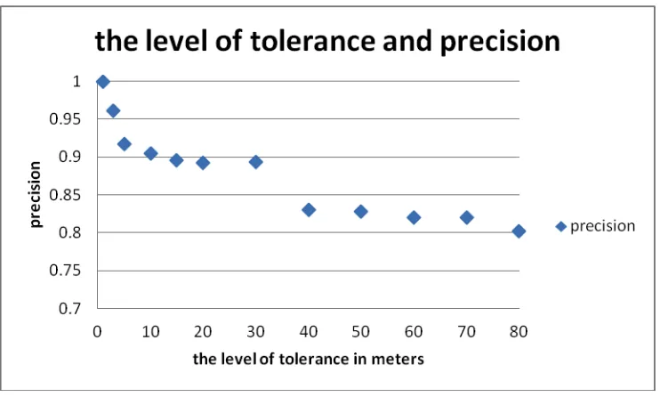
As shown in Table 2 and Figure 13, increasing the level of tolerance σ from 1 to 80 meters, the precision falls but it is always ≥ 0.8. The precision becomes lower when σ increases, mainly because a larger level of tolerance makes more spatial objects to be incorrectly stated as being

partOf some other spatial objects nearby. It is difficult to prevent such mistakes because spatial objects and their parts may not have any similar lexical information and therefore partOf

matches are generated mostly based on geometry matching. Though the generated matches will be verified using reasoning in spatial logic and description logic, not all mistakes can be

detected. For example, increasing the value of σ from 30 to 40 meters, the main concourse, ticket office, travel center and some other offices or shops within the Nottingham train station

represented in OSM are all incorrectly stated as being partOf the Xpress Catering within the Nottingham trains station represented in OSGB, as their geometries are matched. Such wrong

partOf matches are not detected by spatial logic because the objects involved are all near to each other. They are not detected by description logic because some OSM spatial objects do not have any type information and the use of description logic for verifying consistency of partOf matches (Du et al. 2015b) is limited by a small set of manually generated `partOf-disjointness’ statements (e.g. a School cannot be partOf a Pub) and does not cover the types involved in the wrong

matches. As a result, the precision drops from 0.89 to 0.83. Despite this, the precision is quite stable when σ varies from 5 to 30 meters and from 40 to 80 meters, staying around 0.9 and 0.82 respectively.

Figure 13: the level of tolerance and precision

4.2 Paris Case Study

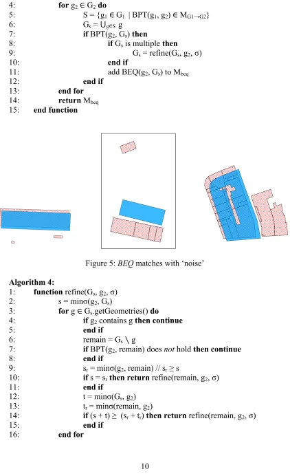
In this section, we report the use of the method for matching OSM data and IGN data (BD TOPO database, buildings and toponymy layers) (Institut Géographique National 2014). The study area is a central area in Paris, France. The data used in the Paris case was obtained in 2013 and is shown in Figure 14. Its statistics are summarized in Table 3. Differing from OSGB MasterMap data, the IGN BD TOPO database does not contain any names of premises within buildings. Therefore, the spatial objects in IGN are generated only using names of buildings. Since most of the buildings in IGN data do not have a name, the number of spatial objects in IGN data is small.

Figure 14: The geometric representations of the central area of Paris from IGN (left) and OSM (right)

We set the value of σ to be 40 meters such that the Île de la Cité island in Paris can be matched. Interestingly, the positional accuracy of OSM data has been estimated to be about 40 meters in France (Girres and Touya 2010). The ground truth is established manually in the same way as explained for the Nottingham case. The geometries of OSM spatial objects which are ‘Correctly Matched’ (True Positive or TP), ‘Incorrectly Matched’ (False Positive or FP), ‘Correctly Not-matched’ (True Negative or TN) and ‘Incorrectly Not-matched’ (False Negative or FN) are visualized in Figure 15. Their statistics are shown in Table 4. The precision and recall are both ≥

83%. Since the number of generated matches in the Paris case is small, the precision and recall are achieved by the method fully automatically. In other words, the reasoning in spatial logic and description logic does not detect any inconsistency and thus requires no human effort for

Figure 15: OSM spatial objects of the Paris case are classified into four categories: TP (Black), FP (Red), TN (Yellow) and FN (Green).

5. Application

The matches generated by the method have several practical uses. Firstly, the matches can help validate the correctness of corresponding data in input datasets. If similar records of a spatial feature exist in both input datasets which are developed independently, then the records have a higher chance of being correct. In addition, the matches facilitate information exchange and enrichment, as one dataset may contain more detailed lexical descriptions or more user-based information than the other. For example, classification descriptions of spatial features in OSM data can be more precise and more understandable by non-specialists. There are several spatial features in OSM data, such as shopping centres, hospitals and schools, which correspond to collections or aggregations of spatial features in OSGB.

the same location, and the OSM data provides more user-based information which can help enrich OSGB data.

Figure 16: The geometries of the Las Vegas Nails in OSGB data (stippled) and the New York Nails in OSM data (solid) are BEQ-matched.

Figure 17: The geometries of the Network Rail Ltd. in OSGB data (stippled) and the NEMS Platform One Medical Practice in OSM data (solid) are BEQ-matched.

Figure 18: The geometries of the Wastenot Reclamation Ltd. in OSGB data (stippled) and the Eastcroft Incinerator in OSM data (solid) are BEQ-matched.

free and can capture not only major changes but also many minor changes in buildings and roads noticed by OSM contributors, as well as changes in function or purpose. It is difficult for OSGB to capture such minor changes and functional changes using current methods. Using the OSM change intelligence seems promising but needs more advanced techniques for validating the correctness of crowd-sourced data and to be tested in practice.

6. Conclusions

In this paper, we present a generic method for matching crowd-sourced and authoritative geospatial data. It generates sameAs and partOf matches between spatial objects using both location and lexical information, and verifies consistency of matches using reasoning in qualitative spatial logic and description logic. The method is applied for matching OSM data, OSGB data and IGN data. For the Nottingham case, increasing the level of tolerance from 1 to 80 meters, the precision falls slowly and is always ≥ 0.8, the recall increases and converges at 0.85. For the Paris case, using 40 meters as the level of tolerance, a precision of 0.88 and a recall of 0.83 are achieved. Theoretically, the method presented can be used to match objects having polygonal, linear or point geometries. As future work, the generality of this method will be tested further by matching point or linear spatial features. In addition, we will use matches for

enriching and updating geospatial data, and minimize the amount of human effort required during this process.

Acknowledgements

We express thanks to Ordnance Survey of Great Britain and Institut Géographique National of France for providing the test data.

References

Anand S, Morley J, Jiang W, Du H, Jackson M J, and Hart G 2010 When Worlds Collide: Combining Ordnance Survey and Open-StreetMap data. In Proceedings ofAssociation for Geographic Information (AGI) GeoCommunity ’10 Conference

Comber A, Schade S, See L, Mooney P, and Foody G 2014 Semantic analysis of Citizen Sensing, Crowdsourcing and VGI. In Proceedings of the 17th AGILE International Conference

on Geographic Information Science ISBN: 978-90-816960-4-3

Du H 2015 Matching Disparate Geospatial Datasets and Validating Matches using Spatial

Logic. PhD thesis, School of Computer Science, University of Nottingham.

Du H and Alechina N 2014a A Logic of Part and Whole for Buffered Geometries. In

Proceedings of the 21st European Conference on Artificial Intelligence (ECAI), 997–998

Du H and Alechina N 2014b A Logic of Part and Whole for Buffered Geometries. In

Du H, Alechina N, Hart G, and Jackson M J2015a A Tool for Matching Crowd-sourced and Authoritative Geospatial Data. In Proceedings of the International Conference on Military

Communications and Information Systems (accepted, available at

http://www.cs.nott.ac.uk/~hxd/paper/A-Tool-Du-ID31.pdf)

Du H, Alechina N, Jackson M, and Hart G2013 Matching Formal and Informal Geospatial Ontologies. Lecture Notes in Geoinformation and Cartography Geographic Information Science

at the Heart of Europe. Springer, 155–171

Du H, Anand S, Alechina N, Morley J G, Hart G, Leibovici D G, Jackson M J, and Ware J M 2012 Geospatial Information Integration for Authoritative and Crowd Sourced Road Vector Data. Transactions in GIS, 16 (4), 455–476

Du H, Jiang W, Anand S, Morley J, Hart G, and Jackson M J2011 An Ontology-based Approach for Geospatial Data Integration. In Proceedings of the 25th International Cartography

Conference, CO-118

Du H, Nguyen H H, Alechina N, Logan B, Jackson M J, and Goodwin J 2015b Using Qualitative Spatial Logic for Validating Crowd-Sourced Geospatial Data. In Proceedings of the 29th AAAI Conference on Artificial Intelligence, 3948-3953

ESRI 2014 ArcMap 10.1. Environmental Systems Resource Institute, Redlands, California

Fan H, Zipf A, Fu Q, and Neis P 2014 Quality assessment for building footprints data on OpenStreetMap. International Journal of Geographical Information Science, 28 (4), 700–719

Geospatial PR 2014 National Mapping, Cadastral and Land Registry Authorities look to future role as geospatial brokers. WWW document, http://geospatialpr.com/2014/10/14

Girres J F and Touya G 2010 Quality Assessment of the French OpenStreetMap Dataset.

Transactions in GIS, 14 (4), 435–459

Goodchild M F 2007 Citizens as sensors: the world of volunteered geography. Geo-Journal, 69 (4), 211–221

Hart G, Dolbear C, Kovacs K, and Guy A2008 Ordnance Survey Ontologies. WWW document, http://www.ordnancesurvey.co.uk/oswebsite/ontology

Heipke C 2010 Crowdsourcing geospatial data. Journal of Photogrammetry and Remote Sensing,

65 (6), 550 – 557

ISO Technical Committe 211 2003 ISO 19107:2003 Geographic information – Spatial schema.

Technical report, International Organization for Standardization (TC 211)

Jackson M J, Rahemtulla H, and Morley J 2010 The Synergistic Use of Authenticated and Crowd-Sourced Data for Emergency Response. In Proceedings of the 2nd International

Workshop on Validation of Geo-Information Products for Crisis Management, 91–99

Koukoletsos T, Haklay M, and Ellul C 2012 Assessing Data Completeness of VGI through an Automated Matching Procedure for Linear Data. Transactions in GIS, 16 (4), 477–498

Li L and Goodchild M F 2011 An optimisation model for linear feature matching in geographical data conflation. International Journal of Image and Data Fusion, 2 (4), 309–328

Ludwig I, Voss A, and Krause-Traudes M 2011 A Comparison of the Street Networks of Navteq and OSM in Germany. Lecture Notes in Geoinformation and Cartography Advancing

Geoinformation Science for a Changing World. Springer, 65–84

Mustire S and Devogele T 2008 Matching Networks with Different Levels of Detail.

GeoInformatica, 12 (4), 435–453

OpenStreetMap 2014 WWW document, http://www.openstreetmap.org

Ordnance Survey 2014a WWW document, http://www.ordnancesurvey.co.uk

Ordnance Survey 2014b Agency performance monitors — Ordnance Survey’s performance targets. WWW document, http://www.ordnancesurvey.co.uk/about/governance/agency-performance-monitors.html

Safra E, Kanza Y, Sagiv Y, and Doytsher Y 2006 Efficient Integration of Road Maps. In

Proceedings of the 14th Annual ACM International Symposium on Advances in Geographic

Information Systems, 59–66

Safra E, Kanza Y, Sagiv Y, Beeri C, and Doytsher Y 2010 Location-based algorithms for finding sets of corresponding objects over several geo-spatial data sets. International Journal of

Geographical Information Science, 24 (1), 69–106

Safra E, Kanza Y, Sagiv Y, and Doytsher Y 2013 Ad hoc matching of vectorial road networks.

International Journal of Geographical Information Science, 27 (1), 114–153

Sirin E, Parsia B, Grau B C, Kalyanpur A, and Katz Y 2007 Pellet: a Practical OWL-DL Reasoner. Web Semantics: Science, Services and Agents on the World Wide Web, 5, 51–53

Tong X, Liang D, and Jin Y 2014 A linear road object matching method for conflation based on optimization and logistic regression. International Journal of Geographical Information Science,

Tong X, Shi W, and Deng S 2009 A probability-based multi-measure feature matching method in map conflation. International Journal of Remote Sensing, 30 (20), 5453–5472

Walter V and Fritsch D 1999 Matching spatial data sets: a statistical approach. International

Journal of Geographical Information Science, 13 (5), 445–473

Yang B, Zhang Y, and Lu F 2014 Geometric-based approach for integrating VGI POIs and road networks. International Journal of Geographical Information Science, 28 (1), 126–147

Table 1: Data used for Nottingham case study

OSM geometry OSGB geometry OSM spatial object OSGB spatial object

953 7795 281 13204

Table 2: Matching OSM spatial objects to OSGB, Nottingham case

σ TP FP TN FN recall precision

1 1 0 72 208 0.005 1

3 25 1 72 183 0.12 0.96

5 100 9 68 104 0.48 0.92

10 162 17 67 35 0.78 0.91

15 173 20 64 24 0.83 0.90

20 175 21 64 21 0.84 0.89

30 177 21 65 18 0.85 0.89

40 177 36 54 14 0.85 0.83

50 178 37 53 13 0.85 0.83

60 178 39 52 12 0.85 0.82

70 178 39 52 12 0.85 0.82

80 178 44 47 12 0.85 0.80

Table 3: Data used for Paris case study

OSM geometry OSGB geometry OSM spatial object OSGB spatial object

4712 4776 326 29

Table 4: Matching OSM spatial objects to IGN, Paris case, σ = 40 meters

TP FP TN FN precision recall