Optimal control of three-phase embedded power
grids
Andrea Formentini, David Dewar, Pericle Dushan Boroyevich Jean-Luc Schanen Zanchetta and Pat Wheeler Bradley Department of Electrical G2ELab – University of Grenoble, Power Electronics, Machines and Control Group and Computer Engineering France.
University of Nottingham Virginia Tech
Nottingham, UK Blacksburg, VA, USA
Email: [email protected]
Abstract— This paper presents an automated and scalable approach for the tuning of power converters control systems in embedded power grids. These are composed by different power converter interconnected to each other and are increasingly adopted in a range of applications among which micro-grids and more electric aircrafts. The interaction between the grid components may lead to instability, especially in presence of small passive filters. A structured state feedback optimal control approach is proposed to jointly design all power converters controllers in a coordinated way to maximize the performance of the grid and avoid instability due to converters interaction.
Keywords—optimal control; embedded power grid
I. INTRODUCTION
Embedded power grids are recently becoming popular in different fields, for example more electric aircraft (MEA) [1]. The MEA concept has introduced different advantages for the aircraft industry, such as reduced maintenance requirements, weight decrease, passenger comfort, and increased reliability. However, maintaining the advantages of the MEA highly relies on optimized on-board electrical network and power electronic conversion systems. Embedded power grids are composed by different power electronic converters usually connected together by passive filters. Due to the reduced grid size, the interaction between the converters is often not negligible, leading to undesirable and often unstable behavior. The easier and more common technique used to reduce this effect is to increase the size of passive filters that interface the converters to the grid. This approach permits to moderate the interactions and consequently allows designing the controllers independently. A filter size increment however, implicates a growth in the overall system dimension, weight and cost. The
presence of highly nonlinear components (such as an Active Front End (AFE) converter) complicates even more the design of the controllers. Different approaches have been proposed in literature to face these nonlinearities like Lyapunov based methods [2], feedback linearization [3] and passivity-based control [4]. These methods however have been proposed for single converter and the extension to a more complex interconnected grid is not straightforward. Recently, some approaches have been proposed in literature to evaluate the stability of grids, for example estimating converter impedances [5]. An almost fixed structure and a reduced dimension of this type of power grid suggests a global control design approach that permits to keep in consideration converter interactions and optimize the dynamic performance of the system even in presence of small filters. This paper presents a scalable and automated technique to synthetize the controllers of the power converters within an embedded power grid. A state space average model of the entire grid is derived. The optimal controllers are subsequently derived solving a structured optimal state feedback control problem. The approach is demonstrated and validated using a simple topology as example. It is however easily scalable to more complex grid topologies since the tuning process is completely automated.
II. SYSTEM MODEL
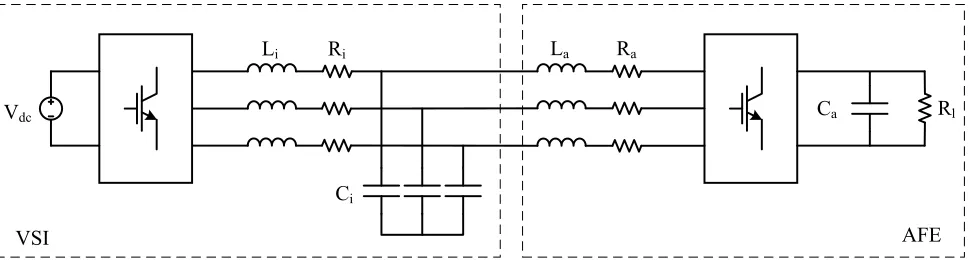
The notional system considered in this paper emulating an embedded power grid is depicted in Fig. 1. It is composed by a Voltage Source Inverter (VSI) fed by a constant DC source and with an LC output filter on the three phase side. An AFE is connected on the VSI output through an inductive filter. On the DC side the AFE is connected to a load through a filtering
L i Ri
Ci
L a Ra
Vdc Ca
VSI AFE
[image:1.612.65.550.581.711.2]Rl
capacitor. A. VSI model
The average model of the VSI system can be easily derived in the dq-reference frame
= + + (1)
where
=
− −1 0
1
0 0
− 0 − −1
0 − 1 0 (2)
=
2 0
0 0
0 2
0 0
=
0 0
−1 0
0 0
0 −1
and
=
(3)
= =
, and are the output filter resistance, inductance and capacitance respectively. is the VSI dc voltage and is assumed to be constant in this work. and are the output inductance current and the output capacitor voltage respectively. is the modulation index, is the AC supply angular frequency and is the current drained by the AFE. Hereafter the subscript d and q denote the d-axis and q-axis of the synchronous reference frame.
B. AFE model: resistive load
The AFE average model in the dq reference with a resistive load on the DC-link side is
and are the input filter resistance and inductance respectively. and are the dc-link voltage and capacitor respectively. is the input filter inductor current, is the dc side resistive load and is the modulation index. In this analysis a DC resistive load has been considered. However the same approach can be applied to different loads, for example
constant power loads. Since the system described by (4)-(5) is nonlinear, it has been linearized resulting in
= + + (6)
where
=
− −
2
− − −
2 3
4 3
4 −
1
(7)
= −
2 0
0 −
2 3
4
3 4
= 1
0
0 1
0 0
(8)
and
=
(9)
= =
The jacobian matrices in (7)-(8) depend from the system states and inputs. The steady state value of system (4)-(5) have been therefore computed [2], resulting in
=
∗ +
∗ =
∗ −
∗
(10)
=
∗ −
2 = ∗ −
8 ∗
3
where the superscript * denotes the reference variable. In addition, it has been assumed that ∗ = 0 and ∗ = 0. Finally
note that system (4)-(5) has 2 steady state points [2]. In Only the one with minimum is reported in (10) and it will be used hereafter.
C. AFE model: constant power load
Another interesting case to consider is the presence of a constant power load on the AFE DC-link side. It is, for example, a good representation of a drive system. To properly model the presence of a constant power load, equation (5) have to be modified accordingly, resulting in:
= − + 3
4 + (11)
This affects also the jacobian matrix (7) that becomes
= − + − 1
2 +
= − − − 1
2 +
(4)
= − 1 + 3
=
− −
2
− − −
2 3
4 3 4
(12)
Also the equilibrium point (10) of the system changes, resulting in
=
∗ −
2 =
∗ −
∗
(13)
=
∗ −
2 = ∗ −
8 3
Also in this case only the equilibrium point with minimum has been reported.
III. CONTROLLER DESIGN
Since the final control goal is to regulate , , and with zero steady state error, systems (1) and (6) have been augmented with integral states. Equation (1) has been therefore rewritten as
= + + (14)
where
=
− −1 0 0 0
1
0 0 0 0
− 0 − −1 0 0
0 − 1 0 0 0
0 −1 0 0 0 0
0 0 0 −1 0 0 (15)
=
2 0
0 0
0 2
0 0
0 0
0 0
=
0 0
−1 0
0 0
0 −1
0 0
0 0
and
= (16)
and are the integral states of and respectively. Similarly, system (6) can be rewritten as
= + + (17)
with
=
− −
2 0 0
− − −
2 0 0
3 4
3
4 −
1
0 0
0 −1 0 0 0
0 0 −1 0 0
(18)
= −
2 0
0 −
2 3
4
3 4
0 0
0 0
= 1
0
0 1
0 0
0 0
0 0
and
= (19)
and are the integral states of and respectively. The state space model of the whole system can be finally obtained merging (14) and (17) resulting in
= + (20)
where
= ′ = ′ (21)
System matrices are defined as
= = 0
0 (22)
with
=
0 0 0 0 0
−1 0 0 0 0
0 0 0 0 0
0 −1 0 0 0
0 0 0 0 0
0 0 0 0 0
=
0 1 0 0 0 0
0 0 0 1 0 0
0 0 0 0 0 0
0 0 0 0 0 0
0 0 0 0 0 0
Model (20) has been derived considering a resistive load on the AFE dc-link side. The derivation of the same model in presence of a constant power load is straightforward using (12) instead of (7).
All the state variables described until now are usually directly measured in this kind of system. It is therefore reasonable to use a state feedback controller to regulate the system. Eq. (20) can be rewritten as
= + +
= − (24)
= +
√
where is the disturbance, ∈ is the performance output and the matrices and are the state and control performance weights. The controller gain matrix can be found solving a H2 optimal control problem [6], i.e. find that minimize the H2 norm of the transfer function from d to z. In time domain, it corresponds to the following optimization problem
min =
+ (25)
If no constraints are imposed to the structure of K, it can be shown that problem (25) is equivalent to a standard LQR problem [7]. In case of designing the control of an embedded power grid, it is however desirable to regulate the different converters independently, in order to avoid the need of additional communication between them. This imposes a predefined structure on the matrix K that forces the control actions of a converter to depend only on its own state. The required gain structure can be written as linear constraints of the optimization problem (25) in the form
∈ (26)
where is the subspace of the admissible gains. For every stabilizing K, the integral in (25) can be computed solving the following Lyapunov equation [8]
− + − = − + ′ (27)
implying
= (28)
The cost function J is a smooth function of K, bounded for every K that makes the closed loop asymptotically stable. It is therefore possible to apply a gradient-based method to find the optimal gain. The cost function gradient is defined as [9]
= + (29)
where L is obtained solving the following Lyapunov equation
− + − = − (30)
Since the cost function (28) is, in general, nonconvex in K, gradient-based approaches can only guarantee the convergence to the local optimal gain.
IV. SIMULATION RESULTS
The proposed method has been tested in simulation. An average model in dq reference frame of the system in Fig. 1 has been firstly implemented using MATLAB. The system parameters used in the simulations are reported in Table I. The gain matrix ∈ has been constrained to have a block diagonal structure of the type
K ∈ 0 0 (31)
where ∈ are the VSI gains and ∈ are the AFE gains. With this constraint it is easily verifiable from (24) that the VSI duty cycles depend only on the VSI states. Similarly, the two AFE gains will be function of the AFE states only. To numerically solve problem (25), HIFOO toolbox [10] has been adopted in this work. This tool uses a BFGS descend technique with a multiple starting point approach to overcome the nonconvexity.
The resistive load case described in section II.B has been tested firstly. The nonlinear system (4)-(5) has been linearized around the nominal working point. Equations (10) have been computed considering ∗= 81 V, ∗ = 270 V and =
24.3 Ω and the complete linearized system has been then computed according to (20). Subsequently the optimal controller gains have been computed as described in Section III.
Fig. 2 shows the step response of the dq average model from a no load AFE dc-bus condition to a full load condition (2 kW). A very fast and stable response can be noted from Fig. 2.
TABLE I SYSTEM PARAMETERS
Parameter Value Unit
2π400 Hz
120e-3 Ω
970e-6 H 31.8e-6 F 200 V
90e-3 Ω
400e-6 H 100e-6 F
Subsequently a switching model has been implemented in Simulink to validate the results obtained with the average system model. A traditional two level voltage source inverter has been used on both VSI and AFE side. The gate signals are generated through Pulse Width Modulation (PWM) with a switching frequency of 20 kHz. Fig. 3 shows the response of the switching system in the same conditions of the simulation tests using the average model, from no load to full load. A very good match between the two dc-link responses can be noted proving the reliability of the average model and the proposed method.
A second model has been realized to test the presented control method in presence of a constant power load on the AFE DC-link side. Also in this case the system has been linearized
[image:5.612.60.288.61.334.2]around the nominal working point described earlier, with a nominal load power of = 2000 W. System and controller parameters used are reported in Table I. It is interesting to notice that the matrix in (12) has an eigenvalue with positive real part, i.e. the open loop system is unstable. The procedure described in section III needs a stabilizing initial value for the gain matrix K that can be complicated to be found for unstable systems. To overcome the problem, in this work the unstructured optimal gain has been firstly computed using a standard LQR approach. Subsequently, the matrix elements that do not respect the constraint (31) have been forced to zero. The resulting matrix has been used as starting point for the optimization algorithm. There is, in general, no guarantee
Fig. 2 – dq average model load step response with resistive load
vs
i d
ut
ie
s
Iidq
[A
]
Vid
q
[V
]
afe duti
es
Iadq
[A
]
Vdc
[V
]
Fig. 3 – abc switching model load step response with resistive load
Iiabc
[A
]
Viabc
[V
]
Iaabc
[A
]
Vd
[image:5.612.329.558.63.341.2]ca [V]
Fig. 4 – dq average model load step response with constant power load
vsi duties
Iidq
[A]
Vid
q
[V]
afe duties
Iadq
[A]
Vdc
[V]
Fig. 5 – abc switching model load step response with constant power load
Iiabc
[A]
Viabc
[V]
Iaabc
[A]
Vd
[image:5.612.326.558.366.555.2] [image:5.612.57.290.371.556.2]the obtained initial gain is stabilizing. However, it has been empirically verified that this strategy works well with the system analyzed in this work. Fig. 4 shows the dq average model response to the connection of a 2 kW constant power load to the AFE DC-link side. Also in this case a very good and stable system response can be noticed. A simulation switching model has been used to validate the results obtained with the average one. Fig. 5 shows the system response to the same test, with a dynamic response very close the one obtained with the average model.
V. CONCLUSION
The paper presents a global optimal approach to tune the power converters controllers of an embedded power grid. A linearized small signal model is used to synthetized the regulators keeping intrinsically in consideration the interactions within the grid. A detailed analysis of the control design problem, including the case of a constant power load has been presented along with a validation of the proposed method using matlab simulations.
VI. ACKNOWLEDGEMENTS
This research work has received funding from the European Union's Seventh Framework Programme (FP7/2009-2018) Clean Sky Joint Technology Initiative. See www.cleansky.eu for details.
VII. REFERENCES
[1] X. Roboam, B. Sareni, and A. D. Andrade, “More electricity in the air: Toward optimized electrical networks embedded in more-electrical aircraft,” Industrial Electronics Magazine, IEEE, vol. 6, no. 4, pp. 6-17, 2012.
[2] H. Kömürcügil, and O. Kükrer, “Lyapunov-based control for three-phase PWM AC/DC voltage-source converters,” IEEE Trans. Power Elect., vol. 13, no. 5, pp. 801-813, 1998.
[3] D.-C. Lee, G.-M. Lee, and K.-D. Lee, “DC-bus voltage control of three-phase AC/DC PWM converters using feedback linearization,” IEEE Trans. Ind. Appl., vol. 36, no. 3, pp. 826-833, 2000.
[4] T.-S. Lee, “Lagrangian modeling and passivity-based control of three-phase AC/DC voltage-source converters,” IEEE Trans. Ind. Electron., vol. 51, no. 4, pp. 892-902, 2004.
[5] B. Wen, D. Boroyevich, R. Burgos et al., “Small-signal stability analysis of three-phase ac systems in the presence of constant power loads based on measured dq frame impedances,” Power Electronics, IEEE Transactions on, vol. 30, no. 10, pp. 5952-5963, 2015.
[6] F. Lin, M. Fardad, and M. R. Jovanovic, “Augmented Lagrangian approach to design of structured optimal state feedback gains,” Automatic Control, IEEE Transactions on, vol. 56, no. 12, pp. 2923-2929, 2011. [7] P. Peres, and J. Geromel, “An alternate numerical solution to the linear
quadratic problem,” Automatic Control, IEEE Transactions on, vol. 39, no. 1, pp. 198-202, 1994.
[8] J. B. Burl, Linear optimal control: H (2) and H (Infinity) methods: Addison-Wesley Longman Publishing Co., Inc., 1998.
[9] T. Rautert, Sachs, Ekkehard W, “Computational design of optimal output feedback controllers,” SIAM Journal on Optimization, vol. 7, no. 3, pp. 837-852, 1997.