Sound source localisation in a
robot
Jasper Gerritsen
Structural Dynamics and Acoustics Department
University of Twente
In collaboration with the Robotics and Mechatronics
department
Bachelor thesis
Abstract
The aim of this thesis is to investigate the possibilites of implementing a beam-former using an 8 microphone array into a robotic head.
Visual interaction between humans and robots is relatively common nowadays, but the topic of interaction via sound is a bit more rare. Also, small microphone arrays that fit inside a robot head are relatively uncommon. For this reason it was decided to investigate the implementation of the technology in this context. This thesis first explains the theory behind beamforming and the influence of scattering on the pressure field. In the next stage the implementation of the technology is considered. A PCB is designed and data acquisition hardware is chosen and put together. Finally the beamforming algorithm is constructed in MATLAB and evaluated.
Contents
1 Introduction 4
2 Theory 5
2.1 Basic principle . . . 5
2.2 Sound waves . . . 6
2.3 System of equations . . . 6
2.4 Measuring the time difference of arrival . . . 8
2.4.1 Delay-and-sum beamforming . . . 8
2.4.2 Cross-correlation beamforming . . . 8
2.5 Sample window . . . 8
2.6 Sample frequency . . . 9
2.7 Number of microphones . . . 9
2.8 Microphone geometry . . . 10
2.8.1 Spatial aliasing . . . 10
2.8.2 Resolution . . . 10
2.9 Scattering . . . 10
2.9.1 Comsol model . . . 11
3 Implementation 14 3.1 Choice of data acquisition hardware . . . 14
3.1.1 DSP . . . 14
3.1.2 Sound cards . . . 14
3.1.3 Digital multitrack recorder . . . 15
3.1.4 USB oscilloscope . . . 15
3.1.5 Comparison . . . 16
3.2 Hardware . . . 17
3.2.1 USB oscilloscope . . . 17
3.2.2 Microphones . . . 17
3.2.3 PCB . . . 18
4 Results 19 4.1 Simulation results . . . 19
5 Conclusions and recommendations 21 5.1 Conclusion . . . 21
5.2 Discussion and recommendations . . . 21
Appendices 23
1
Introduction
Creating a humanlike robot requires lively motions and good looks, but com-munication should not be disregarded. In the field of human-robot interaction creating a friendly robot is an important topic to improve the user’s experience with the robot. This can be achieved by having the robot turn its head towards the person that is speaking.
Interaction between robot and human is usually done via visual sensors. How-ever there are things that cannot be done using only visual sensors. For example it is difficult for a camera to determine which person in the room is speaking. This can however be achieved when the direction of the incoming sound is known.
Here, we investigate the possibility of implementing beamforming in the context of a robot head.
Specifically three aims are addressed:
2
Theory
2.1
Basic principle
This project deals with an inverse acoustic problem, meaning that the effect of the sound is known (measured) and based on these measurements the cause (di-rection) of the sound has to be found. This problem is considered in a context of a conference room where the robot is in the middle of the table and must determine which person is speaking. In speech the frequency spectrum ranges from 200 Hz up to 4000 Hz. [7] The frequencies of interest are in the range of 200-2000 Hz, since frequencies higher than 2000 Hz do not contribute much to the signal.
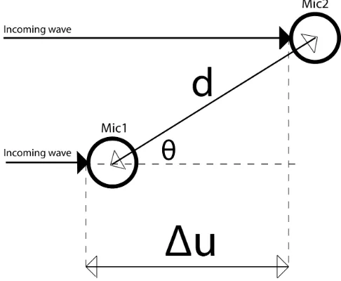
[image:5.612.183.426.336.536.2]Beamforming is a source localization method based on time differences of ar-rival. This is similar to how humans localize sound sources. The basic principle relies on the extra distance the wave has to travel (∆u) to get from one sensor to the next being determined by the angle of incidence of the sound wave,θ.
Figure 1: The basic principle of beamforming
This ∆ugives rise to a time difference of arrivalτ =∆cu = dcsin(θ) between the microphones with c the speed of sound in [m/s].
2.2
Sound waves
Starting from the wave equation,
∂2p ∂t2 =c
2∇2u (1)
this gives solutions for pressure field of a monopole of the form
p(r, t) =f(ωt−kr) (2)
and more specifically
p(r, t) = A
re
i(ωt−kr)
(3)
where A is the complex amplitude of the wave, r is the distance from the source,
k= wc is the wavenumber andω is the angular frequency in [rad/s].
For simplicity in this thesis the sound source is considered to be in the far field. From this it follows directly that the waves are assumed to be planar. In this assumption the wave pattern is governed by only one spatial dimension. In the far field the pressure will be of the form
p(~k·~r, t) = A
re
i(ωt−~k·~r)
(4)
Where~kis the wave vector in the direction of the wave with magnitude|~k|=2λπ in [1/m] and~ris the position vector of the point of interest.
The far field assumption is valid for values of k and r such thatkr1, where k and r are the magnitudes of their corresponding vectors. [6]. This means that for the minimum frequency of interest of 200 Hz the far field starts at
r= 1
k =
1.715
2π = 27cm (5)
Therefore the far field assumption is reasonable in the context of a conference room.
2.3
System of equations
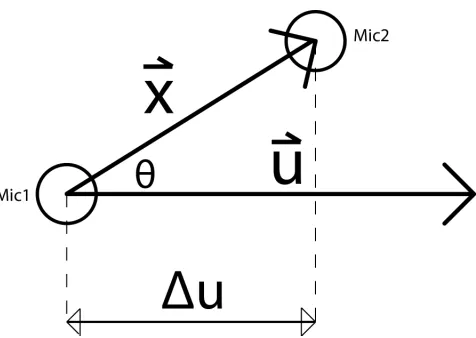
Figure 2: Relevant parameters in a two-sensor array.
In figure 2 the situation is sketched again for 2 sensors now in vector form. The system of equations will be generalized for any number of microphones. Here~uis the unknown incoming sound wave,~xis the position vector from micro-phone 2 relative to micromicro-phone 1. ∆uis to be determined from the beamforming algorithm via ∆u=τ·c where c is the speed of sound.
Three unknowns are identified as the indices of the unit vector of the incoming sound ˆu. This means there need to be at least 3 equations to have a fully determined system.
Now looking at figure 2 the relation between the three relevant parameters can be seen. The scalar projection of~xonto~uis equal to the ∆u. This is shown in equation 6
~
x·uˆ= ∆u (6)
Because there is one reference microphone, in a system with M microphones this gives a system of M-1 equations. Meaning there must be at least 4 microphones for a fully determined system.
x11 x12 x13 x21 x22 x23
..
. ... ...
x(M−1)1 x(M−1)2 x(M−1)3
u1 u2 u3 = ∆u1 ∆u2 .. . ∆uM−1
(7)
Because there is noise in the system the solution will be approximated using the method of least squares. Instead of solving the system
A~u=~b (8)
the following is to be solved:
Here ATA will be a 3×3 matrix and AT~b a 3×1 vector. Notice that this is independent of M, meaning that using more than 4 microphones is not a problem anymore, as the system stays fully determined.
2.4
Measuring the time difference of arrival
In order to find the lag between microphones the signals need to be compared and shifted to find the largest coherence between the signals. This coherence can be measured in a couple of ways.
2.4.1 Delay-and-sum beamforming
First up is delay-and-sum. This method simply adds up the signals for each possible time difference and checks when the output is largest. When this is the case this is the real lag between the signals.
∞ X
m=−∞
|f[m] + g[m+n]| (10)
2.4.2 Cross-correlation beamforming
Secondly there is a small variation to this method where instead of the sum-ming method the correlation function is used. In discrete time the cross-correlation between two functions f and g is defined as stated in equation 11
(f ? g)[n]def= ∞ X
m=−∞
f∗[m]g[m+n] (11)
where n is the lag and m is the time index of the signal. When the correlation value is maximum the lag is estimated to be the real lag. In this definition the discrete inner product is acting on signals with varying lag, therefore it is also known as the sliding inner product.
The cross-correlation method and the delay-and-sum method are of a very sim-ilar nature. The cross-correlation method is used in this project because of its computation time advantage.
2.5
Sample window
The minimum length of the sample is set at 10 periods of the lowest frequency that is to be measured in the speech. As mentioned in section 2.1 the lowest frequency of interest is 200 Hz.
10∗ 1
200 = 50ms (12)
Therefore the sample must be at least 50 ms long.
2.6
Sample frequency
First of all the signal must be sampled at at least twice the highest frequency to be accurately displayed by the signal, also known as the Nyquist frequency. In speech this gives a minimum sampling frequency of 8 kHz. Secondly the signal must have a sufficient amount of samples for the cross-correlation function. This determines the resolution of the algorithm. Say the desired resolution before error margins is 100 regions in a full circle. First the time it takes for the wave to pass the sphere is determined.
0.15
343 = 4.4×10
−4s= 0.44ms (13)
For a resolution of 100 regions per 2 π radians this gives a desired period of 4.4µscorresponding to a sample frequency of 230 kHz.
The resolution of the beamforming algorithm is found to be the limiting factor for the sample frequency. Therefore a sample frequency of 230 kHz is desired.
[image:9.612.199.413.386.532.2]2.7
Number of microphones
Figure 3: Recognition accuracy for different numbers of sensors. [5]
2.8
Microphone geometry
2.8.1 Spatial aliasing
Similar to the Nyquist sampling frequency for the temporal domain, there is also a limit for the spatial sampling frequency. The array requires a maximum spacing between microphones of dmax < λmin2 where λmin is the minimum
wavelength of interest. [4] For simplicity the maximum frequency of interest in this project is set at 2000 Hz. This is possible because the objective is not to display the signals accurately, but rather to be able to compare them. This frequency range contains enough information to do that.
With this maximum frequency in mind the maximum spacing dmax between
microphones is
dmax=
343
2·2000 = 8.58cm (14)
In order to prevent spatial aliasing, the radius of the sphere is therefore set at 7 cm.
2.8.2 Resolution
[image:10.612.234.377.420.552.2]In this application the most important resolution is the azimuth resolution. Therefore most sensors should be placed on the horizontal plane. It is chosen that 6 sensors are spread evenly in a circle on this horizontal plane and 2 sensors are placed on the top and bottom respectively. This is shown in figure 4.
Figure 4: The positions of the 8 microphones
2.9
Scattering
2.9.1 Comsol model
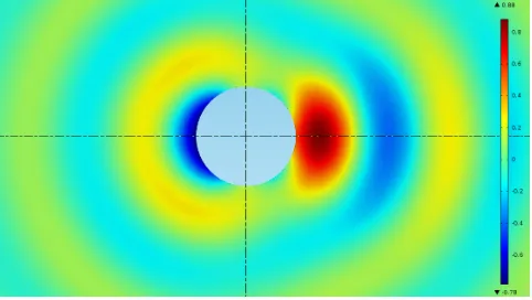
In this model a plane wave of frequency 1000 Hz and an amplitude of 1 Pa is scattered off a sphere of radius .15 m in positive x-direction. The model can be done in 2 dimensions since the problem is symmetrical around the x-axis.
Meshing In order to acquire an accurate solution the maximum element size is set to λ6. This is the standard in acoustics modelling when using second order elements. [1]
[image:11.612.185.428.264.406.2]Results In figure 5 the background field is shown.
Figure 5: Background pressure field in Pa
In figure 6 the scattered field is shown.
Figure 6: Scattered pressure field in Pa
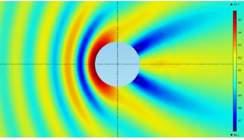
[image:11.612.186.427.466.602.2]Figure 7: Total pressure field in Pa
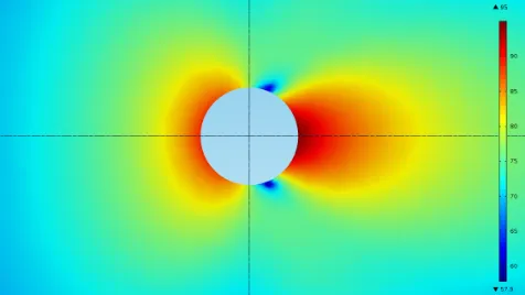
As a measure for the magnitude of the field the sound pressure level (SPL) in dBs is used.
First the scattered field magnitude is shown in figure 8.
Figure 8: Scattered field magnitude in dB
[image:12.612.188.426.350.484.2]Figure 9: Total field magnitude in dB
3
Implementation
3.1
Choice of data acquisition hardware
It is considered to eventually use a Raspberry Pi to process the data, so that the entire hardware can be fit inside the robot head. The hardware is dis-cussed based on properties such as price, timing, size and compatibility with a microcomputer such as the Raspberry Pi.
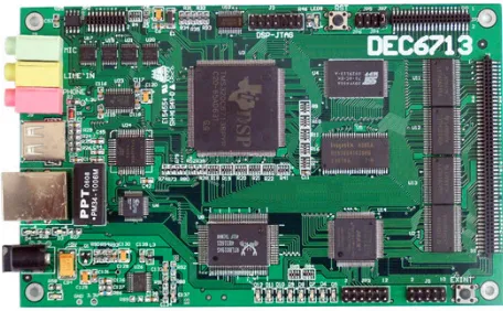
3.1.1 DSP
[image:14.612.192.420.313.454.2]A digital signal processor has the capability to both read out 8 microphones in real-time and process the data immediately. This is however relatively dif-ficult and time-consuming to implement. With this difdif-ficulty also comes great customizability in that the timing settings can be completely controlled.
Figure 10: A digital signal processor
3.1.2 Sound cards
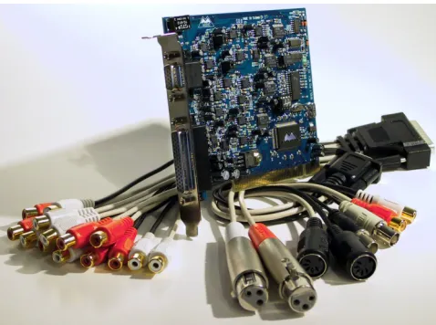
Figure 11: M-audio Delta 1010-LT Sound card
3.1.3 Digital multitrack recorder
This is definitely a very quick and easy solution and very similar to the sound card option. It is however extremely bulky and would not fit inside the robot head.
Figure 12: A multitrack recorder
3.1.4 USB oscilloscope
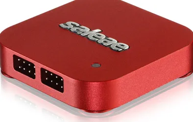
[image:15.612.187.425.407.564.2]is however in fact not that important when creating a humanoid robot, it might even be considered more humanlike. Apart from this it only offers positive points, it is only 5x5x1 cm and has sample frequencies of up to 2.5 MS/s.
Figure 13: Saleae Logic 8
3.1.5 Comparison
Timing Sf Ease of use Price Size Real-time Pi comp. Total
DSP ++ +- - + + + - 3
Sound card + + + + – + - 3
Digital multitrack recorder ++ +- + - – + - 0
USB oscilloscope ++ ++ ++ +- ++ - + 8
3.2
Hardware
[image:17.612.131.475.163.314.2]The hardware setup is shown in figure 14.
Figure 14: The complete setup
In the project a laptop is used to do the data processing in MATLAB. The other components are discussed below.
3.2.1 USB oscilloscope
In choosing the Saleae device there is a lot of room for improvements to the project. The Saleae unit is both very small and has very high sample rates. This makes it ideal to be fit in a robot head and its USB port makes it possible to be combined with a Raspberry Pi microcomputer. There is however currently no support for running the acquisition software on a Raspberry Pi.
Real-time It was mentioned earlier that the USB oscilloscope cannot do real-time acquisition, instead it can only do data-logging. This is because the software is not ready for this. However because the samples necessary for this project are so small that this is not a problem. Logging the sample and exporting it to a .mat file takes approximately 0.3 seconds. Combined with the 0.1 seconds it takes to run the MATLAB code this satisfies the demand of 1 samplewindow per second. Saleae is working on the possibility for real-time input in the future. Sample frequency The 2.5 MS/s sample frequency of the Saleae device is in fact a lot higher than necessary. Luckily there are also lower sample rates available. The sample rate was lowered to 625 kS/s to speed up the sampling process.
3.2.2 Microphones
3.2.3 PCB
[image:18.612.133.479.200.378.2]A printed circuit board is designed in order to power the microphones, amplify them and connect them to the data acquisition unit. The electret microphones are powered via a USB port from the laptop. The amplifier circuit is shown in figure 15.
4
Results
4.1
Simulation results
A MATLAB script has been constructed to reflect the operations as stated in section 2.3. The code can be found in appendix A.
In order to test the program for different SNR ratios, microphone inputs are simulated for a 1 kHz sine wave from the [0, -1, -1] direction. These delays are then attempted to be extracted using the cross-correlation method and the system solution is approximated by least squares.
These solutions are then compared to the real solution for a range of SNRs. First the percentage error in the azimuth direction is constructed:
|∆θ
2π| (15)
[image:19.612.194.406.344.517.2]Then the average value of 30 of these values is taken in order to average out the influence of the noise.
Figure 16: Azimuth error percentages
From figure 16 it is concluded that the algorithm is accurate for SNRs above 10 dB.
Figure 17: Elevation error percentages
As seen in figure 17 the graph is very similar to the first test, but it is worth noting that the algorithm still gives only a 14 percent error for a SNR around 1. This is most likely because the signal is exactly 0 before it starts and after it ends. Therefore it is very easy for the beamformer to determine the correct time difference of arrival.
5
Conclusions and recommendations
5.1
Conclusion
A robust beamforming algorithm was constructed on the basis of a cross-correlation method. Furthermore a literature study was performed on beamforming. A combination of hardware was chosen and put together.
5.2
Discussion and recommendations
In determining the minimum sample frequency it was assumed that the shifting of the signal had to happen simply by shifting one sample over the next. This method sets relatively high demands for the sample rate. Instead a method like a fractional delay filter can be used in order to maximize the resolution. This filter makes it possible to shift a signal by an amount that is not a multiple of the sampling period. This way a lot of data acquisition devices with low sample frequency open up for reconsideration.
The scattering was not included in the final algorithm due to time constraints. Doing this will improve especially the accuracy in the higher part of the fre-quency spectrum. Because the scattering is very much frefre-quency dependent this requires the algorithm to be rewritten to the frequency domain.
References
[1] Acoustic scattering off an ellipsoid. Comsol Multiphysics, Acoustics Module Model Library.
[2] ”saleae hardware”. [Online] Available:
https://www.saleae.com/HardwareTile.
[3] B. D. V. Veen Buckley and K.M. Beamforming: A versatile approach to spatial filtering.
[4] Jacob Benesty S. A. Jacekd Dmochowski. On spatial aliasing in microphone arrays. Signal Processing, IEEE Transactions, vol. 57, 2009.
[5] Thomas M. Sullivan. Multi-microphone correlation-based processing for ro-bust automatic speech recognition. 1996.
[6] Daniel A. Russell Joseph P. Titlow and Ya-Juan Bemmen. Acoustic monopoles, dipoles, and quadrupoles: An experiment revisited. American Association of Physics Teachers, vol. 67, 1999.
Appendix A
Matlab code
function [evalsols, timeDiffs, b] = beamformerleastsq(snr)
%% Initialize
sim = 1; % simulate wave or
% sim = 0; % use actual mics
load('untitled.mat');
sf = analog sample rate hz; % sample frequency
smpNum = num samples analog - 1; % number of samples
%% Coordinates
micPosSph{1} = [0, 0]; % [azimuth, elevation]
micPosSph{2} = [0, pi/2]; micPosSph{3} = [pi/3, pi/2]; micPosSph{4} = [2*pi/3, pi/2]; micPosSph{5} = [pi, pi/2]; micPosSph{6} = [4*pi/3, pi/2]; micPosSph{7} = [5*pi/3, pi/2]; micPosSph{8} = [0, 2*pi/3];
radius = .075;
micNum = length(micPosSph);
micPosCart = cell(1,8); % mics cartesian positions
for k = 1:8
micPosCart{k} = [ radius*sin(micPosSph{k}(2)) * cos(micPosSph{k}(1)), radius*sin(micPosSph{k}(2))*sin(micPosSph{k}(1)),
radius*cos(micPosSph{k}(2)) ];
if k> 1 && k< 8
micPosCart{k}(3) = 0;
end if k == 5
micPosCart{k}(2) = 0;
end end
%% Simulation of wave
c = 343; % speed of sound
simfreq = 1000; realfreq = simfreq/sf;
if sim
% snr = 6; % signal to noise ratio in dbs
noise = ((10ˆ(snr/20))ˆ-1);
% noise amplitude with a signal amplitude of 1
signals = cell(1, micNum); disDiffSim = zeros(1, micNum); input = [0,-1,-1];
for o = 1: micNum
micPosCart{o}/radius) ) / c;
% dot product the unit vectors
nonzerosamples = ceil(smpNum - sf*disDiffSim(o)); signals{o} = cat(2, zeros(1, floor(sf*disDiffSim(o))), sin( (2*pi*realfreq)*(1: nonzerosamples) )) + noise*(-1 +
2*rand(1, smpNum)); % concatenate the zeroes
end end
%% Signals
if !sim
signals = {analog channel 0', analog channel 1', analog channel 2', analog channel 3', analog channel 4', analog channel 5',
analog channel 6', analog channel 7'};
end
% Middle top, circle1, circle2, circle3, circle4, circle5, circle6, middle bottom
%% Cross correlation with respect to mic 1
N = micNum - 1;
% N = N-2;
timeDiffs = zeros(N, 1);
for i = 1: N
[acor,lag] = xcorr(signals{1}, signals{i+1}); % get cross correlation,
acor is correlation value array
% and lag is corresponding lag in samples % positive lag means the middle top mic is % reached later than the outer mic so % all delays are with respect to the % first mic reached.
[~,I] = max(abs(acor)); % index of the highest value of the crosscorrelation
lagDiff = lag(I); % real lag in samples
timeDiff = lagDiff/sf; % real lag in seconds
timeDiffs(i) = timeDiff;
end
disDiffs = timeDiffs * c;
% find the vectors from each mic to the reference mic
micToMic = cell(1, N);
for p = 1: N
micToMic{p} = micPosCart{p+1} - micPosCart{1};
end
%% Do math to find direction
A = zeros(N, 3); b = zeros(N, 1);
for n = 1: N-1 % construct system
for m = 1: 3
A(n, m) = micToMic{n}(m);
end
end
bnew = A'*b; % least squares
Anew = A'*A;
![Figure 3: Recognition accuracy for different numbers of sensors. [5]](https://thumb-us.123doks.com/thumbv2/123dok_us/9820478.483319/9.612.199.413.386.532/figure-recognition-accuracy-dierent-numbers-sensors.webp)