University of Warwick institutional repository: http://go.warwick.ac.uk/wrap
This paper is made available online in accordance with
publisher policies. Please scroll down to view the document
itself. Please refer to the repository record for this item and our
policy information available from the repository home page for
further information.
To see the final version of this paper please visit the publisher’s website.
Access to the published version may require a subscription.
Author(s): Hugo A. van den Berg and Zoe A. Duncombe
Article Title: Eradication-resolution dynamics with stochastic flare-ups
Year of publication: 2010
Link to published article:
http://dx.doi.org/10.1016/j.jtbi.2010.03.010
Eradication-resolution dynamics with stochastic flare-ups
Hugo A. van den Berga,∗, Zoe A. Duncombea
aMathematics Institute, University of Warwick, Coventry CV4 7AL UK
Abstract
In infectious disease as well as in cancer, the ultimate outcome of the curative response, mediated by the body itself or through drug treatment, is either successful eradication or a resurgence of the disease (“flare-up” or “relapse”), depending on random fluctuations that dominate the dynamics of the system when the number of diseased cells has become very low. The presence of a low-numbers bottle-neck in the dynamics, which is unavoidable if eradication is to take place at all, renders at least one phase of the dynamics essen-tially stochastic. However, the eradicating agents (e.g. immune cells, drug molecules) generally remain at high numbers during the critical bottle-neck phase, sufficiently so to warrant a deterministic treatment. This leads us to consider a hybrid stochastic-deterministic approach where the infected cells are treated stochas-tically whereas the eradicating agents are treated determinisstochas-tically. Exploiting the fact that the number of eradicating agents typically decreases monotonically during the resolution phase of the response, we derive a set of coupled first-order differential equations that describe the probability of ultimate eradication as a function of the system’s state, and we consider a number of biomedical applications.
Keywords: Cancer, Infection, Eradication, Extinction bottleneck, T cells, Stochastic processes
1. Introduction
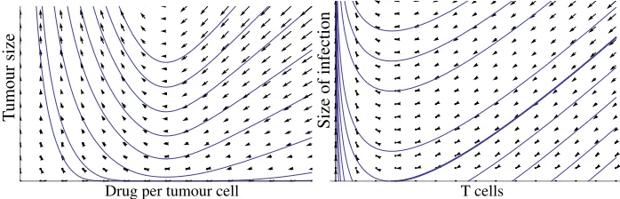
Eradication-resolution dynamics occurs whenever a proliferative disease is being cleared by an agent that is diminishing in numbers. For example, in cancer therapy with immunostimulatory monoclonal antibodies, the antibodies mediate a connection between tumour cells and immune effector cells, and are thus destroyed as the cancer is being eradicated (Bargou et al. (2008); Hudis (2007); Melero et al. (2007)), whereas in a T cell response against a viral infection, the number of T cells drops as the infection is being eradicated (Badovinac et al. (2002), Van den Berg and Kiselev (2004); Harty and Badovinac (2008)). Such eradication-resolution processes are characterised by a dichotomy of outcomes: the disease may be successfully erad-icated, or it might escape, “flaring up” after an initial decrease. This behaviour is illustrated qualitatively in Fig. 1. Starting with a sufficient dosage of the anti-cancer drug, the tumour size initially drops and then increases again as the amount of drug remaining in the system steadily falls (Bargou et al. (2008)). On a deterministic treatment of the problem, the ultimate outcome is always a relapse of the cancer following a temporary remission (Fig. 1, left panel; equations are given below in Section 3.2). For some trajectories, the size of the tumour passes through a minimum that corresponds to just a few cells (or even less than one cell; this is the infamous “attofox” effect). Clearly, the deterministic treatment breaks down at low numbers of tumour cells. Moreover, whether eradication occurs or not depends critically on stochastic effects.
∗Corresponding author
Size
of
infection
T
umour
size
[image:3.612.131.480.113.225.2]T cells Drug per tumour cell
Figure 1: Phase portraits of deterministic examples of eradication-resolution dynamics.
A slightly more complex example is shown in the right panel of Fig. 1 (equations are given and discussed in Section 3.3). Here, both outcomes are possible even in a deterministic treatment: the phase plane is divided into two regions, one in which ultimate eradication is certain and one in which ultimate flare-up is certain. The regions are separated by a critical trajectory which serves as separatrix (the heavy line in Fig. 1). Again, stochastic fluctuations become important as the number of infected cells approaches low numbers, and the probability of eradication would not be expected to jump crisply from 0 to 1 at the deterministic separatrix.
In both examples, it appears that the appropriate approach is to associate with each point in the phase plane the probability that a stochastic trajectory starting at this point will result in eradication. This is a problem of immediate medical interest: when confronted with a tumour mass of a given size, the clinician wants to know the minimal dose that corresponds to a pre-determined likelihood of success. Thus, the evaluation of eradication probabilities from the extent of the disease and a proposed dosage of eradicating agent is central to rational design of treatment.
More realistic deterministic models of tumour growth (including e.g. spatial effects of diffusion limita-tion and vascularizalimita-tion), its induced immune response (including e.g. delays in response and clonal expan-sion), and medical treatment (which may act directly or via immune manupulation) exhibit a richer range of dynamic behaviours (e.g. Araujo and McElwain (2004); de Pillis et al. (2005); Sachs and Hlatky (2010)). Of concern here is the ultimate behaviour of such dynamics, which may be a non-zero equilibrium for the tumour, or some sort of cycling behaviour. In the latter case, the upstrokes of the cycling may be viewed as flare-ups, or the amplitude of the cycle may be small enough that the behaviour is best regarded as oscilla-tions about a non-zero value. But then, from a stochastic point of view, either eradication or flare-up will still be almost certain to occur at some point in time. Of course, as the tumour equilibrium size increases, the probability that either eradication or flare-up occurs during the lifetime of the subject becomes vanishingly small, and thus the need to incorporate a stochastic treatment disappears as well. It is with these caveats in mind that tumour dynamics is regarded as an instance of eradication-resolution dynamics with two possible eventual outcomes.
low-numbers component is treated stochastically and the high-low-numbers component is treated deterministically. The approach is illustrated in the case of a number of typical biological examples in Section 3. A natural extension is considered in Section 4.
2. Eradication probability flow
Deterministic eradication-resolution dynamics can be represented in a fairly general setting by the fol-lowing system of ordinary differential equations:
d
dtx=−µg(x,N)x (1)
d
dtN=ρh(x,N)N−ϑf(x,N)x (2)
wherexis the eradicating agent,Nis the number of pathogenic entities,µ,ρ, andϑare positive parameters,
andg,h, and f are ”functional response” functions, dimensionless multipliers taking values in the
inter-val[0,1], with the stipulation thatg(x,N)6=0 wheneverN>0; thusµ,ρ, andϑare maximum specific rates
of, respectively, agent decay, disease spreading, and eradication. A pair(x(t),N(t))is called aneradication solutionif it satisfies equations (1) and (2) andN(t)→0 ast→∞, whereas(x(t),N(t))is aflare-up solution
if it satisfies equations (1) and (2) and limt→∞N(t)>0.
On the deterministic approach,xandNare both non-negative real numbers. However, since eradication requires thatN pass at least once through a stage whereN∼1, a deterministic treatment is not justified. Also, the deterministic system may not even admit an eradication solution. Accordingly, equation (2) is replaced by a continuous-time Markov chain, withN∈ {0,1,2, . . .}and event rateρh(x,N)N+ϑf(x,N)x for increment/decrement events (N→N±1). The problem is to characterise the functionPN(x), which is the probability of ultimate eradication if the system is started in the state(x,N). The eradication function is determined by the dynamics together with the following boundary conditions:
P0(x) =1 forx≥0 ; (3)
PN(0) =0 forN≥1. (4)
It is assumed that the agent variablexcorresponds to a sufficiently large number of entities to warrant a deterministic treatment (this may not be strictly valid for flare-up solutions in whichx tends to zero as t→∞; however, the behaviour ofxin such cases is not qualitatively important, sinceNwill have passed its low-numbers bottle-neck in the long-time limit).
Letz=x−1andP(z,N)≡PN(x), so that d
dtz=µg(z
−1,N)z (5)
By the above assumptions, for fixed positiveN,zis a monotone increasing function oft, which allows us to use replacetin the continuous-time Markov chain byz. Noting that
P{Nremains constant during an interval of durationδt}
=exp{−(ρh(z−1,N)N+ϑf(z−1,N)z−1)δt}
.
=1−(ρh(z−1,N)N+ϑf(z−1,N)z−1)δt
.
=1−ρh(z
−1,N)N+
we have, by a straightforward application of the law of total probability,
P(z,N)=.
1−ρh(z
−1,N)N+
ϑf(z−1,N)z−1 µg(z−1,N)z δz
P(z+δz,N)
+
ρh(z−1,N)N
µg(z−1,N)zP(z+δz,N+1) +
ϑf(z−1,N)z−1
µg(z−1,N)z P(z+δz,N−1)
δz (7)
forN≥1. Rearranging this probability conservation law, taking the limit
dP(z,N)
dz =δlimz→0
P(z+δz,N)−P(z,N)
δz (8)
and transforming back, we obtain a system of ordinary differential equations for the probability flow:
dPN(x)
dx =
ρh(x,N)N+ϑf(x,N)x
µg(x,N)x pupPN+1(x) + (1−pup)PN−1(x)−PN(x)
(9)
with
pup=
ρh(x,N)N
ρh(x,N)N+ϑf(x,N)x (10)
forN≥1.
One solution is PN(x)≡1 forx>0 andN≥1, i.e. eradication is certain from all starting positions. This would require a jump discontinuity at theN-axis, sincePN(0) =0 forN≥1. To decide whether this is admissible, we must consider the behaviour near theN-axis more carefully. The essential difficulty is that the justification for a deterministic treatment in thex-direction breaks down near theN-axis. Consider momentarily a fully stochastic treatment, in whichxis replaced by a discrete variableX∈N. ForX=1 and
N≥1, the law of total probability then gives the following equation:
PN(1) =ρhNPN+1(1) +µgPN(0) +ϑf PN−1(1)
ρhN+µg+ϑf (11)
(with a slight abuse of notation sinceX, which is absolute-scaled, has replaced ratio-scaledx). Sinceg>0 at X=1 by assumption andPN(0) =0,PN(1)is strictly smaller than 1, which rules out the solutionPN(x)≡1. This accords with the intuitive expectation that for smallx, the probability of eradication decays quickly to zero with increasingN. This argument motivates the following approximate boundary condition for the system with realx:
PN(δx)≡0 forN≥1 (12)
for some small valueδx>0. Heuristically, we can think ofδxas a boundary width satisfying the requirement that the deterministic treatment ofxis admissible forx>δx. Since trajectories that enter the strip
{(x,N)|0<x<δx,N≥0}
cannot leave it, the fact that the ultimate fate of the eradicating agent is discrete absorption, rather than asymptotic decay, does not materially affect the eradication analysis.
To obtain numerical solutions, two truncations are required. The first is the approximate boundary condition (12). Secondly, only finitely many (sayN) equations can be evaluated, prompting the replacementb
ofP
b
N+1(x)byPNb(x)in equation (9), which gives:
dP
b
N(x)
dx =
ϑf(x,Nb)
µg(x,Nb)
P
b
N−1(x)−PNb(x)
0 1 2 3 4 0
20 40 60 80 100
0 1 2 3 4 0
20 40 60 80 100
0 1 2 3 4 5 6 7 0
20 40 60 80 100
T cells T cells T cells
Infected cells
Infected cells Infected cells
Cell
numbers
Cell
numbers
Cell
numbers
Time Time
[image:6.612.98.512.114.222.2]Time
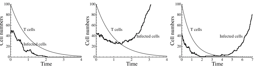
Figure 2: Simulated time courses of the hybrid stochastic-deterministic system derived from eqns (17) and (18), withK=5 andµ=1. The thin line depicts the deterministic dynamics of the T cells (x) and the thick line depicts the stochastic dynamics of the number of infected cells (N).
Numerical solutions must be checked against an unwarranted influence of the chosen values forδxandN.b
The general form of equation (9) is
˙x·∇PN(x) =
∑
∆N
h∆N(x,N) (PN(x)−PN+∆N(x)) (14)
wherex is the deterministic component of the state, evolving with dynamics ˙x, andN is the stochastic component, capable of elementary transitions∆Nwhich occur with hazard rates denoted ash∆N. This is not
in every case the most convenient form of the master equation, but it proves to be useful in eradication-decay dynamics where both components are scalar and (as in the examples of Section 3) ˙xis negative everywhere.
3. Applications
We consider various specifications of the general equations, along with biological interpretations. Each example is designed to illustrate a feature of the present approach.
3.1. Eradication of an intracellular infection by T cells
The first example is defined by the following specifications:
g≡1 h≡1 f = N
K+N
whereKis a positive parameter. Thus
d
dtx=−µx (15)
d
dtN=ρN−ϑ
N
K+Nx (16)
Biologically, this system may be interpreted as follows:Ndenotes the number of cells that have been infected with an intracellular pathogen such as a virus. The proliferation of the infection, at specific rateρ, is stemmed
x x
x x
N N
[image:7.612.124.485.127.223.2]N N
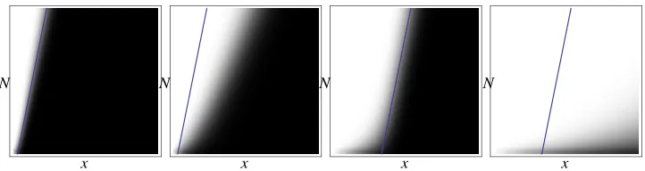
Figure 3:PN(x)for the simple T cell example (white: probability 0; black: probability 1; grey: probability in interval(0,1)). Abscissa
is 0<x≤150, ordinate is 1≤N≤30. Far left:K=5,µ=0.001; middle left:K=5,µ=1; middle right:K=50,µ=0.001; far right:K=50,µ=1. The heavy line is the deterministic null isocline forN.
In this model, the T cells have a standard hyperbolic functional response (Van den Berg and Kiselev (2004)) and decay autonomously and exponentially during the so-calledcontraction phase(Badovinac et al. (2002)). Two parameters can be eliminated by scaling:
d
dtx=−µx (17)
d
dtN=N−
N
K+Nx (18)
(deterministically,Kcould be eliminated as well, but this is not possible for the stochastic treatment sinceN is expressed on an absolute scale).
Hybrid stochastic-deterministic dynamics are obtained by replacing the equation forN by stochastic dynamics as outlined in Section 2; typical simulation results are shown in Fig 2. IfNhas the valueN1>0
on timet1, the probability that the first step change inN(either to N1+1 orN1−1) will occur at a time
greater thant1+τis given by:
exp
−N1τ−
x0N1exp{−µt1}
µ(K+N1)
(1−exp{−µ τ})
(which is obtained by integrating the hazard rateN1(1+x(t)/(K+N1))wherex(t) =x0exp{−µt}, the
solution of eqn (17)). Starting from the same initial conditions, the outcome can be eradication or flare-up (Fig. 2, left and middle panels): the variableNmay spend some time in the low-numbers bottle-neck before the flare-up takes off (Fig. 2, right panel).
Numerical solution of the probability flow equations forPN(x)is straightforward. Representative solu-tions are shown in Fig. 3. When the T cell numbers decay slowly and the saturation parameterK is low, the probability of eradication rises quickly from zero to 1 asxcrosses the deterministic null isocline ofN. Fast T cell decay means that the probability of eradication is virtually zero in the neighbourhood of the deterministic null isocline ofN, and greater T cell numbers are needed to obtain a reasonable probability of eradication. LargerK-values have the effect of blurring somewhat the change-over from low to high probability near theN-null isocline.
x/xc
x/xc
x/xc
x/xc
N N
[image:8.612.121.485.127.226.2]N N
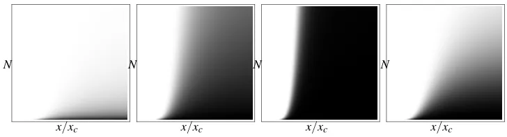
Figure 4:PN(x)for the cancer example (white: probability 0; black: probability 1; grey: probability in interval(0,1)). Abscissa is
0<x/xc≤5, ordinate is 1≤N≤1500;K=50;η=5. Far left:µK/ρ=100,ϑ/ρ=15; middle left:µK/ρ=50,ϑ/ρ=15; middle right:µK/ρ=25,ϑ/ρ=15; far right:µK/ρ=25,ϑ/ρ=10.
and contraction follows a stereotypical or “programmed” response pattern (Badovinac and Harty (2006)): provided the initial expansion delivers a clonal sizex0K+N0 whereN0is the size of the infection at
the onset of the contraction phase, eradication is virtually assured. Against this hypothesis of programmed contraction, one could point to the possibility of a delayed flare-up after the T cells have decayed determin-istically during the low-numbers phase and argue for the hypothesis of regulated contraction, which states that the rate of T cell decay depends, at each moment in time, on the value ofN at that point in time; see Section 3.3, as well as Van den Berg and Kiselev (2004) for arguments in favour of regulated contraction.
3.2. Elimination of a tumour by immunostimulatory antibodies
Consider a tumour, proliferating at specific rateρ>0 and letY denote the molar amount of drug active in the body. The drug is a monoclonal antibody that binds to the surface of the cancer cells, being specific to tumour-specific surface antigens; the Fc tail of the drug molecule binds to the surface of an immune effector cell which kills the cancer cell (Hudis (2007)); alternatively, the drug is a fusion molecule which can engage immune cells that lack the Fcγ receptor, such as T cells (L¨offler et al. (2000)). For the sake of simplicity,
we consider eradication-resolution dynamics for the scenario in which a single dose is administered, and we ignore a multiple dosage or drug infusion regime of administration, which may also be clinically relevant.
Assume that the drug partitions between cancer cells and a fluid phase (blood plasma, tissue fluid) so that a fractionN/(N+K)is bound, whereKis a binding constant. The amount of drug bound per cell may then be defined as follows:
x= Y
N+K . (19)
The effectiveness of the drug is assumed to be a sigmoid increasing function ofx:
d
dtN=ρN−ϑ
N 1+ (x/xc)−η
(20)
whereϑ>ρis the maximum killing rate per tumour cell andxcandηare positive parameters that determine
the shape of the drug effectiveness curve. Drug molecules are assumed to be destroyed when they are bound to a cell that is being destroyed, whereas the free drug molecules disappear with rateµ≥0, thus:
d
dtY=−ϑ
N 1+ (x/xc)−η
x−µ KY
1´104
10 50 100 500 1000 5000
10-5
0.001 0.1
1´104
10 50 100 500 1000 5000
10-5
0.001 0.1
Relapse
probability
[image:9.612.132.473.111.223.2]Scaled dose of drug administered
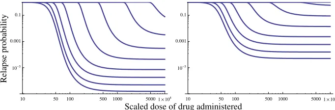
Figure 5: Relapse probability 1−PN(x)as a function of scaled drug doseY/xc;K=50;µK/ρ=25;η=5. Left:ϑ/ρ=10; right:
ϑ/ρ=15. In each panel curves are for (top to bottom):N=3000, 1000, 300, 100, 30, 10, 3, 1.
From equations (20) and (21) we can derive the deterministic component of the eradication-resolution dy-namics:
d
dtx=−µ
K+ (ρ/µ)N
K+N x. (22)
The stochastic component is defined by the event rate
ρ+ ϑ
1+ (x/xc)−η
N
and the probability for the eventN→N+1 is given by:
pup= 1+ (ϑ ρ) (x/xc)−η
−1
. (23)
(We ignore the slight complication thatxis reduced by a factor(K+N)/(K+N+1)wheneverNjumps up; this factor is close to unity for realisticK.)
Qualitatively this example is similar to the previous example, and plots ofPN(x)versusxandNhave the same appearance as those shown in Fig. 4 for the simple T cell model. Deterministically, flare-up (in the case of cancer calledrelapse, which follows the transientremissiondue to the drug’s effects) is assured, whereas stochastically there is a positive probability of eradication provided the dose given is large enough relative to the present size of the tumour. When decay is relatively fast (largeµK/ρ), the probability of eradication
decreases rapidly with tumour sizeN, whereas the relative effectiveness of the drug (ϑ/ρ) determines how
gradual this drop-off in probability is.
Flare-up
probability
x x
x
N N
1 10 100 1000 104
[image:10.612.119.472.126.225.2]10-4 0.001 0.01 0.1 1
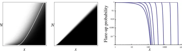
Figure 6: Eradication probabilityPN(x)for the T cells with residual surveillance level example (white: probability 0; black:
probabil-ity 1; grey: probabilprobabil-ity in interval(0,1)). K=50,µ=1. Left: Abscissa is 0<x≤150, ordinate is 1≤N≤30 (the white line is the deterministic separatrix); middle: 0<x≤2000, ordinate is 1≤N≤1000; right: 1−PN(x)as a function ofxfor (top to bottom):
N=3000, 1000, 300, 100, 30, 10, 3, 1.
3.3. T cells with residual surveillance level
According to the simple T cell model of Section 3.1, the T cell number decays to zero. However, it has been observed that a small but functionally significant number of antigen-specific T cells remains after the contraction phase: this is theresidual surveillance levelwhich helps the immune system to suppress re-infection (Harty and Badovinac (2008)). This effect can be explained by the fact that the cytotoxic operation of the T cells tends to damage the T cells themselves as well, so that T cell death is proportional to the rate at which they are themselves destroying infected cells (Xu et al. (2001)). This can be modelled by adjusting the simple model as follows:
g≡ N
K+N h≡1 f =
N
K+N
On this model specification, the T cells stop dying off as soon as eradication has been achieved.
The deterministic model now has a separatrix, as shown in the right panel of Fig. 1, such that trajectories starting to the right of it terminate in a stationary point on thex-axis, whereas trajectories starting to the left exhibit flare up (i.e.x→0 andN→∞ast→∞). Thus, in contrast to the previous two examples, the
Size
of
infection
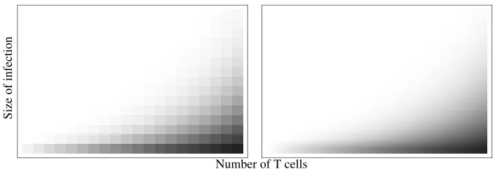
[image:11.612.130.483.102.223.2]Number of T cells
Figure 7: Comparison of fully stochastic (left) and hybrid stochastic-deterministic (right) calculation ofPN(x);θ/ρ=0.05;α=0.01; 1≤X≤20; 1≤N≤15 (white: probability 0; black: probability 1; grey: probability in interval(0,1)).
3.4. Comparison with a fully stochastic treatment
A fully stochastic treatment becomes necessary when the copy number of the eradicating agents becomes small. Consider the following deterministic model:
d
dtX=−αX N (24)
d
dtN=ρN−θX N (25)
whereα,ρ, andθare positive parameters. The eradication probabilities for the stochastic treatment satisfy
the following equations by the law of total probability:
P0(0) =1 and PN(0) =0 forN≥1 (26)
ρPN+1(x)−(ρ+X(α+θ))PN(x) +θX PN−1(x) =−αX PN(X−1) forX≥1. (27) Equation (27) is a non-homogeneous difference equation inN forPN(x)withxfixed andPN(X−1)as a forcing term. Thus, by successively solving forx=1,2,3, . . . the general solution is readily obtained and found to be:
PN(X) = X
∑
ξ=1
X
ξ
α ξ
ρ rξ−1
!X−ξ
κξr N
ξ (28)
where
rξ =ρ+ξ(α+θ)
2ρ 1−
s
1− 4ρ θ ξ
(ρ+ξ(α+θ))2
!
(29)
and the coefficientκξ is defined by the recursion formula:
κξ =1− ξ−1
∑
u=1
ξ
u
αu
ρ(ru−1)
ξ−u
κu forξ≥2 (30)
withκ1=1. The results shown in Fig. 7 suggest that even at low values ofx, the hybrid approach can give
0 5 10 15 0
10 20 30 40 50
Size
of
infection
[image:12.612.130.483.108.224.2]Number of T cells
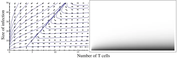
Figure 8: Non-monotone T cell dynamics model for the caseϑ λ<K. Left panel: deterministic phase portrait; right panel: probability of eradication from various starting positions (white: probability 0; black: probability 1; grey: probability in interval(0,1)).
4. Extension to dynamics with recovery of the eradicating agent
In the foregoing sections it was assumed that the eradicating agent (x) decays monotonically. However, in many systems an adaptive response to the flare-up may occur, where the eradicating agent is added or proliferates in response to the pathogen’s escape. By way of example we consider here the following, slightly more complex model of the dynamics of a T cell response:
d
dtx=λx−µ
1− N
K+N
x2 (31)
d
dtN=ρN−ϑ
N
K+Nx (32)
where the T cellsxgrow with specific growth rateλ whereas they disappear by mutual killing in proportion
to the complement of the functional response function (Kottilil et al. (2001); Strasser and Pellegrini (2004); Xu et al. (2001)), which is the usual hyperbolic response (see Van den Berg and Kiselev (2004) for further details on this model). The qualitative behaviour is very different depending on parameter values; when
ϑ λ<K, the T cells are ultimately unable to stem the spread of the infection (Fig. 8), whereas forϑ λ >K,
eradication is assured (Fig. 9). The caseϑ λ =K, while interesting in its own right, is not germane to the
present discussion.
4.1. The caseϑ λ <K
In qualitative terms, the behaviour forϑ λ<Kis somewhat similar to that in the examples of sections 3.1 and 3.2. The eradication probabilities drop off very sharply with increasingNas trajectories become almost certain to converge on a common escape path in the middle of the phase plane (Fig. 8).
Numerical solution of the probability flow equation (9) is slightly more involved. First, the linex=δx
no longer provides a boundary condition; repeating the argument leading to eqn. (11), we now have
PN(1) =
ρhNPN+1(1) +λPN(2) +ϑf PN−1(1)
ρhN+λ+ϑf (33)
0 5 10 15 0
10 20 30 40 50
Size
of
infection
[image:13.612.132.483.111.224.2]Number of T cells
Figure 9: Non-monotone T cell dynamics model for the caseϑ λ>K. Left panel: deterministic phase portrait; right panel: expected time until eradication from various starting positions (white: zero time; black: long time).
equations are numerically stable in the positivex-direction for(x,N)situated to the right ofN= (ϑ/ρ)x−K (part of thexnull isocline) whereas they are stable in the negativex-direction for(x,N)to the left of this line. Moreover, the equations become infinitely stiff near this line. A Picard iteration scheme (Hirsch et al. (2004)) was employed to obtain the solution shown in Fig. 8 (right panel): numerical solutions are generated alternately for the field above and below the nullcline diagonal, each round of the iteration using the solutions on the other side of the nullcline as forcing functions, starting a distanceδxaway from the line to avoid the infinite stiffness (since the stiffness amounts to infinitely rapid equilibration between solutions for adjacent N-values, a very fast relaxation rate nearby achieves practically the same effect). The iteration results in a set of values forPN(x)on the nullcline which serve as consistent boundary conditions for the “forward” and “backward” solutions; in this respect the iterative scheme resembles the shooting technique for nonlinear problems (Burden and Faires (1989)).
4.2. The caseϑ λ >K
We noted in Section 2 that PN(x)≡1 forx>0 andN≥1 solves the probability flow equations, but that the jump discontinuity atx=0 is not allowed by the behaviour near the linex=0. By the argument of Section 4.1, this jump discontinuity is now allowed, and thusPN(x)≡1 is a feasible solution. In the appendix we show that this solution applies whenϑ λ >K. Thus, eradication is certain from all starting positions if the immune efficiency parameters are sufficiently large (although eradication may only be achieved through a series of intermediate flare-ups that are ultimately contained). Instead ofPN (a plot of which would not be informative), we consider the expected time until eradication. Thus, letTN(x)denote the expected time until eradication starting from position(x,N). The derivation is similar; the probability conservation equation (7) now becomes:
T(z,N)=.
1−ρh(z
−1,N)N+ϑf(z−1,N)z−1
µg(z−1,N)z δz
T(z+δz,N)
+
µg(z−1,N)z+ρh(z
−1,N)N
µg(z−1,N)zT(z+δz,N+1) +
ϑf(z−1,N)z−1
µg(z−1,N)z T(z+δz,N−1)
δz. (34)
opposite direction of the phase flow, which is partly due to the deterministic travel time along this trajectory and partly due to the possibility of a quasi-flare-up that will ultimately be contained.
5. Concluding remarks
Hybrid stochastic-deterministic dynamical systems constitute a natural approach, since biological sys-tems are almost invariably essentially stochastic, and one should expect the high-numbers justification for a deterministic treatment to be satisfied for some subset of the system’s components. The usual determin-istic treatment is then seen as a only a special case of the general situation which is a partitioning into a low-numbers component is to be treated stochastically and the high-numbers component can treated deter-ministically (Kiehl et al. (2004); Wilkinson (2006)). Simulation of such hybrid systems is perfectly straight-forward (Alfonsi et al. (2005)); since the hazard rates generally co-depend on the deterministic component, it is necessary to integrate this time-varying hazard in order to realise the time till the next transition in the stochastic component (this time interval being a random variable).
We focussed on rather simplified biomedical examples of eradication-decay dynamics; other examples may be found in pest control, epidemiology, and pharmacodynamics. The key quantity of interest is the probability of eradication (or its complement, the risk of flare-up) starting from a given quantity of eradi-cating agents. In T cell dynamics, this quantity is the maximal expansion of the responding clonotype; in oncology, it is the dose of drug administered. In both cases, dynamics may be considerably more com-plicated. Also, probability of flare-up is not the only clinical outcome marker (although it is an important one); the drug administration regime may be chosen to minimise a cost functional that takes into account the hazard rates for various morbidities associated with the tumour mass as well as the drug itself (side effects). To calculate the optimal drug dosage in this case requires an optimal-control approach, such as the one taken in Van den Berg and Kiselev (2004).
Acknowledgement. The authors express their gratitude to an anonymous reviewer for providing insightful
Alfonsi, A., Canc`es, E., Turinici, G., Di Ventura, B., Huisinga, W., 2005. Adaptive simulation of hybrid stochastic and deterministc models for biochemical systems. ESAIM: Proceedings, 1–10.
Araujo, R. P., McElwain, D. L., 2004. A history of the study of solid tumour growth: The contribution of mathematical modelling. Bull. Math. Biol. 66 (5), 1039–1091.
Badovinac, V. P., Harty, J. T., 2006. Programming, demarcating, and manipulating CD8+T-cell memory. Immunological Reviews 211, 67–80.
Badovinac, V. P., Porter, B. B., Harty, J. T., 2002. Programmed contraction of CD8+T cells after infection. Nature Immunol. 3, 619 – 626.
Bargou, R., Leo, E., Zugmaier, G., Klinger, M., Goebeler, M., Knop, S., Noppeney, R., Viardot, A., Hess, G., Schuler, M., Einsele, H., Brandl, C., Wolf, A., Kirchinger, P., Klappers, P., Schmidt, M., Riethm¨uller, G., Reinhardt, C., Baeuerle, P. A., Kufer, P., 2008. Tumor regression in cancer patients by very low doses of a T cell–engaging antibody. Science 321, 974–977.
Berg, H. A. van den., Kiselev, Y. N., 2004. Expansion and contraction of the cytotoxic T lymphocyte response—an optimal control approach. Bull. Math. Biol. 66, 1345 – 1369.
Burden, R. L., Faires, J. D., 1989. Numerical Analysis, 4th Edition. PWS-Kent Publishing Company, Boston.
de Pillis, L. G., Radunskaya, A. E., Wiseman, C. L., 2005. A validated mathematical model of cell-mediated immune response to tumor growth. Cancer Research 65, 7950–7958.
Harty, J. T., Badovinac, V. P., 2008. Shaping and reshaping CD+T-cell memory. Nature Rev. Immunol. 8, 107–119.
Hirsch, M. W., Smale, S., Devaney, R. L., 2004. Differential Equations, Dynamical Systems, and an Intro-duction to Chaos. Elsevier.
Hudis, C. A., 2007. Trastuzumab — Mechanism of action and use in clinical practice. New Engl. J. Med. 357, 39–51.
Karlin, S., Taylor, H. M., 1975. A First Course in Stochastic Processes, 2nd Edition. Academic Press.
Kiehl, T. R., Mattheyses, R. M., Simmons, M. K., 2004. Hybrid simulation of cellular behavior. Bioinfor-matics 20, 316–322.
Kottilil, S., Bowmer, M. I., Trahey, J., Howley, C., Gamberga, J., Granta, M. D., 2001. Fas/FasL-independent activation-induced cell death of T lymphocytes from HIV-infected individuals occurs without DNA frag-mentation. Cell. Immunol. 214, 1–11.
L¨offler, A., Kufer, P., Lutterb¨use, R., Zettl, F., Daniel, P. T., Schwenkenbecher, J. M., Riethm¨uller, G., D¨orken, B., Bargou, R. C., 2000. A recombinant bispecific single-chain antibody, CD19×CD3, induces rapid and high lymphoma-directed cytotoxicity by unstimulated T lymphocytes. Blood 95, 2098–2103.
Melero, I., Hervas-Stubbs, S., Glennie, M., Pardoll, D. M., Chen, L., 2007. Immunostimulatory monoclonal antibodies for cancer therapy. Nature Rev. Cancer 7, 95–106.
Strasser, A., Pellegrini, M., 2004. T-lymphocyte death during shutdown of an immune response. TRENDS Immunol. 25, 610–615.
Wilkinson, D. J., 2006. Stochastic Modelling for Systems Biology. Chapman and Hall.
Xu, X.-N., Purbhoo, M. A., Chen, N., Mongkolsapaya, J., Cox, J. H., Meier, U.-C., Tafuro, S., Dunbar, P. R., Sewell, A. K., Hourigan, C. S., Appay, V., Cerundolo, V., Burrows, S. R., McMichael, A. J., Screaton, G. R., 2001. A novel approach to antigen-specific deletion of CTL with minimal cellular activation using
Appendix: Eradication probabilities for the non-monotone T cell dynamics model
We consider the system
d
dtx=λx−
1− N
K+N
x2 (.1)
d
dtN=N−ϑ
N
K+Nx (.2)
which is a scaled version of the system defined by equations (31) and (32). Deterministically, the stationary point(x,N) = (λ,0)is a global attractor ifϑ λ>K, whereas stochastically, flare-ups may occur, but eventual eradication is assured. To prove this, letRdenote the region
Rdef
= n(x,N)|x>λ & 0<N≤Kx
λ−1
o
and define
e
N(x)def=entKx
λ −1
(.3)
where ent(·)is the entier functionR→Nwhich rounds its argument down to the nearest integer. Suppose
that every trajectory must eventually (re)visitR. Since the downward jump probabilities are strictly positive, the probability that the phase point, starting fromNe(x)for some finitex, on its next exit fromR does so
by eradication (i.e. absorption toN=0) is bounded away from zero. Furthermore, sincexis monotonically decreasing for phase points inR, a trajectory traversingR must eventually exitR, either by eradication or into the region whereN>Ne(x). Therefore the probability that a trajectory starting from an arbitrary
point(x,N)withx>0,N>0 will exhibitnexits fromRwithout eradication is bounded above by(1−δ)n
for someδ >0. Since this probability tends to zero asn→∞, every trajectory must eventually exitRby eradication.
It remains to show that every trajectory must enterR. Consider a trajectory starting from a phase point outside ofR, and letuN(x) denote the probability of absorption into R starting from the point (x,N). Also, letvN−
e
N(x)(x)denote this probability whenxis held fixed. Since clearlyuN(x) =1, we havev0(x) =1. Suppose that the trajectory never entersR. Along such a trajectory,xincreases monotonically, either without bound or, ifNremains constant from some point in time onwards, bounded by a finite value. However, the latter possibility is ruled out since the jump probabilities are nonzero. Thusxmust tend to infinity along a trajectory that never entersR. This fact, together with the dependence of the jump probabilities onx, implies thatuN(x)≥vN−Ne(x)(x). It therefore suffices to show thatvN−Ne(x)(x)→1 for allN≥1 asx→∞. This is
the case precisely when the following quantity diverges:
S(x)def= ∞
∑
i=1
i
∏
j=1
ϑx
K+Ne(x) +j !
(.4)
(see e.g. (Karlin and Taylor, 1975, p. 147)). To establish this divergence, letm(x)be a functionR→Nsuch
that
m(x)<ϑx−Ne(x)−K and
m(x)→∞
m(x)/x→0 asx→∞
and let
r(x)def=Ne(x)−K
x
λ −1
By definition, 0≤r(x)<1 and thus limx→∞r(x)/x=0. The sumS(x)can be bounded below by a geometric
sum:
S(x)≥ ∞
∑
i=1
i
∏
j=1
ϑx
K+Ne(x) +i !
= ∞
∑
i=1
ϑx
K+Ne(x) +i
i
≥
m(x)
∑
i=1
ϑx
K+Ne(x) +i
i
≥
m(x)
∑
i=1
ϑx
K+Ne(x) +m(x)
i
= ϑ λ
ϑ λ−K−λ(m(x) +r(x))/x
ϑ λ
K+λ(m(x) +r(x))/x
m(x)
−1
!
(.6)