WORKING PAPERS SERIES
WP01-14
The Asset Allocation Decision
in a Loss Aversion World
The Asset Allocation Decision in a Loss
Aversion World
Soosung Hwang
Department of Banking and Finance,
City University Business School
Stephen E. Satchell
1Faculty of Economics and Trinity College,
Cambridge University
June 6, 2001
1Corresponding Author. Faculty of Economics and Politics, Cambridge
Abstract
The purpose of this paper is to derive explicit formulae for the asset allo-cation decision for the loss aversion utility function proposed by Kahneman and Tuversky. We show that these utility functions exhibit constant absolute risk aversion. We also give analytic results which interpret the assumptions of risk-aversion with respect to gains but risk-a!ection with respect to losses in terms of changes of the optimal investment of equity when the proba-bility that equity outperforms cash goes up. For the Knight, Satchell and Tran (1995) family of distributions, it is straightforward to derive closed form expressions for the optimal portfolio weights in all cases. Using UK and US data, we confirmed that the values of the parameters in the loss aver-sion function suggested by many previous studies are compatible with the observed proportions held in equity in both the UK and the US. The distri-butional assumptions are not innocuous. However, whilst modelling upside and downside returns by gamma distributions leads to plausible results, mod-elling upside and downside by truncated normals does not.
1
Introduction
Modern finance theory starts from a set of normatively appealing axioms about individual behavior. That is, people are assumed to be risk-averse expected utility maximizers and make rational choices based on rational ex-pectations. However, the rational paradigm has been criticized by many behavioral economists and psychologists such as Kahnemann and Tversky (1979) and De Bondt and Thaler (1985).
In particular, dissatisfaction with power utility has been a re-occuring theme in modern financial economics. From the equity premiumm puzzle to the inability to explain the presence of gambling and holding insurance simultaneously, power utility’s faults are numerous and well-documented; see Mehra and Prescott (1985) and Campbell and Viceira (1999) for exam-ple. New alternatives built around power utility have been put forward; loss aversion (Kahnemann and Tversky, 1979, 1992) and disappointment aversion (Gul, 1991 and Ang, Bekeart and Liu, 2000) may work better to name but some of the alternatives.
The purpose of this paper is to concentrate on loss aversion (LA) utility, first put forward by Kahnman and Tversky (1979, 1992) and used, among others, by Barberis, Huang and Santos (1999), Berkelaar and Kouwenberg (2000a, 2000b), and solve the asset allocation problem for an investor with LA utility in a one period world. In doing so, we revisit the two piece utility functions of Fishburn and Kochenberger (1979) who put forward this structure of utility as an example of conventional expected utility theory.
For a very broad family of distributions, the KST family, see Knight, Satchell and Tran (1995), it is possible to derive closed form expresssions for the optimal proportion of wealth held in equity. Although one can compute the optimal proportion fairly easily using numerical methods, the benefits of explicit formulae are self-evident. Furthermore, inspection of the results gives us a better understanding of the factors driving equity investment and the delicate nature of the assumptions governing upward and downward risk tolerance.
In section two, we present details of both the LA utility being consid-ered and the KST distribution. Results are presented in section three, an application to UK equity follows in section 4 whilst section 5 concludes.
2
The Optiml Portfolio with Loss Aversion
benchmark. Defines gains X=W !B, then LA utility is defined as
u(X) = X
v1
v1
, if X >0, (1)
= !!(!X)
v2
v2
, if X "0,
where the parameters v1,v2 and! are assumed positive.
It is possible to distinguish several cases. The first case is that0< v1 <1,
0 < v2 < 1. In this case u(.) is ’risk averse’ with respect to gains since
u!!(X) = (v1 ! 1)Xv1"2 which is negative. However, u(.) is risk loving
with respect to losses since u!!(X) = !!(v
2 !1)(!X)v2"2 which is positive.
Another possibility studied in the literature is to let vi = 1, i = 1 or 2, so
that u(.) could be risk neutral with respect to gain or loss. For example, Kahnemann and Tversky (1979) use v1 =v2 = 0.88 and! = 2.25, Benartzi
and Thaler (1995) use v1 = v2 = 1 and ! = 2.25, Ang, Bekeart, and Liu
(2000) use v1 = v2 = 0.88 and a range of ! values, although some of these
applications are for multi-period optimisations rather than the one-period problem we consider here.
However, other cases could be of interest. If v1 > 1 and v2 > 1, then
the investor is risk loving with respect to gains whilst risk averse to losses. Which of these alternatives is the more plausible is not obvious. Several risk control strategies, prevalent in the market, capture some aspect of these alternative cases. For example, a stop-loss strategy controls downside risk and is presumably consistent with v2 > 1. A take-profit strategy controls
upside risk and might be consistent with v1 < 1. Therefore, it is not clear
on a prior grounds or observed behaviour whether 0 < v2 < 1, v2 > 1, or
v1 >1, and so we include all possibilities. These appear to be no theoretical
results in the literature that support any of the di!erent assumptions aboutv1
andv2. However, Fishburn and Kochenberger (1979) present some empirical
evidence ! > 1 and that 0 < v1 < 1 and 0 < v2 < 1. They also refer to
other papers that present empirical support of these assumptions, namely investors are risk-averse for gains and risk-loving for losses. In choosing B it is customary to let B equalW0 orW0(1 +rf) whererf is the riskless rate of
return and we shall adapt the latter approach.
Asset allocation problems consider optimal portfolios taken over a small number of asset classes. Suppose that there are two assets; a riskfree as-set and a risky asas-set whose returns are denoted by rf and r, respectively.
Denoting " to be the proportion held in equity, then final wealth is
W = W0(1!")(1 +rf) +W0"(1 +r) (2)
where B =W0(1 +rf)andy=r!rf is the excess return of the risky asset,
and thus X =W0"y. In what follows, we implicitly assume that " # 0, i.e.,
short sales are not allowed.
In the following theorem, we show that under some condition, any utility function of W !B becomes CARA class of utility functions.
Theorem 1 Suppose u is a utility function of the form u(W ! B) where
B =W0(1 +rf) and u does not depend upon W0 in any other way. Then it
follows that u is CARA.
Proof. For an investor whose utility function isu(W!B), the problem is
to solve
max
! E(u("W0(r!rf))).
The first order conditions are, putting y=r!rf andh="W0
E(u!("W0y)W0y) = 0
or
E(u!(hy)y) = 0.
The solution h! depends only upon the form of u and the distribution of y
but not W0, since by assumption u does not depend on W0. So we find that
!
"W0 =h! and result is proved.
Remark 1 Although this may appear restrictive, it is quite easy to reparametrise
this problem so that the utility function exhibits non-constant absolute risk aversion. See Pedersen and Satchell (2001) for details of this approach. In the context of this problem, let
u(W !B) = u1(W !B) if W #B
= !!u2(B !W) if W < B,
where ! is some positive constant. If we let ! = !(W0) and if !" is the
optimal solution to A, then !" is, typically, decreasing in !. The dynamics of
!
" or !"W0 with respect to W0 can be deduced from the relationships !" = !"(!)
and ! =!(W0).
The optimal portfolio can be obtained with an appropriate choice of ".
Let u+ =E(yv1|y > 0), u" =E((!y)v2|y <0), p=prob(y > 0). Since X in
equation (1) is equivalent to W0"y, expected utility ULA is given by
ULA =
1
v1
(W0")v1u+p!
!
v2
Thus the first derivative with respect to " is
ULA! =Wv1
0 p"
v1"1u+
!!Wv2
0 (1!p)"
v2"1u". (3)
Inspection of (3) shows that if v1 = v2, the optimal solution for " is 0
if Wv1
0 u+p < !W0v2u"(1! p), or $ if W0v1u+p > !W0v2u"(1 !p). If the
inequality is an equality, " is indeterminate sinceU!
LA is zero.
SettingU!
LA = 0 and solving for the case v1 %=v2, we see that
" =
"
u+pWv1"v2
0
!u"(1!p)
# 1
v2!v1
(4)
= 1
W0
"
u+p
!u"(1!p)
# 1
v2!v1
and
ln"= 1
v2!v1
ln(u+p)! 1
v2!v1
ln(!u"(1!p)) (5)
when W0 = 1.
In equations (4) and (5) the solution for" is general. We have, therefore, the following proposition.
Proposition 2 If the investor has an LA utility function with v2 %= v1 and
benchmark B =W0(1 +rf), then the optimal equity investment proportion "
in equation (4) can be obtained for any arbitrary probability density function. Furthermore, "W0 is constant so we have constant absolute risk aversion.
Proof. For the first part, the proof is given above. The second argument
can be proved with equation (4), since the dollar amount in equity is "W0,
and,
"W0 =
"
u+p
!u"(1!p)
# 1
v2!v1
,
which is independent of W0. QED.
Proposition 3 If the investor has an LA utility function with v2 %= v1,
B = W0(1 +rf), and the proportion of wealth held in equity is an
increas-ing function of the probability that equity outperforms cash, then we have
v2!v1 >0.
Proof. Since the proportion of wealth in equity goes up with the probability
of a gain, the partial derivative ofln" with respect tolnpshould be positive, i.e., "ln!
"lnp >0. Thus, from equation (5),
#ln" #lnp =
1
(v2!v1)(1!p)
The condition that satisfies the above equation is v2!v1 >0. QED.
Proposition 2 is a sensible constraint since it implies that the proportion of wealth held in equity goes up if the probability of a gain goes up (ceteris paribus, other than that the probability of a loss goes down automatically). We now ask what behaviour is ruled out? For example, if v1 >1andv2 <1
so that we are risk loving for both gains and losses, this would be ruled out by the obvious constraint. If v2 >1 so that we are risk averse for losses we
can still be risk loving for gains as long asv1 < v2. Obviously risk neutrality
for losses and risk loving for gains is also excluded.
Remark 2 In the general case, if the investor is risk averse for gains and
losses, then v2 > 1, v1 < 1 and v2 !v1 is positive, in this case ""lnlnu!+ is
positive and ""lnlnu!! and
"ln!
"ln# are negative.
Remark 3 If W0 is set to 1 and 0<"<1, then any positive v2!v1 would
imply from (4) that u+p <!u"(1!p).
3
Empirical Tests
In this section, we suggest appropriate sets of v1, v2 and " for the UK and
US markets under the assumption that the excess returns of risky asset in (2) are normally distributed. However, in many cases, normality is not an appropriate assumption. As an alternative to the normal distribution, we use the KST distribution. Some additional explanation on our distributional assumptions and our empirical results follow.
3.1
KST and Normal Distributions
Since the optimal " can be obtained with any distribution, we can calculate the optimal " for the most widely used distribution, the normal distribution, and an alternative, the KST distribution which we define next. Let yt be the
excess return at time t,
yt =µ+$1tzt!$2t(1!zt), (6)
whereµis the mean ofyt,andztis a binary indicator variable with probability
p, and $1t and $2t are independent non-negative randon variables. Then, the
pdf of yt is,
pdf(yt) ={
pf1(yt!µ) for yt#µ
where f1 and f2 are pdf’s. In our study, µ is set to zero because the
expec-tations u+andu" are conditional ony
t#0 oryt<0.
The first case we consider is the KST distribution. The KST distribution is designed to capture the asymmetry in upward and downward asset returns. The pdf’s of the KST distribution, f1 and f2, are assumed in this paper to
be the scale Gamma distribution;
fi(x) ={
$!i i x!i!1
!(%i) exp(!%ix) forx >0
0 otherwise, (8)
for i =1 and 2. Thus, when p= 1/2,%1 =%2 and&1 =&2, the pdf becomes
symmmetric. Although in this paper, we assume that rt isiid, it is
straight-forward to extend this model to make µ time dependent and let zt follow a
Markov process. See Bond (2001) or Damant, Hwang, and Satchell (1999) for example.
With the KST distribution, we can obtain analytical results for u+ and
u" with the KST distribution. As explained above, the KST distribution
provides us with a closed form solution for u+ and u" in (4) as well as capturing the asymmetric properties of asset returns. Note that in the case of the gamma distribution,
u+ = E(yv1
|y >0) =
$ #
0 y
v1f
1(y)dy
=
$ #
0 y
v1%
%1
1 y%1"1
!(&1)
exp(!%1y)dy
= !(v1+&1)
%v1
1 !(&1)
$ #
0
%v1+%1
1 yv1+%1"1
!(v1+&1)
exp(!%1y)dy
= !(v1+&1)
%v1
1 !(&1)
,
since
$ #
0
%v1+%1
1 yv1+%1"1
!(v1+&1)
exp(!%1y)dy= 1.
Likewise
u" = E((!y)v2
|y <0) =
$ #
0 y
v2f
2(y)dy
=
$ #
0 y
v2%
%2
2 y%2"1
!(&2)
exp(!%2y)dy
= !(v2+&2)
%v2
2 !(&2)
since
$ #
0
%v2+%2
2 yv2+%2"1
!(v2+&2)
exp(!%2y)dy= 1.
Therefore, for the KST distribution,
ULA=p
(W0")v1
v1
u+!(1!p)!(W0")
v2
v2
u",
where
u+ = !(v1+&1)
%v1
1 !(&1)
,
u" = !(v2+&2)
%v2
2 !(&2)
.
The second case we consider is the frequently used normal distribution which is used for comparison purpose in this study. The normal distribution function for a variable x is
f(x) = &1
2'(exp
%
!(x!µ)
2
2(2
&
for x >0 (9) whereµand( are mean and standard deviation of the variablex. Note that in the above normal distribution, we do not use di!erent paramaters for the negative and positive returns and thus it does not capture the asymmertic property of the asset returns. In addition, analytical derivation for u+ and
u+ is di"cult and in this study, we calculate them numerically. It is worth
noting that
u+=
$ #
0 y
v1& 1 2'(1
exp
%
!(y!µ1)
2
2(2 1
&
dy
and
u"=
$ 0
"#(!y) v2& 1
2'(2
exp
%
!((!y)!µ2)
2
2(2 2
&
dy
3.2
Empirical Testing
For the two distributions above, we use UK and US financial data to capture the asset allocation decisions of typical UK and US investors. That is, we use equation (4) to obtain sensible sets of v1 and v2 for a given level of the
investment proportion on risky assets.
di!erent asset classes which need a great deal of data and information. In-stead, as discussed earlier, we shall concentrate on a stripped-down version of the problem, namely, two asset classes. This simplified version which consists of a riskfree asset and an equity (risky asset) is consistent with the setting we used above for the optimal portfolio with loss aversion. Note that the investment proportion in domestic and foreign equity in 1993 was 83% for large pension funds in the UK, while in the USA it was 46%1.
For the riskfree and equity, we use the three month UK treasury bill and the FT All-share for the UK market and the three month US treasury bill and the S&P500 for the US market. Thus in the above loss aversion utility the benchmark is represented by the three month treasury bill interest rate. The monthly treasury bill rate and the market index return from January 1980 to February 2001 for a total of 254 monthly observations are used. In addition, to investigate time-varying properties of the returns, we divide the entire sample period into two arbitrary sub-samples; the first sub-sample from January 1980 to December 1989 and the second sub-sample from January 1990 to February 2001.
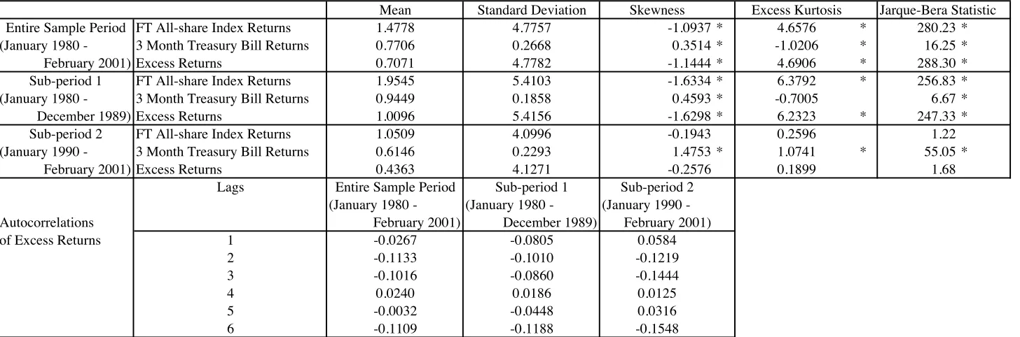
We first report the statistical properties of the data in table 1. The mean and standard deviation of the UK returns are similar to those of the US returns. Because of last several years’ high economic growth in the US, the US market outperformed the UK market in the second sub-sample period. The table also shows that the UK market returns are more negatively skewed and fat-tailed than the US market returns. But most of the non-normality in the UK market comes from the first sub-sample period, and during the second sub-sample period, the US market is more skewed and fat-tailed than the UK market.
Overall, the monthly excess returns are not normal both in the UK and US markets; Jarque-Bera statistics show that most excess returns are non-normal. As is well-known, when empirical distributions are not normal, any results obtained with the assumption of normality may be wrong. We need to model the impact of asymmetry and fat-tail in returns.
We first use the double gamma distribution as in (8) proposed by KST. The double gamma distribution can be combined with the regime switching model introduced by Hamilton (1989), if we assume that the binary indicator variable zt in equation (6) follows a two-state Markov process. In this case,
the probability density function becomes complicated. See KST for further discussion on regime switching double gamma pdf. The autocorrelation co-e"cients reported in table 1 suggest that the excess returns are not serially
1These numbers were found in the following unpublished mimeos; MERCERS,
correlated. Thus, we do not pursue this complicated version any more here. Table 2 reports the estimates of KST parameters with the excess returns forµ= 0. All estimates are significant and similar to those reported in KST; large values of %1 and%2, and&1 >1and&2 >1. We can test symmetry by
the hypothesis %1 =%2, and&1 =&2. During the first sub-period, the excess
returns seem to be asymmetric, but the estimates of the second sub-period show that excess returns may be symmetric. In addition, the density has maximum value at(&i!1)/%iwhen&i >1.In our case, the estimates of&iare
all larger than one and thus has miximum value; for example, for the second sub-period in the UK market, the conditional densities for both positive and negative excess returns have maximum value at (&!1!1)/!%1 = (1.244!
1)/40.403 = 0.006, and(&!2!1)/!%2 = (1.109!1)/33.002 = 0.003, respectively.
In addition, the likelihood ratio tests with the maximum likelihood values (not reported) suggest that there is no significant di!erence between the first and the second sub-periods. Thus we use the estimates obtained with the full samples.
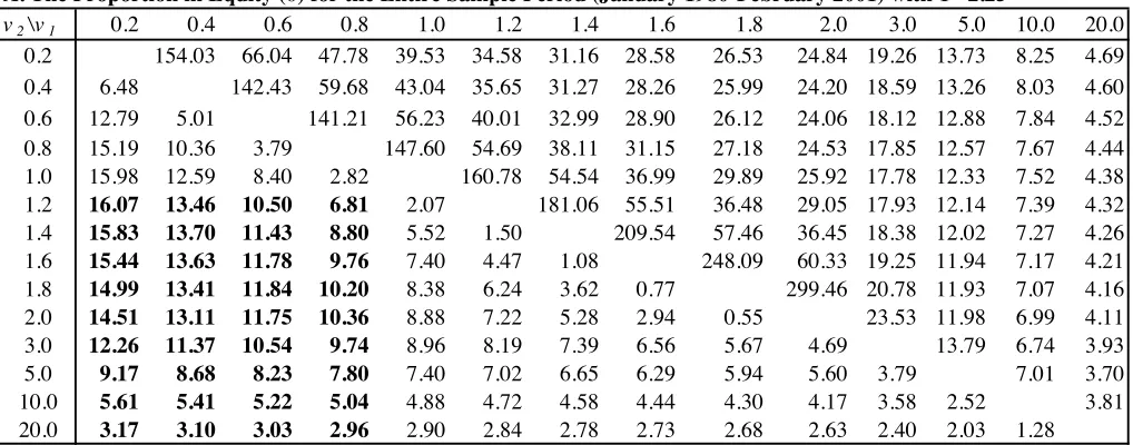
Using the paramater values estimated in table 2, we first calibrated the values of " for given values ofv1, v2, and!.The ranges of v1 andv2 were set
from 0.2 to 20, respectively, and ! was set to 1.5, 2.25, and 3. We used the Newton-Raphson algorithm on equation (4) with the assumption of W0 = 1
to calculate ".
Table 3 shows the investment proportion, ", for the settings in the UK market. We first investigate the results for the case of ! = 2.25 in panel A, which shows that when v1 > v2, the values of " were at least more than
2000%, which is too large to accept. The results confirms the admissible ranges suggested in Proposition 2. However, for the investors who are risk averse for gains and losses as in Remark 1, we still have too large investment proportions, i.e., 300% to 1600%. See bold numbers in panel A of table 3. The table also suggests that whenv2!v1 >0andv1 andv2are close to each other,
it is possible to explain the UK and USA investment proportions in equity (i.e., 83% and 46% for large pension funds in the UK and USA, respectively).2 These results are roughly consistent with other multi-period studies where
v1 andv2 are assumed to have the same value. See Kahnemann and Tversky
(1979), Ang, Bekeart, and Liu (2000) and Benartzi and Thaler (1995), for example. In addition, as expected, comparing panel A with panels B and C shows that when the penalty to loss becomes larger, ! = 3, investment proportions on equity decrease, and vice versa.
We now further investigate what may be appropriate sets ofv1 andv2 to
2We do not report the USA cases which are similar to those of the UK. The results in
explain the UK and USA markets. We first setv1 to a value between 0.1 to 2.
Other previous studies used 0.88 (Kahnemann and Tversky, 1979, and Ang, Bekeart, and Liu, 2000) or 1 (Benartzi and Thaler, 1995). The choice of v1
is closely related with the admissible range of the coe"cient of the CRRA. Many previous studies, either theorectically or empirically, suggest that the admissable range of the coe"cient of the CRRA should be between one and two. See Arrow(1971), Tobin and Dolde (1971), Friend and Blume (1975), Kydland and Prescott (1982), and Kehoe (1984), for example.
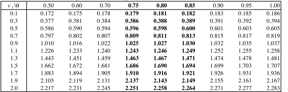
Then, appropriate values ofv2 are calculated with equation (4) for given
values of v1, ", and !, and the results are reported in tables 4 and 5 for the
UK and USA markets, respectively. The Newton-Raphson algorithm is used on equation (4) with the assumption of W0 = 1 to calculate v2. Since the
investment proportions in equity in the UK and USA are di!erent, we use di!erent values of " for the UK and US markets; for the UK market, we use
0.5"""1 and for the US market we use0.3"" "1.
The first panels of tables 4 and 5 shows the case of ! = 2.25 which is used in most studies. In this case, we have v2!v1 >0 for all given values.
However, we find evidence that the representative agents on both side of the atlantic are risk averse for gains and losses. That is, v2 >1 andv1 <1 can
be obtained only when v1 is very close to one, since the di!erence between
v1 andv2 is not large. In most cases,0< v2!v1 <0.3. In particular, for the
representative UK investor (" = 0.83) who is risk averse for gain (v1 < 1),
the di!erence between v2 and v1 is less than 0.1, and a similar pattern is
found in the USA market. As explained above, these results do di!er from many other multi-period studies which simply use v1 = v2. However, to be
more precise, we need v2 to be larger thanv1.
As explained in table 3, for a given value of v1, the values of v2 increase
as ! increases; see panels B and C in tables 4 and 5. Interestingly, when
! = 1.5, and for some ranges of v1, the values of v2 are less than those of
v1. See panel B of tables 4 and 5. Since we expect v2 > v1, these results
are unacceptable and suggest that the arbitrary value ! = 1.5 is too small. Thus, our results indirectly indicate that ! = 2.25 which is widely used in empirical finance is in the admissible range. In fact, all three parameters in the LA utility function, v1, v2 and !, are closely connected to each other
and a value of one parameter may not be justified independently of other parameters. Unfortunately, our study cannot reveal a unique set of v1 and
v2, but it does tell us what are appropriate sets of v1 and v2. If we assume
v1 = 0.88 as in Kahnemann and Tversky (1979) and others, thenv2 should
be around one.
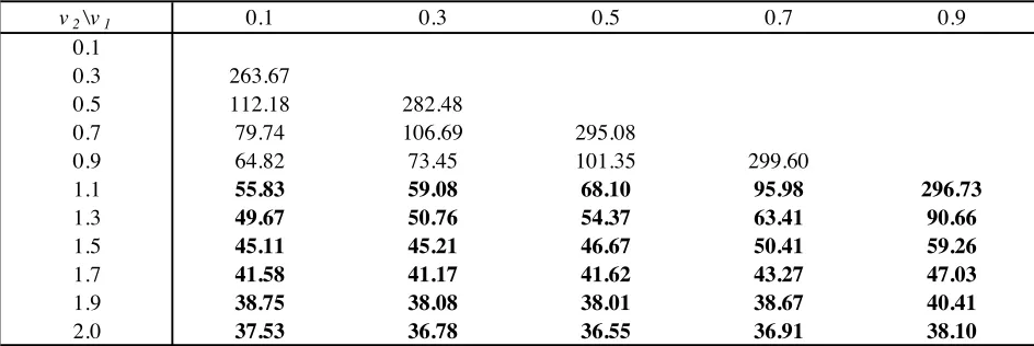
Finally we use normal distribution to find out the relationship between
market except the normal distribution.3 Using the estimates of mean and standard deviation in table 1, we numerically calculated the values of " for given values ofv1,v2, and!and reported the results in table 6. We could not
obtain the values of " when v2 !v1 " 0 and v1 > 1 because of convergence
errors. Table 6 suggests that the values of " for the admissable ranges of
v2 !v1 > 0 are extremely large and unrealistic; i.e., at least 2600% when
! = 2.25! As explained in table 3, when ! = 1.5 or ! = 3, the equity investment proportion increases or decreases.
We next calculate appropriate values of v2 with equation (4) for given
values of v1, ", and! under the normality assumption. The results in table
7 also confirm that v2 and v2 are close. However, when tables 4 and 7 are
compared, the values of v2 obtained with normality are always less than
those with the KST distribution. As a result of this, when ! = 1.5, we have v1 > v2 which contradicts proposition 2. In addition, when ! = 2.25
and v1 > 1, we also have v1 > v2. Only when ! is large enough, i.e., large
panalty for losses, proposition 2 is satistied. This is because normality does not capture extreme events adequately and thus we need large value of ! to compensate. For any distribution such as the KST distribution which can explain fat-tails of returns, we do not need large !. Therefore, the results in tables 6 and 7 indicate that we should be more careful when we use normality for the LA utility function.
4
Conclusions
In this study we used the LA utility function to explain the asset allocation. We first developed a few conditions that the LA utility function should sat-isfy. We showed that under fairly general conditions, the LA utility function becomes CARA class of utility functions. This is an interesting result in the sense that bahavoural finance such as prospect theory can be explained with the expected utility theory. In addition, we also proved that the curvature for the losses (v2) should be larger than that for the gains (v1). This result
is important because so far most studies such as Kahnemann and Tversky (1979), Benartzi and Thaler (1995), and Ang, Bekeart, and Liu (2000) used the same value for v1 andv2.
These results are supported by the empirical tests. In this study, we used a fairly general asymmetric distribution, Knight, Satchell and Tran (1995) distribution for the UK and US markets. We found thatv1andv2are close to
each other and v2!v1 is positive for the ranges of parameter values used by
other previous studies. For comparison purpose, however, when we assume
References
Ang, A., G. Bekeart, and J. Liu, 2000, ”Why Stocks May Disappoint,” Na-tional Bureau of Economic Research Working Paper Series 7783.
Arrow, K. J., 1971, Essays in the Theory of Risk-bearing, North-Hoolland, Amsterdam.
Barbersis, N., M. Huang, and T. Santos, 2001, ”Prospect Theory and Asset Prices,” Quarterly Journal of Economics 116(1), 1-53.
Berkelaar, A. and R. Kouwenberg, 2000, ”From Boom til Bust: How Loss Aversion A!ects Asset Prices,” Econometric Institute Report EI2000-21/A, Erasmus University Rotterdam, Netherlands.
Berkelaar, A. and R. Kouwenberg, 2000, ”Optimal Portfolio Choice Under Loss Aversion,” Econometric Institute Report EI2000-08/A, Erasmus Uni-versity Rotterdam, Netherlands.
Benartzi, S. and R. H. Thaler, 1995, ”Myopic Loss Aversion and the Equity Premium Puzzle”, Quarterly Journal of Economics 110(1), 73-92.
Bond, S., 2001, ”The Development of Dynamic Models of Semi-variance,” PhD Dissertation, Faculty of Economics and Politics, Cambridge University. Campbell, J. and L. Viceira, 1999, ”Comsumption and Portfolio Decisions When Expected Returns are Time-varying”,Quarterly Journal of Economics 114, 433-495.
Damant, D. C., S. Hwang, and S. E. Satchell, 2000, ”Exponential Risk Mea-sure with Application to UK Asset Allocation,” Applied Mathematical Fi-nance 7, 127-152.
De Bondt, W. F. M. and R. H. Thaler, 1985, ”Does the Stock Market Over-react?”, Journal of Finance 40, 793-805.
Fishburn, P. C. and G. A. Kochenberger, 1979, ”Concepts, Theory, Tech-niques; Two-piece Von Newmann-Morgenstern Utility Functions”, Decision Sciences 10, 503-518.
Friend, I. and M. E. Blume, 1975, ”The Demand for Risky Assets,”American
Economic Review 65, 900-922.
Gul, F., 1991, ”A Theory of Disappointment Aversion”,Econometrica 59(3), 667-686.
Hamilton, J. D., 1989, ”A New Approach to the Economics and Analysis of Nonstationary Time Series and the Business Cycle,” Econometrica 57, 357-84.
Kahnemann, D. and A. Tversky, 1979, ”Prospect Theory: An Analysis of Decision Under Risk”, Econometrica 47, 263-291.
Kehoe, P. J., 1983, ”Dynamics of the Current Account: Theorectical and Empirical Analysis,” Working paper, Harvard University.
Knight, J. L., S. E. Satchell, and K. C. Tran, 1995, ”Statistical Modelling of Asymmetric Risk in Asset Returns,” Applied Mathematical Finance 2, 155-172.
Kydland, F. E. and E. C. Prescott, 1982, ”Time to Build and Aggregate Fluctuations,” Econometrica 50, 1345-1370.
Mehra, R. and E. C. Prescott, 1985, ”The Equity Premium: A Puzzle”,
Journal of Monetary Economics 15, 145-161.
Pedersen, C. and S. E. Satchell, 2001, ”?????”, ???
Table 1 Properties of FT All-share and S&P500 Index Returns
A. FT All-share Index Returns
Mean Standard Deviation Skewness Excess Kurtosis Jarque-Bera Statistic
Entire Sample Period FT All-share Index Returns 1.4778 4.7757 -1.0937 * 4.6576 * 280.23 *
(January 1980 - 3 Month Treasury Bill Returns 0.7706 0.2668 0.3514 * -1.0206 * 16.25 *
February 2001) Excess Returns 0.7071 4.7782 -1.1444 * 4.6906 * 288.30 *
Sub-period 1 FT All-share Index Returns 1.9545 5.4103 -1.6334 * 6.3792 * 256.83 *
(January 1980 - 3 Month Treasury Bill Returns 0.9449 0.1858 0.4593 * -0.7005 6.67 *
December 1989) Excess Returns 1.0096 5.4156 -1.6298 * 6.2323 * 247.33 *
Sub-period 2 FT All-share Index Returns 1.0509 4.0996 -0.1943 0.2596 1.22
(January 1990 - 3 Month Treasury Bill Returns 0.6146 0.2293 1.4753 * 1.0741 * 55.05 *
February 2001) Excess Returns 0.4363 4.1271 -0.2576 0.1899 1.68
Lags Entire Sample Period Sub-period 1 Sub-period 2
(January 1980 - (January 1980 - (January 1990
-Autocorrelations February 2001) December 1989) February 2001)
of Excess Returns 1 -0.0267 -0.0805 0.0584
2 -0.1133 -0.1010 -0.1219
3 -0.1016 -0.0860 -0.1444
4 0.0240 0.0186 0.0125
5 -0.0032 -0.0448 0.0316
6 -0.1109 -0.1188 -0.1548
B. S&P500 Index Returns
Mean Standard Deviation Skewness Excess Kurtosis Jarque-Bera Statistic
Entire Sample Period S&P500 Index Returns 1.3398 4.4019 -0.6739 * 2.9716 * 112.68 *
(January 1980 - 3 Month Treasury Bill Returns 0.5620 0.2349 1.1985 * 1.1447 * 74.68 *
February 2001) Excess Returns 0.7777 4.4230 -0.6741 * 2.8098 * 102.79 *
Sub-period 1 S&P500 Index Log-returns 1.4721 4.7445 -0.7913 * 4.0931 * 96.29 *
(January 1980 - 3 Month Treasury Bill Returns 0.7307 0.2280 0.8750 * -0.1112 15.38 *
December 1989) Excess Returns 0.7414 4.7837 -0.7458 * 3.7082 * 79.88 *
Sub-period 2 S&P500 Index Log-returns 1.2213 4.0851 -0.5389 * 1.1294 * 13.61 *
(January 1990 - 3 Month Treasury Bill Returns 0.4110 0.0992 0.2801 0.2538 2.11
February 2001) Excess Returns 0.8103 4.0910 -0.5582 * 1.1411 * 14.23 *
Lags Entire Sample Period Sub-period 1 Sub-period 2
(January 1980 - (January 1980 - (January 1990
-Autocorrelations February 2001) December 1989) February 2001)
of Excess Returns 1 -0.0290 0.0563 -0.1349
2 -0.0293 -0.0791 0.0349
3 -0.0365 -0.0672 -0.0141
4 -0.0733 -0.0311 -0.1355
5 0.1098 0.1571 0.0542
6 -0.0329 0.0361 -0.1005
Table 2 Estimates of KST Parameters for the UK Returns
A. FT All-share Index Excess Returns
Entire Sample Period Sub-period 1 Sub-period 2
(January 1980 - February 2001) (January 1980 - December 1989) (January 1990 - February 2001)
!1 42.256 (5.136) 48.420 (8.162) 40.403 (7.061)
"1 1.467 (0.150) 1.870 (0.275) 1.244 (0.178)
!2 27.751 (4.484) 23.495 (5.818) 33.002 (7.008)
"2 1.066 (0.136) 1.054 (0.206) 1.109 (0.188)
Probability of Positive Excess Return (p) 0.622 0.658 0.590
Maximum Likelihood Value 427.896 194.958 238.115
B. S&P500 Index Excess Returns
Entire Sample Period Sub-period 1 Sub-period 2
(January 1980 - February 2001) (January 1980 - December 1989) (January 1990 - February 2001)
!1 40.296 (4.968) 37.426 (6.868) 43.439 (7.225)
"1 1.395 (0.144) 1.394 (0.213) 1.410 (0.196)
!2 34.249 (5.384) 29.747 (6.698) 40.644 (8.917)
"2 1.173 (0.149) 1.022 (0.180) 1.388 (0.254)
Probability of Positive Excess Return (p) 0.610 0.583 0.634
Maximum Likelihood Value 437.035 199.495 239.119
Table 3 Proportion in Equity for Given Sets of v1 and v2 for the Entire Sample Period
for the UK Market with the KST Distribution
A. The Proportion in Equity (!) for the Entire Sample Period (January 1980-February 2001) with l=2.25
v2\v1 0.2 0.4 0.6 0.8 1.0 1.2 1.4 1.6 1.8 2.0 3.0 5.0 10.0 20.0
0.2 154.03 66.04 47.78 39.53 34.58 31.16 28.58 26.53 24.84 19.26 13.73 8.25 4.69
0.4 6.48 142.43 59.68 43.04 35.65 31.27 28.26 25.99 24.20 18.59 13.26 8.03 4.60
0.6 12.79 5.01 141.21 56.23 40.01 32.99 28.90 26.12 24.06 18.12 12.88 7.84 4.52
0.8 15.19 10.36 3.79 147.60 54.69 38.11 31.15 27.18 24.53 17.85 12.57 7.67 4.44
1.0 15.98 12.59 8.40 2.82 160.78 54.54 36.99 29.89 25.92 17.78 12.33 7.52 4.38
1.2 16.07 13.46 10.50 6.81 2.07 181.06 55.51 36.48 29.05 17.93 12.14 7.39 4.32
1.4 15.83 13.70 11.43 8.80 5.52 1.50 209.54 57.46 36.45 18.38 12.02 7.27 4.26
1.6 15.44 13.63 11.78 9.76 7.40 4.47 1.08 248.09 60.33 19.25 11.94 7.17 4.21
1.8 14.99 13.41 11.84 10.20 8.38 6.24 3.62 0.77 299.46 20.78 11.93 7.07 4.16
2.0 14.51 13.11 11.75 10.36 8.88 7.22 5.28 2.94 0.55 23.53 11.98 6.99 4.11
3.0 12.26 11.37 10.54 9.74 8.96 8.19 7.39 6.56 5.67 4.69 13.79 6.74 3.93
5.0 9.17 8.68 8.23 7.80 7.40 7.02 6.65 6.29 5.94 5.60 3.79 7.01 3.70
10.0 5.61 5.41 5.22 5.04 4.88 4.72 4.58 4.44 4.30 4.17 3.58 2.52 3.81
20.0 3.17 3.10 3.03 2.96 2.90 2.84 2.78 2.73 2.68 2.63 2.40 2.03 1.28
B. The Proportion in Equity (!) for the Entire Sample Period (January 1980-February 2001) with l=1.5
v2\v1 0.2 0.4 0.6 0.8 1.0 1.2 1.4 1.6 1.8 2.0 3.0 5.0 10.0 20.0
0.2 20.28 23.96 24.31 23.81 23.06 22.23 21.39 20.59 19.83 16.67 12.62 7.92 4.59
0.4 49.21 18.76 21.66 21.90 21.48 20.85 20.15 19.46 18.78 15.90 12.14 7.70 4.50
0.6 35.23 38.08 18.60 20.40 20.36 19.88 19.27 18.63 18.01 15.31 11.75 7.51 4.42
0.8 29.85 28.56 28.81 19.44 19.84 19.39 18.77 18.12 17.49 14.84 11.42 7.34 4.35
1.0 26.52 24.76 23.15 21.43 21.17 19.79 18.82 18.00 17.28 14.51 11.14 7.19 4.29
1.2 24.10 22.34 20.65 18.76 15.72 23.84 20.15 18.56 17.50 14.31 10.91 7.05 4.22
1.4 22.19 20.55 18.97 17.30 15.21 11.41 27.59 20.85 18.55 14.27 10.74 6.93 4.17
1.6 20.63 19.12 17.67 16.20 14.55 12.32 8.21 32.67 21.89 14.41 10.60 6.83 4.12
1.8 19.31 17.92 16.60 15.30 13.91 12.27 9.99 5.86 39.43 14.82 10.51 6.73 4.07
2.0 18.17 16.89 15.69 14.52 13.31 11.99 10.37 8.10 4.16 15.68 10.47 6.65 4.02
3.0 14.17 13.29 12.48 11.71 10.98 10.25 9.52 8.77 7.95 7.03 11.26 6.36 3.83
5.0 9.98 9.48 9.02 8.59 8.19 7.81 7.45 7.09 6.75 6.41 4.64 6.46 3.60
10.0 5.84 5.64 5.45 5.27 5.10 4.95 4.80 4.65 4.52 4.39 3.79 2.74 3.66
20.0 3.24 3.16 3.09 3.02 2.96 2.90 2.84 2.79 2.74 2.69 2.46 2.08 1.33
C. The Proportion in Equity (!) for the Entire Sample Period (January 1980-February 2001) with l=3
v2\v1 0.2 0.4 0.6 0.8 1.0 1.2 1.4 1.6 1.8 2.0 3.0 5.0 10.0 20.0
0.2 649.07 135.56 77.17 56.64 46.11 39.60 35.10 31.76 29.15 21.35 14.58 8.50 4.75
0.4 1.54 600.22 122.52 69.52 51.08 41.69 35.91 31.92 28.97 20.76 14.12 8.28 4.67
0.6 6.23 1.19 595.07 115.42 64.63 47.27 38.54 33.20 29.54 20.43 13.75 8.08 4.58
0.8 9.40 5.05 0.90 621.96 112.26 61.55 44.63 36.24 31.17 20.34 13.46 7.91 4.51
1.0 11.15 7.80 4.09 0.67 677.52 111.96 59.75 42.82 34.56 20.53 13.25 7.76 4.45
1.2 12.05 9.39 6.50 3.32 0.49 762.98 113.96 58.93 41.63 21.04 13.10 7.63 4.38
1.4 12.46 10.28 7.98 5.45 2.69 0.36 882.99 117.96 58.88 22.00 13.01 7.52 4.33
1.6 12.57 10.73 8.84 6.81 4.58 2.18 0.26 1045.43 123.84 23.64 13.00 7.42 4.27
1.8 12.52 10.92 9.32 7.65 5.85 3.86 1.77 0.18 1261.91 26.41 13.05 7.33 4.23
2.0 12.36 10.95 9.56 8.15 6.66 5.04 3.27 1.43 0.13 31.37 13.19 7.25 4.18
3.0 11.06 10.18 9.35 8.55 7.76 6.98 6.18 5.34 4.46 3.52 15.92 7.02 3.99
5.0 8.64 8.16 7.71 7.29 6.89 6.51 6.14 5.78 5.43 5.08 3.28 7.42 3.77
10.0 5.44 5.25 5.06 4.89 4.73 4.57 4.43 4.29 4.15 4.02 3.43 2.38 3.92
20.0 3.13 3.05 2.98 2.92 2.86 2.80 2.74 2.69 2.63 2.58 2.36 1.99 1.24
Table 4 The Values of v2 for Given Sets of v1 and Investment Proportion in Equity for the
Entire Sample Period (January 1980-February 2001) in the UK Market with the KST Distribution
A. The Estimated Values of v2 for Given Sets of v1 and ! with l=2.25
v1\# 0.50 0.60 0.70 0.75 0.80 0.85 0.90 0.95 1.00
0.1 0.172 0.175 0.178 0.179 0.181 0.182 0.183 0.185 0.186
0.3 0.377 0.381 0.384 0.386 0.388 0.389 0.391 0.392 0.394
0.5 0.586 0.590 0.594 0.596 0.598 0.600 0.601 0.603 0.605
0.7 0.797 0.802 0.807 0.809 0.811 0.813 0.815 0.817 0.819
0.9 1.010 1.016 1.022 1.025 1.027 1.030 1.032 1.035 1.037
1.1 1.226 1.233 1.240 1.243 1.246 1.249 1.252 1.255 1.258
1.3 1.443 1.451 1.459 1.463 1.467 1.471 1.474 1.478 1.481
1.5 1.662 1.672 1.681 1.686 1.690 1.694 1.699 1.703 1.707
1.7 1.883 1.894 1.905 1.910 1.916 1.921 1.926 1.931 1.936
1.9 2.105 2.119 2.131 2.137 2.143 2.149 2.155 2.161 2.167
2.0 2.217 2.231 2.245 2.251 2.258 2.264 2.271 2.277 2.283
B. The Estimated Values of v2 for Given Sets of v1 and ! with l=1.5
v1\# 0.50 0.60 0.70 0.75 0.80 0.85 0.90 0.95 1.00
0.1 0.078 0.077 0.076 0.076 0.075 0.075 0.075 0.074 0.074
0.3 0.278 0.277 0.276 0.276 0.275 0.275 0.275 0.274 0.274
0.5 0.482 0.481 0.480 0.480 0.479 0.479 0.478 0.478 0.478
0.7 0.688 0.688 0.687 0.687 0.686 0.686 0.686 0.686 0.685
0.9 0.897 0.897 0.897 0.897 0.897 0.897 0.897 0.896 0.896
1.1 1.108 1.109 1.109 1.109 1.110 1.110 1.110 1.110 1.110
1.3 1.322 1.323 1.324 1.325 1.325 1.326 1.326 1.327 1.327
1.5 1.537 1.539 1.541 1.542 1.543 1.544 1.545 1.546 1.547
1.7 1.754 1.757 1.760 1.762 1.763 1.765 1.766 1.768 1.769
1.9 1.973 1.977 1.982 1.984 1.986 1.988 1.990 1.992 1.994
2.0 2.083 2.088 2.093 2.095 2.098 2.100 2.102 2.105 2.107
C. The Estimated Values of v2 for Given Sets of v1 and ! with l=3
v1\# 0.50 0.60 0.70 0.75 0.80 0.85 0.90 0.95 1.00
0.1 0.240 0.247 0.252 0.255 0.258 0.261 0.263 0.266 0.268
0.3 0.449 0.457 0.463 0.466 0.469 0.472 0.475 0.478 0.481
0.5 0.661 0.669 0.677 0.681 0.684 0.688 0.691 0.694 0.698
0.7 0.876 0.885 0.894 0.898 0.902 0.906 0.910 0.913 0.917
0.9 1.092 1.103 1.113 1.117 1.122 1.127 1.131 1.135 1.140
1.1 1.310 1.322 1.334 1.339 1.345 1.350 1.355 1.360 1.365
1.3 1.531 1.544 1.557 1.563 1.569 1.576 1.581 1.587 1.593
1.5 1.752 1.768 1.783 1.790 1.797 1.804 1.810 1.817 1.824
1.7 1.976 1.993 2.010 2.018 2.026 2.034 2.041 2.049 2.057
1.9 2.201 2.221 2.239 2.248 2.257 2.266 2.275 2.284 2.292
2.0 2.314 2.335 2.355 2.364 2.374 2.383 2.393 2.402 2.411
Notes: The values of v2 are calculated with the estimates of the KST distribution for the entire sample period;
Table 5 The Values of v2 for Given Sets of v1 and Investment Proportion in Equity for the
Entire Sample Period (January 1980-February 2001) in the US Market with the KST Distribution
A. The Estimated Values of v2 for Given Sets of v1 and ! with l=2.25
v1\# 0.30 0.40 0.45 0.50 0.55 0.60 0.65 0.70 0.80 0.9 1
0.1 0.172 0.177 0.179 0.181 0.183 0.184 0.186 0.188 0.191 0.194 0.196 0.3 0.373 0.378 0.380 0.383 0.384 0.386 0.388 0.390 0.393 0.396 0.399 0.5 0.576 0.581 0.583 0.585 0.587 0.589 0.591 0.593 0.597 0.600 0.603 0.7 0.778 0.784 0.786 0.789 0.791 0.793 0.795 0.797 0.801 0.805 0.809 0.9 0.982 0.988 0.991 0.993 0.996 0.998 1.000 1.003 1.007 1.011 1.015 1.1 1.186 1.193 1.196 1.199 1.201 1.204 1.206 1.209 1.213 1.218 1.222 1.3 1.391 1.398 1.401 1.404 1.407 1.410 1.413 1.416 1.421 1.426 1.430 1.5 1.596 1.604 1.608 1.611 1.614 1.617 1.620 1.623 1.629 1.634 1.640 1.7 1.802 1.811 1.814 1.818 1.822 1.825 1.828 1.832 1.838 1.844 1.850 1.9 2.009 2.018 2.022 2.026 2.030 2.033 2.037 2.040 2.047 2.054 2.060 2.0 2.112 2.121 2.126 2.130 2.134 2.138 2.141 2.145 2.152 2.159 2.166
B. The Estimated Values of v2 for Given Sets of v1 and ! with l=1.5
v1\# 0.30 0.40 0.45 0.50 0.55 0.60 0.65 0.70 0.80 0.9 1
0.1 0.090 0.089 0.089 0.088 0.088 0.088 0.088 0.088 0.087 0.087 0.086 0.3 0.287 0.286 0.286 0.286 0.285 0.285 0.285 0.284 0.284 0.283 0.283 0.5 0.486 0.485 0.485 0.484 0.484 0.483 0.483 0.483 0.482 0.481 0.481 0.7 0.686 0.685 0.684 0.684 0.684 0.683 0.683 0.682 0.682 0.681 0.680 0.9 0.887 0.886 0.885 0.885 0.884 0.884 0.884 0.883 0.883 0.882 0.881 1.1 1.088 1.087 1.087 1.087 1.086 1.086 1.085 1.085 1.085 1.084 1.083 1.3 1.290 1.290 1.289 1.289 1.289 1.289 1.288 1.288 1.287 1.287 1.286 1.5 1.493 1.493 1.493 1.492 1.492 1.492 1.492 1.492 1.491 1.491 1.491 1.7 1.697 1.697 1.697 1.696 1.696 1.696 1.696 1.696 1.696 1.696 1.696 1.9 1.901 1.901 1.901 1.901 1.901 1.901 1.901 1.901 1.901 1.901 1.901 2.0 2.003 2.003 2.004 2.004 2.004 2.004 2.004 2.004 2.004 2.004 2.005
C. The Estimated Values of v2 for Given Sets of v1 and ! with l=3
v1\# 0.30 0.40 0.45 0.50 0.55 0.60 0.65 0.70 0.80 0.9 1
0.1 0.232 0.240 0.244 0.248 0.251 0.254 0.257 0.260 0.266 0.271 0.277 0.3 0.436 0.445 0.449 0.453 0.456 0.460 0.463 0.466 0.472 0.478 0.484 0.5 0.640 0.650 0.654 0.658 0.662 0.666 0.669 0.673 0.680 0.686 0.692 0.7 0.845 0.855 0.860 0.864 0.869 0.873 0.877 0.881 0.888 0.895 0.902 0.9 1.051 1.062 1.067 1.072 1.076 1.081 1.085 1.089 1.097 1.104 1.112 1.1 1.257 1.269 1.274 1.279 1.284 1.289 1.294 1.298 1.307 1.315 1.323 1.3 1.463 1.476 1.482 1.487 1.493 1.498 1.503 1.508 1.517 1.526 1.535 1.5 1.670 1.684 1.690 1.696 1.702 1.708 1.713 1.718 1.728 1.738 1.748 1.7 1.878 1.892 1.899 1.906 1.912 1.918 1.923 1.929 1.940 1.951 1.961 1.9 2.086 2.101 2.108 2.115 2.122 2.128 2.135 2.141 2.153 2.164 2.175 2.0 2.190 2.206 2.213 2.220 2.227 2.234 2.240 2.247 2.259 2.271 2.283 Notes: The values of v2 are calculated with the estimates of the KST distribution for the entire sample period;
Table 6 Proportion in Equity for Given Sets of v1 and v2 for the Entire Sample Period
for the UK Market with the Normal Distribution
A. The Proportion in Equity (!) for the Entire Sample Period (January 1980-February 2001) with l=2.25
v2\v1 0.1 0.3 0.5 0.7 0.9
0.1
0.3 34.72
0.5 40.71 37.20
0.7 40.57 38.72 38.86
0.9 39.05 37.37 36.78 39.46
1.1 37.22 35.59 34.64 34.82 39.09
1.3 35.43 33.84 32.75 32.26 32.85
1.5 33.77 32.25 31.11 30.36 30.15
1.7 32.27 30.82 29.69 28.85 28.31
1.9 30.93 29.56 28.45 27.58 26.94
2.0 30.32 28.98 27.89 27.02 26.36
B. The Proportion in Equity (!) for the Entire Sample Period (January 1980-February 2001) with l=1.5
v2\v1 0.1 0.3 0.5 0.7 0.9
0.1
0.3 263.67
0.5 112.18 282.48
0.7 79.74 106.69 295.08
0.9 64.82 73.45 101.35 299.60
1.1 55.83 59.08 68.10 95.98 296.73
1.3 49.67 50.76 54.37 63.41 90.66
1.5 45.11 45.21 46.67 50.41 59.26
1.7 41.58 41.17 41.62 43.27 47.03
1.9 38.75 38.08 38.01 38.67 40.41
2.0 37.53 36.78 36.55 36.91 38.10
C. The Proportion in Equity (!) for the Entire Sample Period (January 1980-February 2001) with l=3
v2\v1 0.1 0.3 0.5 0.7 0.9
0.1
0.3 8.24
0.5 19.83 8.83
0.7 25.12 18.86 9.22
0.9 27.25 23.14 17.92 9.37
1.1 27.92 24.84 21.45 16.97 9.28
1.3 27.88 25.38 22.86 19.97 16.03
1.5 27.50 25.37 23.33 21.19 18.66
1.7 26.96 25.10 23.36 21.64 19.77
1.9 26.36 24.69 23.17 21.70 20.21
2.0 26.06 24.47 23.03 21.66 20.29
Table 7 The Values of v2 for Given Sets of v1 and Investment Proportion in Equity for the
Entire Sample Period (January 1980-February 2001) in the UK Market with the Normal Distribution
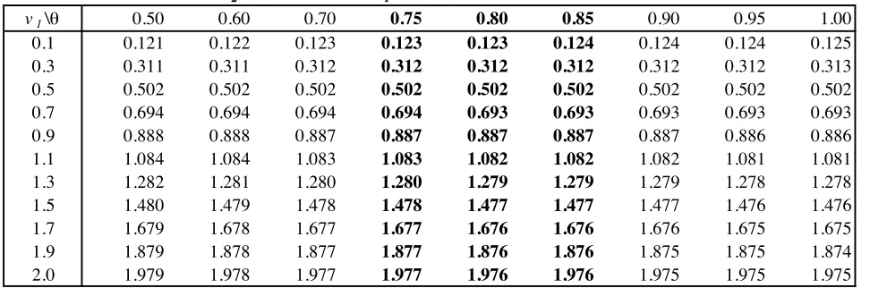
A. The Estimated Values of v2 for Given Sets of v1 and ! with l=2.25
v1\# 0.50 0.60 0.70 0.75 0.80 0.85 0.90 0.95 1.00
0.1 0.121 0.122 0.123 0.123 0.123 0.124 0.124 0.124 0.125
0.3 0.311 0.311 0.312 0.312 0.312 0.312 0.312 0.312 0.313
0.5 0.502 0.502 0.502 0.502 0.502 0.502 0.502 0.502 0.502
0.7 0.694 0.694 0.694 0.694 0.693 0.693 0.693 0.693 0.693
0.9 0.888 0.888 0.887 0.887 0.887 0.887 0.887 0.886 0.886
1.1 1.084 1.084 1.083 1.083 1.082 1.082 1.082 1.081 1.081
1.3 1.282 1.281 1.280 1.280 1.279 1.279 1.279 1.278 1.278
1.5 1.480 1.479 1.478 1.478 1.477 1.477 1.477 1.476 1.476
1.7 1.679 1.678 1.677 1.677 1.676 1.676 1.676 1.675 1.675
1.9 1.879 1.878 1.877 1.877 1.876 1.876 1.875 1.875 1.874
2.0 1.979 1.978 1.977 1.977 1.976 1.976 1.975 1.975 1.975
B. The Estimated Values of v2 for Given Sets of v1 and ! with l=1.5
v1\# 0.50 0.60 0.70 0.75 0.80 0.85 0.90 0.95 1.00
0.1 0.038 0.036 0.033 0.032 0.031 0.030 0.029 0.029 0.028
0.3 0.224 0.221 0.218 0.217 0.216 0.215 0.213 0.212 0.211
0.5 0.412 0.408 0.405 0.403 0.401 0.400 0.399 0.397 0.396
0.7 0.601 0.597 0.593 0.591 0.589 0.587 0.586 0.584 0.582
0.9 0.792 0.787 0.783 0.781 0.779 0.777 0.775 0.773 0.771
1.1 0.985 0.980 0.975 0.973 0.971 0.969 0.966 0.964 0.962
1.3 1.180 1.175 1.169 1.167 1.164 1.162 1.160 1.158 1.155
1.5 1.376 1.370 1.365 1.362 1.360 1.357 1.355 1.352 1.350
1.7 1.574 1.568 1.562 1.559 1.556 1.554 1.551 1.549 1.546
1.9 1.772 1.765 1.759 1.757 1.754 1.751 1.748 1.746 1.743
2.0 1.871 1.865 1.859 1.856 1.853 1.850 1.847 1.845 1.842
C. The Estimated Values of v2 for Given Sets of v1 and ! with l=3
v1\# 0.50 0.60 0.70 0.75 0.80 0.85 0.90 0.95 1.00
0.1 0.181 0.184 0.187 0.189 0.190 0.191 0.192 0.194 0.195
0.3 0.373 0.376 0.379 0.380 0.381 0.383 0.384 0.385 0.386
0.5 0.566 0.569 0.572 0.573 0.574 0.575 0.577 0.578 0.579
0.7 0.761 0.764 0.766 0.768 0.769 0.770 0.771 0.772 0.773
0.9 0.958 0.960 0.963 0.964 0.965 0.966 0.967 0.968 0.969
1.1 1.155 1.158 1.160 1.162 1.163 1.164 1.165 1.166 1.167
1.3 1.354 1.357 1.359 1.361 1.362 1.363 1.364 1.365 1.366
1.5 1.554 1.557 1.559 1.561 1.562 1.563 1.564 1.565 1.566
1.7 1.755 1.758 1.760 1.761 1.763 1.764 1.765 1.766 1.767
1.9 1.956 1.959 1.961 1.963 1.964 1.965 1.966 1.967 1.969
2.0 2.056 2.059 2.062 2.063 2.065 2.066 2.067 2.068 2.069
!
!"#$%&'()*)+#,(,+#%+,(
(
List of other working papers:
2001
1. Soosung Hwang and Steve Satchell , GARCH Model with Cross-sectional Volatility; GARCHX
Models, WP01-16
2. Soosung Hwang and Steve Satchell, Tracking Error: Ex-Ante versus Ex-Post Measures,
WP01-15
3. Soosung Hwang and Steve Satchell, The Asset Allocation Decision in a Loss Aversion World,
WP01-14
4. Soosung Hwang and Mark Salmon, An Analysis of Performance Measures Using Copulae,
WP01-13
5. Soosung Hwang and Mark Salmon, A New Measure of Herding and Empirical Evidence,
WP01-12
6. Richard Lewin and Steve Satchell, The Derivation of New Model of Equity Duration,
WP01-11
7. Massimiliano Marcellino and Mark Salmon, Robust Decision Theory and the Lucas Critique,
WP01-10
8. Jerry Coakley, Ana-Maria Fuertes and Maria-Teresa Perez, Numerical Issues in Threshold Autoregressive Modelling of Time Series, WP01-09
9. Jerry Coakley, Ana-Maria Fuertes and Ron Smith, Small Sample Properties of Panel
Time-series Estimators with I(1) Errors, WP01-08
10. Jerry Coakley and Ana-Maria Fuertes, The Felsdtein-Horioka Puzzle is Not as Bad as You Think, WP01-07
11. Jerry Coakley and Ana-Maria Fuertes, Rethinking the Forward Premium Puzzle in a
Non-linear Framework, WP01-06
12. George Christodoulakis, Co-Volatility and Correlation Clustering: A Multivariate Correlated ARCH Framework, WP01-05
13. Frank Critchley, Paul Marriott and Mark Salmon, On Preferred Point Geometry in Statistics, WP01-04
14. Eric Bouyé and Nicolas Gaussel and Mark Salmon, Investigating Dynamic Dependence Using
Copulae, WP01-03
15. Eric Bouyé, Multivariate Extremes at Work for Portfolio Risk Measurement, WP01-02 16. Erick Bouyé, Vado Durrleman, Ashkan Nikeghbali, Gael Riboulet and Thierry Roncalli,
Copulas: an Open Field for Risk Management, WP01-01
2000
1. Soosung Hwang and Steve Satchell , Valuing Information Using Utility Functions, WP00-06
2. Soosung Hwang, Properties of Cross-sectional Volatility, WP00-05
3. Soosung Hwang and Steve Satchell, Calculating the Miss-specification in Beta from Using a Proxy for the Market Portfolio, WP00-04
4. Laun Middleton and Stephen Satchell, Deriving the APT when the Number of Factors is
Unknown, WP00-03
5. George A. Christodoulakis and Steve Satchell, Evolving Systems of Financial Returns: Auto-Regressive Conditional Beta, WP00-02
6. Christian S. Pedersen and Stephen Satchell, Evaluating the Performance of Nearest Neighbour Algorithms when Forecasting US Industry Returns, WP00-01
1999
2. Soosung Hwang, John Knight and Stephen Satchell, Forecasting Volatility using LINEX Loss Functions, WP99-20
3. Soosung Hwang and Steve Satchell, Improved Testing for the Efficiency of Asset Pricing
Theories in Linear Factor Models, WP99-19
4. Soosung Hwang and Stephen Satchell, The Disappearance of Style in the US Equity Market,
WP99-18
5. Soosung Hwang and Stephen Satchell, Modelling Emerging Market Risk Premia Using Higher
Moments, WP99-17
6. Soosung Hwang and Stephen Satchell, Market Risk and the Concept of Fundamental
Volatility: Measuring Volatility Across Asset and Derivative Markets and Testing for the Impact of Derivatives Markets on Financial Markets, WP99-16
7. Soosung Hwang, The Effects of Systematic Sampling and Temporal Aggregation on Discrete
Time Long Memory Processes and their Finite Sample Properties, WP99-15
8. Ronald MacDonald and Ian Marsh, Currency Spillovers and Tri-Polarity: a Simultaneous
Model of the US Dollar, German Mark and Japanese Yen, WP99-14
9. Robert Hillman, Forecasting Inflation with a Non-linear Output Gap Model, WP99-13
10.Robert Hillman and Mark Salmon , From Market Micro-structure to Macro Fundamentals: is
there Predictability in the Dollar-Deutsche Mark Exchange Rate?, WP99-12
11.Renzo Avesani, Giampiero Gallo and Mark Salmon, On the Evolution of Credibility and
Flexible Exchange Rate Target Zones, WP99-11
12.Paul Marriott and Mark Salmon, An Introduction to Differential Geometry in Econometrics, WP99-10
13.Mark Dixon, Anthony Ledford and Paul Marriott, Finite Sample Inference for Extreme Value
Distributions, WP99-09
14.Ian Marsh and David Power, A Panel-Based Investigation into the Relationship Between
Stock Prices and Dividends, WP99-08
15.Ian Marsh, An Analysis of the Performance of European Foreign Exchange Forecasters,
WP99-07
16.Frank Critchley, Paul Marriott and Mark Salmon, An Elementary Account of Amari's Expected
Geometry, WP99-06
17.Demos Tambakis and Anne-Sophie Van Royen, Bootstrap Predictability of Daily Exchange
Rates in ARMA Models, WP99-05
18.Christopher Neely and Paul Weller, Technical Analysis and Central Bank Intervention,
WP99-04
19.Christopher Neely and Paul Weller, Predictability in International Asset Returns: A Re-examination, WP99-03
20.Christopher Neely and Paul Weller, Intraday Technical Trading in the Foreign Exchange Market, WP99-02
21.Anthony Hall, Soosung Hwang and Stephen Satchell, Using Bayesian Variable Selection
Methods to Choose Style Factors in Global Stock Return Models, WP99-01
1998
1. Soosung Hwang and Stephen Satchell, Implied Volatility Forecasting: A Compaison of
Different Procedures Including Fractionally Integrated Models with Applications to UK Equity Options, WP98-05
2. Roy Batchelor and David Peel, Rationality Testing under Asymmetric Loss, WP98-04
3. Roy Batchelor, Forecasting T-Bill Yields: Accuracy versus Profitability, WP98-03
4. Adam Kurpiel and Thierry Roncalli , Option Hedging with Stochastic Volatility, WP98-02
5. Adam Kurpiel and Thierry Roncalli, Hopscotch Methods for Two State Financial Models,